Maximum-Likelihood Estimation With a Contracting-Grid Search Algorithm

Abstract

A fast search algorithm capable of operating in multi-dimensional spaces is introduced. As a sample application, we demonstrate its utility in the 2D and 3D maximum-likelihood position-estimation problem that arises in the processing of PMT signals to derive interaction locations in compact gamma cameras. We demonstrate that the algorithm can be parallelized in pipelines, and thereby efficiently implemented in specialized hardware, such as field-programmable gate arrays (FPGAs). A 2D implementation of the algorithm is achieved in Cell/BE processors, resulting in processing speeds above one million events per second, which is a 20× increase in speed over a conventional desktop machine. Graphics processing units (GPUs) are used for a 3D application of the algorithm, resulting in processing speeds of nearly 250,000 events per second which is a 250× increase in speed over a conventional desktop machine. These implementations indicate the viability of the algorithm for use in real-time imaging applications.

I. Introduction

A variety of inference tasks—2D and 3D position estimation, energy estimation, fluence estimation, spectral distributions, etc.—occur in science and engineering fields where data must be inverted to derive parameters of a physical model. Maximum-likelihood methods offer an attractive approach to solving inverse problems when the statistics of the forward problem are at least approximately known. ML estimation methods possess several desirable properties [1], [2]. They include:

• efficient if an efficient estimator exists,

• asymptotically efficient,

• asymptotically unbiased,

• independent of prior information.

The maximum-likelihood method can generally be formulated as a search over a parameter space,

$$\widehat{\mathit{\theta }}=arg\underset{\theta }{max}\lambda (\mathit{\theta }\mid \mathit{g})=arg\underset{\theta }{max}\text{pr}(\mathit{g}\mid \mathit{\theta })$$ (1)

where θ is a vector of parameters, g is a vector of observations (data), λ is the likelihood, and θ̂ is a vector of estimated model parameters. In some instances, the maximum-likelihood estimate may be solved directly. For example, in the case of independent, normally-distributed noise, the maximum-likelihood method is equivalent to a least-squares solution. The general method can be summarized in the form of a question: given a set of observations g, what is the set of parameters θ that has the highest probability of generating the observed data?.

The need to search multidimensional spaces (each parameter to be estimated adds one dimension) for extrema represents a fundamental research problem. Many techniques have been developed to address this problem, including conjugate gradient methods [3] and a host of others [4]. We have developed a new algorithm that falls in the class of variable-mesh, derivative-free optimization (DFO) algorithms [5]–[7]. More specifically, within this class, the algorithm belongs to a group of contracting-grid search methods [8], [9], that generalizes to ML-estimation problems in N-dimensional spaces. Finally, while this work examines a particular ML-estimation problem, the algorithm would work equally well for other problems requiring optimization of a utility function, most notably maximum a priori (MAP) estimation.

II. Algorithm Description

The algorithm allows identification of a function maximum (or minimum) in a fixed number of iterations that depends on the desired precision. If the function does not have local maxima (or minima), the search algorithm’s computational efficiency increases dramatically. The algorithm will be described for a general N-dimensional problem and has been successfully implemented in a 7-D estimation problem [10]. The algorithm will be illustrated in detail for a specific 2D/3D application: (x, y)/(x, y, z) position estimation in a modular scintillation camera. Incidence rates of 25000 photons-per-second or less are typical of acquisitions for this applications, although this number may vary greatly depending on the sensitivity and geometry of the camera system.

This section will describe implementation of the algorithm to the searching of an N-dimensional space (i.e., an N × 1 vector of parameters θ). For each parameter θ_i, we describe its physically reasonable domain with M_i discrete samples such that the distance between any two adjacent samples is smaller than or equal to the desired precision of the estimate, i.e., |θ_i(m + 1) − θ_i(m)| ≤ δ_i.

1. For each θ_i in θ, pad the regions at the end of the physically reasonable parameter space of size M_i with regions of zero event likelihood of width ceil((P_i − 3)M_i/4P_i), where P_i is the initial number of regions used to cover the parameter space (i.e., the grid dimension).¹

2. Pre-compute all terms in the likelihood that depend only on calibration data or prior knowledge, and scale appropriately to permit use of integer arithmetic.

3. for i = 1 to (ceil(log₂(max(M_i)) −2)) where the function ceil rounds to the nearest, larger integer,

   1. Compute the function at the test locations. The number of test locations for the first iteration will be ${\prod }_{i=1}^N{P}_i$. As the iteration number increases, the algorithm will converge in some domains and the number of computations (i.e., test locations) will decrease. In practice, we have found that it’s advantageous to delay converging on parameters that will require fewer steps until that number of steps remains in the global search.

   2. Select the location that returns the highest/lowest likelihood. This location will serve as the center of the next region of interest.

   3. For each parameter space that has not yet converged, decrease the test location grid spacing by a factor of 2 (other contraction rates may be used, but a factor-2 rate is convenient as it corresponds to a 1-bit shift in hardware implementations).

4. Evaluate the function at the remaining locations where the remaining locations are those grid points surrounding the maximum likelihood location of the final iteration in Step 3, given a step size of 1 grid point.. The highest/lowest value of these remaining points represents the maximum/minimum of the function over the space of interest.

One nice feature of the algorithm is that the number of computations in a given iteration scale with the grid spacing dimension P_i and not with the parameter dimension M_i. Also, prior knowledge of the behavior of the likelihood function within the multi-dimensional parameter space may be easily incorporated to tailor the search for optimum efficiency. For example, a broad grid spacing may be used for slowly varying, smooth likelihood functions. For more textured likelihood functions perhaps even with local maxima/minima, a built-in error tolerance (achieved by allowing successive grids to overlap into regions of the previous grid) combined with a fine grid spacing enables successful use of the algorithm. Another desirable feature of the algorithm is that a final solution is achieved in a known number of iterations. This feature is attractive for hardware implementation. The ease of implementation of the algorithm and ability to extend to multiple dimensions makes it an attractive option for a variety of applications, including 2D and 3D position estimation for nuclear-medicine cameras, estimation of pulse amplitude and timing of the detection of scintillation pulses, and wavefront sensing.

III. Application to 2D Position Estimation

The algorithm was first developed for performing 2D position estimation in modular scintillation cameras [11], [12]. This section will provide some background about modular cameras and their corresponding data-acquisition architecture, a thorough description of the algorithm’s application to the position estimation problem, and comparison to other methods.

A. Modular Gamma Cameras

The basic components of an Anger camera include a scintillation crystal, light guide (or optical window), and array of PMTs. The modular camera used in this study employs a 117 mm square, 5 mm thick thallium-doped sodium iodide crystal. This crystal is separated from a 3 × 3 array of 38.1 mm diameter PMTs by a 8 mm light guide. A thin plate of aluminum shields the crystal, serving as an entrance window. A white near-Lambertian reflector, separates the aluminum entrance window from the front crystal face. The diffuse rear crystal face is coupled to the light guide using optical-grade room temperature vulcanization (RTV) silicone. Black absorbing epoxy is used to hermetically seal the scintillation crystal and optical window. Index-matching RTV couples the light guide to the PMTs, each of which is wrapped in a CO-NETIC shield. Each PMT contains 10 dynode stages and operates at a voltage bias of ~800 V. A schematic and photo of a modular gamma camera are shown in Fig. 1.

Fig. 1.

(a) A schematic of a modular scintillation camera. (b) A photograph of a modular scintillation camera.

The basic operation of a gamma camera begins with the interaction of a gamma ray within a scintillation crystal. This interaction produces a burst of visible-light photons which disperse through the light guide to be spread over the array of PMTs. The PMTs convert the photons to a number of primary electrons that are then amplified by the successive dynode stages until a final current pulse is collected and processed by front-end electronics. The processing includes the analog-to-digital (A/D) conversion of the electrical signals. Back-end buffers accumulate lists of events during acquisition. In our systems, this process serves to convert ensembles of incident gamma rays into lists of nine 12-bit digital numbers and is known as super list-mode data acquisition.

The list-mode data is used with carefully acquired calibration data to determine the location of each gamma ray’s point of incidence on the camera face in a process known as position estimation. By performing position estimation on a collection of gamma rays, and binning each gamma ray into its location on the camera face into a 2D histogram, a projection image is generated.

Performing the task of position estimation with maximum-likelihood methods requires knowledge of the probability of the data, given the parameters to estimate—namely, x and y position. For example, a probability function of the form Pr(V_j|x, y) where V_j is the K × 1 vector of PMT outputs for event j (assuming a camera with K PMTs) is required for the 2D estimation problem. The output signal at each PMT anode is proportional to the number of primary photoelectrons produced at the PMT photocathode. The generation of these primary photoelectrons approximately obeys Poisson statistics [1], and the signals in different PMTs are independent. Thus, the probability of generating a particular list-mode data vector from an event at a particular location may be written in terms of the mean signals in each PMT resulting from events at that location. This scaled Poisson model may be expressed as,

$$Pr(\mathit{o}\mid x,y)=\prod _{k=1}^9\frac{{({\overline{o}}_k(x,y))}^{o_k}}{o_k!}exp(-{\overline{o}}_k(x,y)),$$ (2)

where ō_k(x, y) is the mean PMT output (assuming zero-mean fluctuations around PMT gain) for the kth PMT at a given location on the camera face (x, y) and o_k is the PMT output of the kth PMT for the event in question. The term o is a 9-element vector composed of the o_k.

B. Maximum-Likelihood Position Estimation

The log-likelihood expression (found by taking the natural log of (2)) is given by

$$\lambda (\mathit{o}\mid x,y)=\sum _{k=1}^9[o_{k}ln{\overline{o}}_k(x,y)-{\overline{o}}_k(x,y)-ln(o_k!)].$$ (3)

The computationally intensive task in ML position estimation is finding the (x, y) that maximizes the log-likelihood λ(x, y). This ML estimation process must be repeated for every event acquired.

C. Mean Detector Response Function

Likelihoods based on Poisson statistics are characterized by a single parameter, the mean signal. Hence, measurement of the mean detector response function (MDRF) is the only calibration procedure necessary to employ ML position estimation [13]. The MDRF matrix contains the mean PMT outputs, represented by ō in (3), for a collection of points on the camera face. The process of collecting the MDRF involves stepping a collimated source in a uniform grid over the camera face. The grid locations will define the camera pixels in the projection images, although it is generally possible to collect a sparse grid and interpolate intermediate locations. A typical MDRF for a 3 × 3 PMT modular camera consists of a 79 × 79 grid covering the camera face in 1.5 mm steps. At each point on the grid, the nine PMT output means are generated by applying a filtering window to eliminate scattered events. A representative mean data set is illustrated in Fig. 2. Each of the 79 × 79 pixels in one of the nine images in Fig. 2 represents the mean response of a particular PMT to a collimated source at that location on the camera face. Post-process smoothing and interpolation procedures are also typically applied to MDRF data.

Fig. 2.

Example of a typical mean file generated by an MDRF. Each pixel of each of the nine images represents the response of a given PMT to a point source centered over that location on the camera face.

D. Application of Contracting-Grid Search

The log-likelihood function, given in (3), evaluated with a single event’s nine PMT values, will produce a likelihood map of dimension M × M, where M is the MDRF dimension (e.g. M = 79). An example likelihood map is shown in Fig. 3(a). The likelihood map representing the camera face has been padded with a border of zero event probability, allowing the search algorithm to be implemented without conditionals (i.e., “if” statements that force the selection of a point on the camera face). A more peaked rendering of the same likelihood map has been generated for illustrative purposes in Fig. 3(b). The goal is to determine which pixel value has the largest likelihood.

Fig. 3.

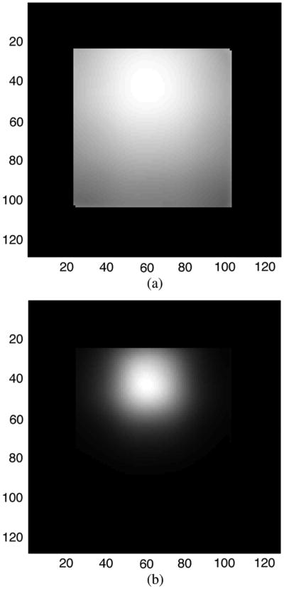
(a) Likelihood map for a sample event. The map was produced by computing the log-likelihood function at all MDRF points using the event’s nine PMT values. The likelihood map shown here has been zero-padded out to the nearest factor of two. White corresponds to high likelihoods. (b) The same likelihood map as shown in (a) but raised to a higher power. This transformation has been undertaken purely for illustrative purposes to make the algorithm’s searching methods more clear in a later figure.

The key to the search algorithm lies in computing only a fraction of the likelihood values shown on the likelihood map [14]. We begin by defining a grid of sixteen evenly-spaced test points on the zero-padded likelihood map as shown in Fig. 4(a). The likelihood is computed at these sixteen points. The maximum is found and a new grid is defined centered on that maximum value. The separation of the points in a new grid is half that of the previous grid, although the contraction rate can be made slower for estimation problems with more complicated likelihood maps. This process is repeated for the fixed number of iterations required to make the grid spacing match the pixel spacing.

Fig. 4.

A series of likelihood maps for a given event. The asterisks indicate the locations at which likelihoods will be computed at each iteration for this particular event. Note that a more peaked version of the likelihood map has been displayed for illustrative purposes.

The gradual homing in on the maximum-likelihood value and use of overlapping coordinate locations from iteration to iteration mean that the algorithm has a built-in error tolerance. For example, if the maximum-likelihood location selected from the initial sixteen coordinate locations is far from the true value (due to local features in the likelihood map), the algorithm allows the coordinate locations to migrate toward the true peak value over the course of its operation.

The pixels in the “zero-padded” region are actually assigned likelihoods beyond the range of possible values defined by the outputs of the system A/D converters, ensuring that the algorithm will never attempt to place the event in one of these virtual pixels. The motivation for the zero-padding is algorithm speed. By zero-padding, we are able to avoid conditional statements when determining each set of coordinate locations to test. Conditional statements slow software, prevent pipelining and parallel processing, and are difficult or impossible to implement in hardware. Employing a factor of two grid reduction method enables the use of simple pointer arithmetic with additions (and subtractions) to assign coordinate locations relative to the new grid center. This method for determining coordinate locations is viable and fast in both software and hardware. Fig. 4(b) demonstrates the necessity of the zero-padding to allow the division-of-two grid reduction for test locations near the edge of the camera face. Fig. 4 illustrates the substantial reduction in computation provided by the search algorithm. An exhaustive search would require 79 * 79 = 6241 computation whereas the grid search requires only 16 * 6 = 96 computations, several of which are zero multiplications.

E. Likelihood Windowing

Several techniques exist for determining whether a given set of PMT outputs resulted from a scattered photon or an unscattered photon. Three such techniques include energy windowing, likelihood windowing, and Bayesian windowing [15], [16]. Energy windowing and Bayesian windowing rely on separate computation of an energy estimate for the incident photon. We will not discuss those two methods of filtering.

Scattered events constitute noise in the data collected by a gamma camera. Likelihood windowing provides a natural method by which to eliminate scatter events when performing maximum-likelihood position estimation. In likelihood windowing, after the ML estimate of incidence location for an event has been calculated, the event’s likelihood value is compared to a likelihood threshold. If the likelihood for the event exceeds the threshold, the event is retained and added to the image [17].

Likelihood thresholds are calculated using the list-mode MDRF calibration data. After generating a mean file, position estimation is performed on the MDRF data as if it were an acquired image. The likelihood values for all events binned into a given pixel are then sorted. A pixel’s likelihood threshold is determined as the likelihood value in that pixel that achieves a desired event-acceptance rate. For example, with a 5000 event MDRF and a desired event-acceptance rate of 60%, the 3000th largest likelihood value in each pixel would be set as its likelihood threshold.

There are penalties associated with likelihood windowing, including the loss of counts as with any filtering procedure. However, since likelihoods have already been computed for the position estimation, there is minimal extra cost in computing time.

F. Comparison to Other Methods

Several alternative search methods exist for performing ML position estimation with conventional multipurpose CPU processing. This section will briefly address several of these methods, including exhaustive search, subset search, nested search, directed search, and lookup tables.

The performances of the contracting-grid search algorithm, directed search, and LUT with directed search methods were compared in terms of speed and the percentage correct with respect to the gold standard (exhaustive search). Flood data comprising two million events was used and computations were performed on a 2.0GHz processor (AMD Athlon MP 2400+) with 1.0GB of memory. In this 2D performance comparison, a parameter space of 79 × 79 was used. A performance summary for the different methods is shown in Table I. Percentage correct was calculated using both all possible events (no windowing of any kind) and also events accepted by both methods in question with likelihood windowing. For the parameters used in this study, the contracting-grid search method performed best in terms of percentage correct but was the slowest algorithm. However, this rank-ordering in terms of speed may change for detectors with more pixels because techniques like directed search and LUT become cumbersome with increases in pixel number or dimension. For example, the number of possible combinations of PMT signals in the cameras described above is N = 2^9*12 = 2¹⁰⁸. This number is so large that the use of lookup tables for these cameras is unfeasible, even with the use of data compression techniques. In the case of directed search algorithms, increased pixel number can result in a convergence time increasingly dependent on the initial evaluation position. The contracting-grid search algorithm requires only one more iteration (evaluation of 16 likelihood locations) for each factor 4 increase in detector area.

TABLE I.

Performance Comparison of Different ML Search Schemes Implemented in Conventional Computing Hardware

Search Method	Events/Second	Percent Acceptance	Percent Correct
			All Events	Accepted Events
Brute-force	2,257	86.9957	-	-
Directed	61,270	86.9738	99.12	99.77
LUT plus directed	85, 777	86.9731	98.99	99.71
Grid-Search	46,618	86.9784	99.43	99.85

One final but significant shortcoming of all of the alternative methods is the difficulty of implementing them in hardware. True real-time position estimates need to be a part of the data-acquisition electronics. The ability to implement this algorithm in hardware represents one of its greatest strengths.

IV. Algorithm Implementation

A. Imaging in Software

A need for real-time projection data motivated the development of this new algorithm. However, full hardware implementation represents a long-term goal. As a short-term solution and first step towards final hardware implementation, the algorithm has been successfully incorporated into the Center for Gamma-Ray Imaging’s (CGRI’s) current LabView data-acquisition software. On a standard CPU, the algorithm is computationally slower than some other methods, but algorithm speed is sufficient to allow the software to perform position estimation on a significant fraction of the incoming data, presenting the user with regularly-refreshed projection images of the object’s radiotracer source distribution. Further, upon collection of final data sets, the software presents the user with corresponding projection images within seconds of acquisition. The latest version of the software includes likelihood-windowing capability. Likelihood windowing slows the software slightly, but is qualitatively invaluable, particularly for low-count imaging applications. These tools have proven indispensable to the successful collection of data for real biomedical studies on the FastSPECT II system [18].

B. Hardware Implementation in FPGAs

The search algorithm has been carefully tailored to allow it to be built into hardware—an attribute lacking in the other ML position-estimation techniques described above. The goal of the hardware implementation of the position-estimation algorithm is to append position estimation data to raw data packets as they are transmitted to the back-end electronics.

In order to achieve high performance, a pipeline structure is employed. The pipeline works similarly to a shift register. As illustrated in Fig. 6, by staggering the clock values on which memory reads are performed, six sets of sixteen position estimates each may be computed simultaneously with five intermediate and one final position estimate returned for each of the six stages with every clock cycle (there is a short lag upon the initial arrival of events as the first event works its way through the pipeline).

Fig. 6.

A flow chart outlining the pipeline structure to be used for implementing the position estimation algorithm into hardware. The pipeline structure allows for position estimation to be performed simultaneously on several events despite the time constraints imposed by the necessary memory reads.

The first device chosen for trial hardware implementation of the contracting-grid search algorithm was an Orca Series 3 OR3T125B352 field-programmable system chip (FPSC). The chip is mounted on a board that contains several other components, including two static memories (SRAMs), a 33 MHz oscillator, general purpose LEDs, dual-inline-package (DIP) switches, and various probe and card connectors. The FPSC was programmed using VHDL via the Leonardo Spectrum software in the MentorGraphics suite of tools. Orca Foundry software was used for mapping and place-and-route. After writing the subsequent bitmap onto the chip, LabView software was used for testing.

The ORCA 3 chip used for programming was not large enough for full implementation of the algorithm with all six iterative steps. However, two VHDL designs were synthesized as proof-of-principle demonstrations that the algorithm is implementable in hardware. The first design computes a full log-likelihood, including log-factorial terms, for a 9-PMT modular camera. The second design computes two likelihoods in parallel.

C. 2D ML Position Estimation on a PLAYSTATION 3 Console

The Sony PLAYSTATION 3 (PS 3) console includes the Cell/BE processor, a powerful yet inexpensive processing unit that has been widely applied for scientific computation [19]–[26]. The Cell processor consists of a power processing element (PPE) and eight synergistic processing elements (SPEs). The PPE is used for general-purpose operations and to launch threads on the SPEs. Each SPE contains a synergistic processing unit (SPU), 256 KB of fast, on-chip memory (local store) and the logic to implement direct memory access (DMA) data transfers between main memory and local stores. Of the eight SPEs present in the Cell of the Sony PS 3, only six are available for external programming.

The 2D ML position estimation algorithm was successfully implemented using the following approach. Original event data are divided into six partitions, one partition for each PPE. Each PPE acquires its designated data partition and a portion of the necessary calibration data via DMA transfer. Because of the 256 KB size limit of the local store, only subsections of the calibration data may be stored at one time. A compromise between performance, memory constraints, and programming complexity is achieved by locally storing calibration data for each of the first three iterations of the algorithm. Calibration data for the remaining iterations are fetched as needed. Because objects tend to be centered in the object space field of view (FOV), calibration data for pixels near the detector center are used more often than data for pixels near the detector edge. Therefore, local store memory space was allocated across the SPEs for storage of calibration data corresponding to a 44 × 44 region in the detector center. This local storage method allows SPE-to-SPE DMA transfers for retrieval of the more frequently used detector center calibration data. Calibration data outside of the central 44 × 44 region are stored in main memory and accessed via memory-to-SPE DMA transfers. The intermediate values needed to implement the maximum search described by (1) are computed using vector floating point operations.

The Cell implementation was compared to an implementation written for a conventional cluster machine. The cluster machine code can process approximately 108,000 events per second when run on an AMD Opteron Processor 270 (2 GHz clock frequency, 1 MB cache size). The Cell code was compiled using the IBM XL C/C++ compiler, version 9.0 and can process approximately 1,012,000 events per second on a PS 3.

D. 3D ML Position Estimation on a GPU Supercomputer

The contracting-grid algorithm is extendable to multiple dimensions and was previously implemented for a 3D ML search task [27]. The algorithm was run on a graphics processing unit (GPU) supercomputer equipped with four NVIDIA GeForce 9800 GX2 graphics cards. The system configuration closely resembles the one developed at the Vision Lab, University of Antwerp, Belgium.

Because of its high performance and mass production, GPU hardware is revolutionizing scientific computing. A desktop machine capable of approximately 4 TFLOPS can be assembled at a total cost not exceeding <??? >3000. Consequently, many research projects now use GPU hardware [28]–[33]. The computational model is based on fine-grain threads, which share resources and cooperate with each other to carry out a complex task. An extension of the C/C++ programming language called CUDA (Compute Unified Device Architecture) allows the programmer to access the massively parallel computational power of GPUs and define threads to be run on any CUDA-enabled GPU device.

In the CUDA programming model, threads are grouped into ID, 2D, or 3D thread blocks. These thread blocks are grouped to form a ID or 2D grid. Threads in the same thread block can share a small amount (usually 16 KB) of fast on-chip memory. GPU engines are also equipped with off-chip memory, which, in the case of the NVIDIA GeForce 9800 GX2 card, comprises 1 GB. GPU engines typically have a few hundred simple cores, each capable of executing a single thread. Built-in variables store block and thread indexes, which are used by the thread to determine those elements of the input and/or output data on which it is to operate. Threads are handled automatically by the hardware, so that their generation and scheduling is extremely efficient. Thousands of threads can be generated/scheduled at the same in just a few clock cycles, diminishing the effect of memory latency since memory transfers and computation occur at the same time for different threads. For example, the execution of a thread that is about to perform a memory access will be suspended during the memory transfer, while another thread that already has data available for use will be selected for execution.

In the CUDA 3D ML implementation, a 69 × 69 × 25-voxel detector is considered. Each event is represented by the output of 64 MAPMT anodes [27]. The contracting grid algorithm is extended to the 3D case by considering a 4 × 4 × 4 grid instead of the 4 × 4 grid described for the 2D case above. Each event is assigned to a 4 × 4 × 4 thread block. Each thread in the thread block loads one of the 64 MAPMT outputs for the current event. This datum is copied to the shared memory where it may be accessed by all other threads in the thread block. Each thread in the thread block computes one of the likelihood values of the grid according to (3). Note that the fact that the number of MAPMT outputs (64) equals the number of grid points (4 × 4 × 4) is a fortunate coincidence that allows for this efficient thread usage. The location in the 3D grid at which the maximum likelihood value occurs is calculated and the grid contracted, as described above.

For comparison purposes, the 3D contracting grid algorithm was also implemented on a conventional machine. The conventional implementation was run on a system equipped with an AMD Phenom 9850 processor (2.5 GHz clock frequency, 512 KB cache size), resulting in the processing of approximately 1000 events per second. The CUDA implementation was capable of processing approximately 246,000 events per second when all GPU cards in the system were used.

V. Summary

An iterative search algorithm capable of operating in a multidimensional space and well-suited for hardware implementation was presented. The algorithm was developed to provide a fast means of determining the maximum-likelihood position estimate of an incident gamma ray upon the face of a scintillation camera. The algorithm may also prove useful in such applications as wavefront sensing, multidimensional position estimation, and pulse amplitude and timing. The algorithm was shown to have accuracy equal to or better than alternative search methods, to be applicable to complicated problems, and to easily extended to multiple dimensions. Also, the algorithm has been developed to allow for implementation in hardware, a feature lacking in other ML position estimation approaches. A general approach for the hardware implementation procedure in FPGAs was introduced and successful proof-of-principle trials were conducted in a small gate array. A 2D version of the algorithm was successfully implemented in the Cell processor of a Sony PLAYSTATION 3, resulting in event processing capabilities exceeding one million events per second. A 3D version of the algorithm was successfully implemented in a four-GPU system using CUDA, resulting in 3D event processing capabilities of almost 250,000 events per second compared to 1000 events per second on a conventional computer system. The algorithm is currently in use on several imaging systems at the CGRI.

Fig. 5.

(a) Flood image generated without likelihood windowing. The outer ring of pixels has been truncated. (b) Flood image generated with a 60% likelihood window. The outer ring of pixels has been truncated.

References

- 1.Barrett HH, Myers KJ. Foundations of Image Science. Hoboken, NJ: Wiley; 2004. [Google Scholar]
- 2.Barrett HH, Hunter WCJ, Miller BW, Moore SK, Chen Y, Furenlid LR. Maximum-likelihood methods for processing signals from gamma-ray detectors. IEEE Trans Nucl Sci. 2009 Jun;56(3):725–735. doi: 10.1109/tns.2009.2015308. [DOI] [PMC free article] [PubMed] [Google Scholar]
- 3.Hestenes MR, Steifel E. Methods of conjugate gradient for solving linear systems. J Res Nat Bureau Standards. 1952;49:309–436. [Google Scholar]
- 4.Knuth D. Sorting and Searching. 2. Vol. 3. Reading, MA: Addison-Wesley; 1998. The Art of Computer Programming. [Google Scholar]
- 5.Audet C, Dennis JJE. Mesh adaptive direct search algorithms for constrained optimization. SIAM J Optimization. 2006;17:188–217. [Google Scholar]
- 6.Conn AR, Scheinberg K, Vicente LN. Introduction to Derivative-Free Optimization, ser. MPS-SIAM Series on Optimization. Philadelphia, PA: SIAM; 2008. [Google Scholar]
- 7.Kolda TG, Lewis RM, Torczon V. Optimization by direct search: New perspectives on some classical and modern methods. SIAM Rev. 2003;45:385–482. [Google Scholar]
- 8.Sambridge MS, Kennett BLN. Seismic event location: Nonlinear inversion using a neighbourhood algorithm. Pure Appl Geophys. 2001;158:241–257. [Google Scholar]
- 9.Kennett BLN, Brown DJ, Sambridge MS, Tarlowski C. Signal parameter estimation for sparse arrays. Bulletin Seismological Soc Amer. 2003;93(4):1765–1772. [Google Scholar]
- 10.Hunter WCJ. PhD dissertation. Univ. Arizona; Tempe: 2007. Modeling stochastic processes in gamma-ray imaging detectors and evaluation of a multi-anode PMT scintillation camera for use with maximum-likelihood estimation methods. [Google Scholar]
- 11.Milster TD, Selberg L, Barrett H, Easton R, Rossi G, Arendt J, Simpson R. A modular scintillation camera for use in nuclear medicine. IEEE Trans Nucl Sci. 1984 Feb;31(1):578–580. [Google Scholar]
- 12.Sain JD. PhD dissertation. Univ. Arizona; Tempe: 2001. Optical modeling, design optimization, and performance analysis of a gamma camera for detection of breast cancer. [Google Scholar]
- 13.Chen Y-C, Furenlid LR, Wilson DW, Barrett HH. Small-Animal SPECT Imaging. ch 12. New York: Springer; 2005. pp. 195–201. [Google Scholar]
- 14.Furenlid L, Hesterman J, Barrett HH. Real-time data acquisition and maximum likelihood estimation for gamma cameras. Proc. 14th IEEE-NPSS Real Time Conf; 2005. pp. 498–501. [DOI] [PMC free article] [PubMed] [Google Scholar]
- 15.Chen J. PhD dissertation. Univ. Arizona; Tempe: 1995. Modular cameras: Improvements in scatter rejection and characterization and initial clinical application. [Google Scholar]
- 16.Chen JC. Scatter rejection in gamma cameras for use in nuclear medicine. Biomed Eng Appl, Basis Commun. 1997;9(20–26) [Google Scholar]
- 17.Chen J, Barrett H. Likelihood window, energy window, and Bayesian window for scatter rejection in gamma cameras. Proc. Nucl. Sci. Symp. Med. Imag. Conf; 1993. pp. 1414–1416. [Google Scholar]
- 18.Furenlid LR, Wilson DW, Chen YC, Kim H, Pietraski PJ, Crawford MJ, Barrett HH. FastSPECT II: A second-generation high-resolution dynamic SPECT imager. IEEE Trans Nucl Sci. 2004 Jun;51(3):631–635. doi: 10.1109/TNS.2004.830975. [DOI] [PMC free article] [PubMed] [Google Scholar]
- 19.Kahle JA, Day MN, Hofstee HP, Johns CR, Maeurer TR, Shippy D. Introduction to the cell multiprocessor. 2005;49(4/5):589–604. [Google Scholar]
- 20.Pham D, Aipperspach T, Boerstler D, Bolliger M, Chaudhry R, Cox D, Harvey P, Harvey P, Hofstee H, Johns C, Kahle J, Kameyama A, Keaty J, Masubuchi Y, Pham M, Pille J, Posluszny S, Riley M, Stasiak D, Suzuoki O, Takahashi M, Warnock J, Weitzel S, Wendel D, Yazawa K. Overview of the architecture, circuit design, and physical implementation of a first-generation cell processor. 2006 Jan;41(1):179–196. [Google Scholar]
- 21.Hofstee P. Introduction to the cell broadband engine. IBM Corporation; Riverton, NJ: 2005. [Google Scholar]
- 22.Williams S, Shalf J, Oliker L, Kamil S, Husbands P, Yelick K. The potential of the cell processor for scientific computing. Proc. 3rd Conf. Comput. Frontiers; New York. 2006. pp. 9–20. [Google Scholar]
- 23.Bader DA, Agarwal V, Madduri K, Kang S. High performance combinatorial algorithm design on the cell broadband engine processor. 2007;33(10/11):720–740. [Google Scholar]
- 24.Benthin IWC, Scherbaum M, Friedrich H. Ray tracing on the cell processor. Proc. IEEE Symp. Interactive Ray Trac; Sep. 2006; pp. 15–23. [Google Scholar]
- 25.Sakamoto M, Murase M. Parallel implementation for 3-D CT image reconstruction on Cell Broadband Engine. Proc. IEEE Int. Conf. Multimedia Expo; Jul. 2007; pp. 276–279. [Google Scholar]
- 26.Kachelrieß M, Knaup M, Bockenbach O. Hyperfast parallel-beam and cone-beam backprojection using the cell general purpose hardware. 2007 Apr;34(4):1474–1486. doi: 10.1118/1.2710328. [DOI] [PubMed] [Google Scholar]
- 27.Hunter W, Barrett HH, Furenlid LR. Calibration method for ML estimation of 3D interaction position in a thick gamma-ray detector. 2009 Feb;56(1):189–196. doi: 10.1109/TNS.2008.2010704. [DOI] [PMC free article] [PubMed] [Google Scholar]
- 28.Pratx G, Chinn G, Olcott PD, Levin CS. Fast, accurate and shift-varying line projections for iterative reconstruction using the GPU. 2009 Mar;28(3):435–445. doi: 10.1109/TMI.2008.2006518. [DOI] [PMC free article] [PubMed] [Google Scholar]
- 29.Samant SS, Xia J, Muyan-Ozelik P, Owens JD. High performance computing for deformable image registration: Towards a new paradigm in adaptive radiotherapy. 2008 Aug;35(8):3546–3553. doi: 10.1118/1.2948318. [DOI] [PubMed] [Google Scholar]
- 30.Bi W, Chen Z, Zhang L, Xing Y. Accelerate helical cone-beam CT with graphics hardware. In: Hsieh J, Samei E, editors. Med Imag: Phys Med Imag; Proc. SPIE; Mar, 2008. p. 69132T. [Google Scholar]
- 31.Vetter C, Westermann R. SPECT reconstruction on the GPU. In: Hsieh J, Samei E, editors. Med Imag: Phys Med Imag; Proc. SPIE; Mar, 2008. p. 69132R. [Google Scholar]
- 32.Rossler F, Botchen RP, Ertl T. Dynamic shader generation for GPU-based multi-volume ray casting. 2008 Sept./Oct;28(5):66–77. doi: 10.1109/MCG.2008.96. [DOI] [PubMed] [Google Scholar]
- 33.Schiwietz T, Chang TC, Speier P, Westermann R. MR image reconstruction using the GPU. In: Flynn MJ, Hsieh J, editors. Med Imag: Phys Med Imag; Proc. SPIE; Mar, 2006. p. 61423T. [Google Scholar]