

Abstract
We have investigated the sensitivity of two-dimensional infrared (2D IR) spectroscopy to peptide helicity with an experimental and theoretical study of Z-[L-(αMe)Val]8-OtBu in CDCl3. 2D IR experiments were carried out in the amide-I region under the parallel and the double-crossed polarization configurations. In the latter polarization configuration, the 2D spectra taken with the rephasing and nonrephasing pulse sequences exhibit a doublet feature and a single peak, respectively. These cross-peak patterns are highly sensitive to the underlying peptide structure. Spectral calculations were performed on the basis of a vibrational exciton model, with the local mode frequencies and couplings calculated from snapshots of molecular dynamics (MD) simulation trajectories using six different models for the Hamiltonian. Conformationally variant segments of the MD trajectory, while reproducing the main features of the experimental spectra, are characterized by extraneous features, suggesting that the structural ensembles sampled by the simulation are too broad. By imposing periodic restraints on the peptide dihedral angles with the crystal structure as a reference, much better agreement between the measured and the calculated spectra was achieved. The result indicates that the structure of Z-[L-(αMe)Val]8-OtBu in CDCl3 is a fully developed 310-helix with only a small fraction of α-helical or nonhelical conformations in the middle of the peptide. Of the four different combinations of pulse sequences and polarization configurations, the nonrephasing double-crossed polarization 2D IR spectrum exhibits the highest sensitivity in detecting conformational variation. Of the six local mode frequency models tested, the electrostatic maps of Mukamel and Cho perform the best. Our results show that the high sensitivity of 2D IR spectroscopy can provide a useful basis for developing methods to improve the sampling accuracy of force fields and for characterizing the relative merits of the different protocols for the Hamiltonian calculation.
I. Introduction
Helices are important elements of protein secondary structure associated with a variety of structural and functional properties in biological systems.1–4 The three types of helices found in nature, the 310-helix, the α-helix, and the π-helix, are different in their hydrogen bonding patterns, having i ← i + 3, i ← i + 4, and i ← i + 5 hydrogen bonding, respectively.5,6 Of these, the α-helix is the most abundant species. The 310-helix often occurs at the termini of helical segments in naturally occurring proteins7 and is thought to be a folding intermediate in the formation of α-helices from nascent random coils of amino acids.8,9 Chemical environments and other factors that promote either of these two helical forms or a reversible dimorphism between the two have been discussed in recent studies.10–14 It has been proposed that interconversion between the α- and 310-helical forms can have important biological consequences, such as in the pore opening mechanism of channel proteins.15 To elucidate the roles of different helices and their possible transformations, it is necessary to develop highly sensitive techniques that can report subtle changes accompanying helical transitions, which is challenging. Although the different helical types differ in the mean values of dihedral angles, there is some structural overlap between them, reflected in overlapping regions of the Ramachandran space.
Femtosecond two-dimensional infrared (2D IR) spectroscopy of the amide-I mode (primarily C=O stretch) has been shown to be a powerful probe of peptide structures.16–20 Couplings between amide-I modes, manifested as cross-peaks in 2D IR spectra, are highly sensitive to backbone conformations. Compared to conventional techniques, such as electronic circular dichroism (ECD) and NMR, the intrinsic picosecond time resolution of 2D IR makes it particularly attractive because it can be utilized to probe ultrafast folding/unfolding processes.21 Although time-resolved linear IR has provided very valuable information on protein folding kinetics, it is impossible to resolve the different types of helices that may be involved in the helix–coil transition using linear IR. 2D IR studies of unlabeled amide-I modes have demonstrated its capabilities in distinguishing between 310- and α-helical octapeptides,22,23 probing the onset of 310-helical secondary structure,24 and revealing the cross-peaks between the A and E modes of a 21-residue α-helix.25 Isotope edited helical peptides with 13C and 13C/18O on the amide-I modes and 15N on the amide-II mode were also targeted by the 2D IR technique to gain insights into residue-specific structural information.26,27 Further investigation on the sensitivity of 2D IR to peptide helicity is, thus, a very timely and important next step.
To firmly establish the 2D IR spectrum–structure relationship, translation of the measured complex spectra into accurate descriptions of secondary structure requires input from theoretical models. Molecular dynamics (MD) simulation provides a space–time trajectory, which can be used in conjunction with theoretical methods to extract structural and dynamical information that can be compared to experimental data. A number of studies utilized solvent configurations generated from MD snapshots to parametrize electrostatic models that describe how the frequency of an amide-I vibrator depends on its local environment.28–33 Several applications of these and related models have been pursued to simulate 2D IR experimental data and evaluate the effects of solvent and ensemble heterogeneity in 2D IR spectra.34–36
In this work, we investigate the sensitivity of 2D IR to peptide helicity using a combination of experimental and molecular simulation approaches. The system of our study is the terminally protected homo-octapeptide, Z-[L-(αMe)Val]8-OtBu (Z, benzyloxycarbonyl; (αMe)Val, Cα-methyl valine; OtBu, tert-butoxy, Figure 1), solvated in CDCl3. We have chosen to focus on a peptide with an uncoded Cα-tetrasubstituted amino acid because such amino acids are well-known to have high propensity toward helical conformations as a result of the steric hindrances imposed by the substituents.37–40 The conformational stability of Cα-tetrasubstituted peptide systems makes them excellent models for developing experimental and theoretical approaches to conformational analysis. Among these systems, Z-[L-(αMe) Val]8-OtBu is of particular interest. It adopts a fully developed, right-handed 310-helical conformation in the crystal state.41,42 Previous ECD, VCD, and 2D IR experiments concluded that it forms a stable 310-helix in CDCl3, but undergoes acidolysis of the terminal OtBu group and a subsequent 310-to-α-helix transition in 1,1,1,3,3,3-hexafluoropropan-2-ol.22,43,44 This interesting feature will provide a platform for detailed investigation of helix stability and transformation in different solvents.
Figure 1.
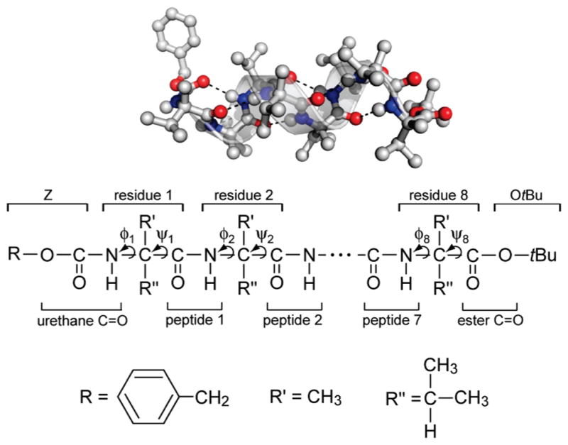
Z-[L-(αMe)Val]8-OtBu with its helical ribbon superimposed (top). The backbone 310-helical hydrogen bonds are shown in dashed lines. Chemical identities of constituent groups (bottom).
Previously, we have reported the 2D IR cross-peak pattern of Z-[L-(αMe)Val]8-OtBu in CDCl3 using the rephasing (R) pulse sequence with the double-crossed polarization configuration.22 The doublet cross-peak pattern in the amide-I region was assigned as a characteristic of the 310-helical conformation, as corroborated by our theoretical calculations.23 Here, we present 2D spectra taken by two different pulse sequences, R and nonrephasing (NR), under both the parallel and the double-crossed polarization configurations. These experiments together with linear IR provide an extensive set of spectral signatures for comparison with theoretical simulations. The comparison also allows us to explore the relative sensitivity of different polarization configurations and pulse sequences to the underlying peptide structure.
To gain a deeper insight into the conformational distribution of this peptide and to go beyond the simple assumptions made in the previous work that the peptide backbone dihedral angles follow Gaussian distributions centered at either the same average values or the crystal structure,23 we have performed all-atom MD simulations to obtain structural ensembles with and without restraints. We simulated 2D IR spectra based on the vibrational exciton model16 and calculated the amide-I local mode frequencies using six different models based on four electrostatic maps recently developed by the Cho,29,45 Keiderling,31 Knoester,46,47 and Mukamel48 groups. Through detailed comparison with the experimental data, the performance of the adapted MD force field in generating realistic peptide structures is analyzed. The relative efficacies of different models in simulating 2D spectra are explored and discussed. We find that 2D IR spectra are exquisitely sensitive to small changes in structural characteristics of helices and can serve as a stringent test for force field refinement and theoretical model development.
II. Methods
A. Experiment
Details of the 2D IR spectrometer along with the data acquisition and processing procedure have been described elsewhere.22,23 Briefly, the 2D IR measurements were carried out using 100-fs IR pulses with a center frequency of 1667 cm−1 and wavevectors of ka, kb, and kc. The delay time between the first and second incoming pulses is denoted as τ; that between the second and third pulses, as T; and that after the arrival of the third pulse, as t. The third-order nonlinear signal emitted in the phase-matching direction of −ka + kb + kc was combined with a local oscillator field and heterodyne-detected. Pulse sequences of a-b-c and b-a-c are defined as R and NR, respectively. The R and NR 2D spectra were collected with the parallel (〈Z, Z, Z, Z〉) and double-crossed (〈π/4, −π/4, Y, Z〉) polarization configurations, where 〈a, b, c, d〉 denotes the polarization of the excitation pulses (a, b, c) and the signal (d). It has already been shown that this polarization configuration is effective in structural discrimination of helices.23 All experiments were performed at ambient temperature (20 °C). The 310-helix octapeptide Z-[L-(αMe)Val]8-OtBu was synthesized and characterized by Toniolo and co-workers, as described previously.42 The peptide concentration in CDCl3 (Cambridge Isotope Laboratories, 99.96% D) is ~10 mM. The peak optical density of the amide-I mode is ~0.3 in a 100-μm-thick sample cell.
B. Force Field Adaptation and Molecular Dynamics Simulations
The NAMD package49 was used for all the simulations in this study. The crystal structure of Z-[L(αMe)Val]8-OtBu41 was used as the initial configuration for our MD simulations, performed with a modified CHARMM22 force field.50 The CHARMM force field has been widely used in the conformational sampling of helices and in calculating free energy changes associated with their formation, and the results have been found to be largely consistent with experiments.51–54 However, the default CHARMM force field does not provide partial charges and bond parameters for Cα-tetrasubstituted amino acids, or the Z and OtBu capping groups. Although a previous study utilized CHARMM to perform energy minimization on a singly-(αMe)Val-substituted peptide and found that Cα-tetrasubstitution leads to a decrease in conformational flexibility,55 no details of the force field adaptation were given. In this work, we have assigned partial charges as consistent as possible with the CHARMM force field. The modular form of neutral subgroups available in this force field is highly advantageous to our purposes. In CHARMM, the HN–CαH in each amino acid is assigned partial charges of (0.31e, −0.47e, 0.07e, 0.09e), respectively; the amide C=O is assigned partial charges of (0.51e, −0.51e), respectively; and the methyl and methylene groups belonging to hydrophobic amino acid residues are, in general, assigned partial charges such that they form neutral groups with charges of 0.09e on the H atoms. To maintain an overall neutral charge for the HN–Cα–CH3 groups, we assigned the atoms with partial charges of 0.31e (amide H), −0.47e (amide N), 0.16e (Cα), −0.27e (methyl C), and 0.09e (methyl H). Within the Z group, the urethane carbonyl group (partial charges of 0.63e and −0.52e for C and O, respectively) and the ester oxygen (partial charge −0.34e) were adapted from the topology of dimyristoylphosphatidylcholine (DMPC) available in CHARMM27,56 and the phenyl group was directly adapted from the topology of the phenylalanine residue. To maintain charge neutrality, the carbon and the hydrogen atoms of the methylene group of Z were assigned partial charges of 0.05e and 0.09e, respectively. The carbonyl group of the eighth residue and the ester oxygen in the OtBu group were treated in the same manner as those in the Z group. The partial charges of the methyl groups in OtBu were adapted according to the neutral methyl groups of hydrophobic amino acid residues, and the carbon atom that connects the three methyl groups was assigned a partial charge of 0.23e to maintain neutrality. The adaptation also reflected the atom type of each atom, and the bonded parameters were assigned accordingly from the force field.
There are several models of chloroform available in the literature.57–59 In this study, we have adopted the chloroform parameters from the AMBER force field.60 We have verified that an equilibrated box of chloroform yields the correct density, diffusion coefficient, and radial distribution functions when compared to existing data.57
The peptide was solvated with 968 CDCl3 molecules in a rectangular box measuring about 50.9 Å × 52.4 Å × 52.6 Å. After 1000 steps of conjugate gradient energy minimization, two sets of simulations, unrestrained (u) and restrained (r), were performed to obtain the spectra. To obtain the unrestrained simulation, a 200 ps positionally restrained simulation was first performed at a pressure of 1 atm and a temperature of 295 K, with the peptide backbone atoms harmonically restrained to the crystal structure coordinates with a force constant of 1 kcal mol−1 Å−2. The restraints were then lifted, and the system was equilibrated to attain a constant pressure and temperature for 8.65 ns. The trajectory u was a constant energy trajectory generated for 30 ns during which the temperature fluctuation was quite small with a 1.3 K standard deviation. To monitor conformational evolution, the spectra were calculated for three segments taken from u, which were labeled u1 (0–2 ns), u2 (10–12 ns), and u3 (22–24 ns). To obtain the restrained r simulation, the system was first equilibrated at a constant pressure of 1 atm and a temperature of 295 K. During this period, harmonic positional restraints of 2 kcal mol−1 Å−2 were first applied to the peptide non-hydrogen atoms for 200 ps, followed by restraints of 1 kcal mol−1 Å−2 on the backbone heavy atoms for 3.4 ns. Subsequently, the r simulation was performed at constant energy for 2 ns duration, with the (φ, ψ) torsional angles of the peptide restrained in a periodic potential using the peptide crystal structure as the reference. A force constant of 75 kcal mol−1 radian−2 was used to restrain the angles, except for the floppier terminal residues (specifically, φ1, ψ1, and ψ8 in Figure 1) for which a force constant of 95 kcal mol−1 radian−2 was applied. During all equilibration runs, constant temperature was maintained using Langevin dynamics with a collision frequency of 1 ps−1. The Nosé–Hoover Langevin Piston algorithm61,62 was used to maintain constant pressure. Bond lengths involving hydrogen atoms were held fixed with the SHAKE algorithm.63 A time step of 1 fs was used to integrate the equations of motion, and three-dimensional periodic boundary conditions were applied to the orthorhombic simulation cell. Electrostatic interactions were calculated using the particle mesh Ewald sum.64 The nonbonded cutoff distance was set at 11 Å, and the van der Waals interactions and real space part of the Ewald sum were smoothly truncated over the interval 10–11 Å. Coordinates were saved every 0.1 ps in both the u and r production runs.
C. Calculation of Spectra with the Vibrational Exciton Model
The vibrational exciton model is combined with a sum-over-states approach to calculate the amide-I linear and 2D IR spectra.16 In the vibrational exciton model, the amide-I modes of a peptide are considered to be coupled oscillators that give rise to a set of one- and two-quantum excitonic states, with the number of single excitonic states being equal to the number of oscillators. With the application of laser pulses, the system undergoes transitions between excitonic states. The spectra are calculated from the trajectories in the static limit, assuming that the time scales of fast and slow motions are clearly separated. The total Hamiltonian, H, has a diagonal contribution, H0, due to local mode frequencies; a coupling contribution between neighboring peptide units, V1; and a contribution due to the interaction of non-neighboring units, V2:
| (1) |
The local mode frequencies in H0 are obtained from model calculations that take into account electrostatic effects of solvent molecules and peptide atoms on individual sites. Several groups have recently created DFT electrostatic maps that correlate the amide-I local mode frequencies to either the electrostatic potential29,31 or the components of the electrostatic field vector, their gradients,46 and second derivatives48 at the individual sites. Most of the maps utilize N-methylacetamide (NMA) and the nitrogen-deuterated form (NMA-d) as models for the local peptide unit. The effects of fluctuating environments are modeled either by solvent clusters obtained from molecular dynamics snapshots,31,28 or by imposing external electric fields of varying configurations.46,48 In this work, we have taken four of these maps combined with two variations to come up with six different models for calculating the local mode frequencies, as summarized in Table 1. In naming the models, we distinguish between the potential (P) and field (F) based models using the second letter of the model name. For each model, the definition of parametrized atoms (red) for individual sites is shown together with a collection of atoms surrounding them. This complete group of atoms has a zero net charge and is defined as the chromophore. Atoms within a given chromophore are excluded from the calculations of electrostatic effects of that chromophore.
TABLE 1.
Summary of the Models Used for Spectral Calculationsa
| Model | Electrostatic map | Parametrized sites and chromophor definition (i = 1 to 7) | Nearest neighbor coupling map |
|---|---|---|---|
| CP1 | Cho29 |  |
Cho29 |
| CP2 | |||
| KP | Keiderling31 |  |
Cho29 |
| KF1 | Knoester46 | 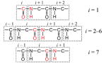 |
Knoster47 |
| KF2 | Knoester46 | 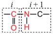 |
Knoester47 |
| MF | Mukamel48 |  |
Cho29 |
Parametrized atoms are shown in red. The red shading in the MF model schematically indicates the transition charge region for sampling.
For the electrostatic potential-based models, the frequency shift at the ith amide-I local mode (δωi) from the gas-phase frequency (ω0) is given by
| (2) |
Here, and represent, respectively, the potentials due to the solvent and the peptide at the kth parametrized atom of the ith mode, and ck represents the parameters that convert the electrostatic potentials at the kth atom to the frequency shift. A particular mode contains N such parametrized atoms that are shown in Table 1 in red. The atoms whose electrostatic contributions are counted include the solvent atoms and the peptide atoms that lie outside the chromophore definition.
The four-site electrostatic potential map developed by Cho and co-workers parametrized the fitting parameters ck using NMA–nD2O (n = 1–5) complexes.29 They also obtained partial charges for the four parametrized sites (C, O, N, H) on the basis of various dipeptide and tripeptide conformations.45 The frequency origin was set to ω0 = 1707 cm−1, a calculated value for the NMA amide-I mode. We have calculated the linear and IR spectra using this potential map, both with (CP1) and without (CP2) using the parametrized partial charges in the electrostatic calculation. For these models, the ith chromophore includes the (C=O) atoms of the ith residue and the (HN–Cα) atoms of the consecutive residue. To maintain charge neutrality in the CP1 model, the Cα atom within the chromophore is assigned a zero charge.
The KP model is based on the ck parameters reported by Bouř and Keiderling,31 which were obtained on the basis of NMA-d in variable-sized D2O clusters with 0–31 water molecules. The parametrized sites within the ith chromophore for this model are the (Cα–C=O) atoms of the ith residue and the nitrogen atom of the consecutive residue, and ω0 = 1732 cm−1, the calculated gas-phase frequency for NMA-d at the BPW91/6-31G** level.31 To ensure charge neutrality, we have included the (NH) atoms of the i residue and the H and Cα atoms of the next residue in the chromophore definition.
The KF models are based on the electrostatic field-gradient map reported by Jansen and Knoester.46 This map linearly correlates the frequency shift with the electrostatic field (Ekα) and gradient (Ekαβ) by
| (3) |
In their parametrization, NMA-d was subjected to 74 different point-charge environments and ω0 = 1717 cm−1, the gas phase frequency of NMA-d measured by resonance Raman spectroscopy.65 Jansen et al. also performed Hessian reconstruction on the normal modes of Ac-Gly-NHMe (nitrogen-deuterated), and reported nearest-neighbor frequency shift (NNFS) maps.47 From these maps, the frequency shifts due to the neighboring peptide units can be obtained as a function of the instantaneous (φ, ψ) dihedral angles between each peptide unit and its nearest neighbors. The KF1 model described in Table 1 uses the electrostatic map for the non-nearest neighboring peptide atoms and the NNFS maps for the contributions of the nearest-neighboring residues. For the terminal amide modes, the NNFS shifts can be obtained from only a single neighbor because such maps for the effects of capping groups are not available. To understand and compare the relative merit of the NNFS map, we have also calculated the spectra purely on the basis of the electrostatic map. The chromophore definition for this model, described as KF2 in Table 1, is identical to the chromophore definition of the CP models.
The MF model employs the map48 implemented in the SPECTRON package created by Zhuang et al.66 Similar to the KF electrostatic map, this map was constructed by amide-I frequency calculations of a single NMA molecule subject to a set of nonuniform multipole electric fields with ω0 = 1728 cm−1. However, the amide-I frequency shift and anharmonicity were parametrized as a linear plus a quadratic function of the electrostatic vector that contains 19 components of the electric field and its gradients and second derivatives. The parametrization sampled over 67 points in the transition charge region of the peptide unit. The segment made of the amide residue and two neighboring neutral groups containing the Cα is defined as the chromophore.
For the CP1, CP2, KP, and MF models, we obtained the nearest-neighbor coupling term, V1, from the instantaneous dihedral angles, using the ab initio map provided by Cho.29 For the KF1 and KF2 models, the coupling map of Knoester was used.47 The coupling contribution of the non-nearest neighboring peptide units, V2, was approximated by the transition dipole coupling interactions67,68 using a previous parametrization of the magnitude, position, and orientation of the dipoles.45 For the two-quantum Hamiltonian, the diagonal anharmonicity of each local mode was set to 16 cm−1, an experimental value measured for NMA-d. The couplings between these states were considered to be bilinear under the harmonic approximation.16
Linear and 2D IR spectra were obtained by diagonalizing the one- and two-excition Hamiltonians and calculating the frequency domain response functions. In the impulsive limit with well-separated pulses, the linear spectrum S(ω) and the 2D complex spectra for the R and NR pulse sequence, SR(ωτ, ωt; T) and SNR(ωτ, ωt; T), can be represented as follows:
| (4) |
| (5) |
| (6) |
Here, i and j represent the one-exciton states, and k represents the two-exciton states. The transition frequency between the ground and one-exciton states is ωi, and that between the one-and two-exciton states is ωki = ωk − ωi. The angle brackets represent the ensemble average over the inhomogeneous conformational distribution. The isotropically averaged orientation factors, On, account for the effect of the relative polarization directions of the pulses in the four-wave mixing experiment. The factors for parallel polarization 2D data with T ≠ 0 can be found in previous studies.69,70 For the R spectrum taken with the double-crossed polarization at T = 0, two different pulse sequences, a-b-c and a-c-b, contribute to the signal, and the corresponding orientation factors have been reported earlier.23 For the NR spectrum taken with the double-crossed polarization at T = 0, two different pulse sequences, b-a-c and b-c-a, contribute to the signal:
| (7) |
| (8) |
The corresponding orientation factors, On, are shown in Table 2. In our calculations, the homogeneous dephasing rate constants γ and γ′ for the 0–1 and 1–2 transitions were taken to be 4.5 and 6 cm−1, respectively. These values were chosen to represent the typical Lorentzian line width for the amide-I band as well as to take into account deviations from the harmonic approximation for the higher quantum states, as detailed earlier.23
TABLE 2.
Orientation Factors for the Double-Crossed Polarization <π/4, −π/4, Y, Z > Configuration
| Pulse Sequence | Orientation factor | ||
|---|---|---|---|
| b-a-c |
|
0 | |
|
|
− |μi|2|μj|2 + (μi · μi)2 | ||
|
|
− (μi · μjk)(μj · μik) + (μi · μik)(μj · μjk) | ||
| b-c-a |
|
− (μi · μj)(μik · μkj) + (μi · μik)(μj · μjk) | |
|
|
− (μi · μjk)(μj · μik) + (μi · μik)(μj · μjk) | ||
The calculated linear and 2D IR spectra are shown in Figures 4, 5, and 7. Because the amide-I local mode frequency shifts obtained from the six different models are quite different in their magnitudes (Figure 8), the calculated linear spectra have been shifted to coincide with the amide-I peak position in the experimental linear IR spectrum to enable a direct comparison of the spectral features. The shift for each model calculation is given at the upper right corner of the linear IR spectrum. The same shift is applied to the two frequency axes of the corresponding 2D spectrum. Because we set the frequency origin, ω0, of each model on the basis of the values in the original references, this shift is a measure of how closely each model can predict the experimental peak position.
Figure 4.

Normalized linear and 2D IR spectra for the u1, u2, and u3 segments of the unrestrained trajectory, calculated with the CP2 model. The number in the upper right corner of the FT IR spectrum panel indicates the frequency shift (in cm−1) applied to the calculated spectra.
Figure 5.

Normalized linear and 2D IR spectra for the u1, u2, and u3 segments of the unrestrained trajectory calculated with the MF model. The number in the upper right corner of the FT IR spectrum panel indicates the frequency shift (in cm−1) applied to the calculated spectra.
Figure 7.

The linear and 2D IR spectra calculated with the CP1, CP2, KP, KF1, KF2, and MF models for the restrained trajectory r. The number in the upper right corner of the FT IR spectrum panel indicates the frequency shift (in cm−1) applied to the calculated spectra.
Figure 8.

The amide-I local mode frequency shifts calculated with the CP1, CP2, KP, KF1, KF2, and MF models for the trajectory r. Blue circles, solvent contributions ( ); red circles, peptide backbone and side chain contributions ( ); black circles, total shifts ( ). The vertical bars indicate the range enclosed by ±1 standard deviation (σi). Green symbols with solid and dash lines in KF1 are the NNFS and electrostatic contributions in , respectively.
III. Results and Discussions
A. The Experimental Spectra
Figure 2 shows the FT IR and absolute magnitude 2D spectra of Z-[L-(αMe)Val]8-OtBu in CDCl3. In the FT IR spectra, the peak corresponding to the amide-I band is observed at 1659 cm−1. The smaller peak centered near 1720 cm−1 is attributed to two unresolved bands corresponding to urethane and ester C=O groups located at the N and C termini. Additionally, there is a marginal shoulder present in the vicinity of 1680 cm−1.
Figure 2.

The experimentally measured spectra from left to right: FT IR; rephasing, parallel polarization; nonrephasing, parallel polarization; rephasing, double-crossed polarization; nonrephasing, double-crossed polarization.
The 2D IR spectra obtained with the R pulse sequence are elongated along the diagonal due to spectral inhomogeneity. On the other hand, the NR spectra are elongated equally along both the ωt and ωτ directions. These general features are common to spectra obtained both in the parallel and the double-crossed polarization configurations. 2D spectra in the double-crossed polarization configuration effectively lead to a cancellation of the diagonal peaks, thereby revealing the cross peaks of lower intensity. The normalized NR spectrum in this polarization configuration has a single intense peak. The intense doublet of peaks in the R spectrum has been noted as a signature of significant presence of 310-helicity in the sample.23 The main features of the spectra are due to the overall vibrational excitonic band that arises from a combination of individual excitonic states and their couplings. Although it is not possible to attribute details of the spectral features to properties of individual excitonic states, it has been observed that the overall amide I spectra change in response to changes in the overall secondary structure.23 In the following sections, we discuss our findings on the response of the 2D IR spectra to small changes in structural characteristics of Z-[L-(αMe)Val]8-OtBu as indicated by analysis of MD simulation trajectories. In addition, we will utilize the sensitivity of this experimental method as a benchmark for force field accuracy and for judging the effectiveness of various methods of spectral calculations.
B. Performance of the Force Field
In Figure 3a, we show the structural evolution of the peptide backbone based on interresidue hydrogen bonding during the course of the unrestrained simulation, u. The hydrogen bonding has been determined on the basis of the Kabsch–Sander energy criterion,71 and the data have been averaged over blocks of 500 ps. The cutoff value for the hydrogen bond energy is taken to be −0.5 kcal mol−1. This criterion allows up to a 63° misalignment for the ideal H-bond length of 2.9 Å and a N-to-O distance of up to 5.2 Å for perfect alignment, and makes it possible for a residue to simultaneously have both 310- and α-helical hydrogen bonding. As expected, the degree of disorder is the greatest near the termini: the urethane C=O group and the amide C=O on the fifth residue exhibit nonhelical conformations for a significant fraction of the simulated time, even though they can be hydrogen bonded to residues 3 and 8, respectively, to assume a 310-helical conformation. Greater ordering is found between residues 1–4. The first and second amide C=O groups spend a greater time in forming a 310-helical hydrogen bond. The third and fourth residues show a substantial fraction of α-helical hydrogen bonding as well as some bifurcated 310- and α-helical hydrogen bonding.
Figure 3.

Hydrogen bonding pattern for (a) trajectory u, averaged over blocks of 500 ps, and (b) trajectory r averaged over blocks of 100 ps. Red, 310-helix; blue, α-helix; magenta, both 310- and α-helices; green, nonhelical configuration. The u1 (0–2 ns), u2 (10–12 ns), and u3 (22–24 ns) segments are marked with broken lines.
The hydrogen bonding data show that the conformational space described by the adapted CHARMM force field evolves over tens of nanoseconds. There is a distinct change in the peptide structure between about 7 and 17 ns, with an increase in the 310-helicity in the middle residues, and a simultaneous decrease in 310-helicity for the terminal regions. The disorder in the urethane C=O persists even after 17 ns. Overall, there is relatively higher preference for 310-helicity over α-helicity in the entire peptide. The segments u1 (0–2 ns), u2 (10–12 ns), and u3 (22–24 ns) have been selected from the three conformationally distinct segments of trajectory u.
To understand how peptide conformational changes affect spectral features, we show in Figures 4 and 5 the linear and 2D IR spectra of three segments of varying structure taken from the unrestrained trajectory. These spectra have been calculated on the basis of two methods (models CP2 and MF in Table 1) judged best for spectral calculations (discussed in following subsections). In the linear spectra calculated with the MF model, there is an appearance of a shoulder close to the region of the actual shoulder found in the experimental spectrum. However, the shoulder in the calculated spectrum for u2 is significantly stronger than the experiment. With the CP2 model, there is slight variation in the line shape of the linear spectra from u1 to u3 with no significant changes in the line width.
We next observe the effect of changing conformations on the 2D spectra calculated in the parallel polarization. The R spectra obtained with CP2 show a single peak and are essentially featureless for all three segments. Although the NR spectra obtained with CP2 also have a single peak, there is a slight splitting of the peak in the u1 segment. Overall, the conformational changes that occur with time evolution of the trajectory do not strongly affect these spectra. Similar to the linear spectrum, the R spectra obtained with the MF model show some effect of the conformational change that takes place in the unrestrained segments. The single, broad peak in u1 is split in u2, and the splitting decreases in u3. The NR spectrum obtained with MF, on the other hand, captures the changes in conformations more sensitively. There is a small peak splitting in the u1 spectrum, which progressively becomes more pronounced from u2 to u3. Thus, the NR spectrum in the parallel polarization scheme is relatively more effective in capturing the effects of structural changes than the R spectrum.
The changes observed in the calculated spectra from the u1 to u3 segments are more distinct in the double-crossed polarization configuration. With the MF model, the R spectrum exhibits the doublet peak pattern in u1 with a small protruding shoulder in the lower diagonal half of the peak doublet. This shoulder becomes progressively stronger in the u2 and u3 trajectory segments and splits from the doublet. The NR spectra with this method show a distinct peak splitting. The splitting is the most pronounced in u2, and the relative intensity of the lower-frequency peak is the weakest in u3. The R spectrum obtained with the CP2 model is very similar in appearance to the corresponding experimental spectrum. The only noticeable signature of the conformational change from u1 to u3 is the gradual appearance of a protruding peak in the lower diagonal doublet. This peak is similar to the peak found in the MF spectra, but is of much lower intensity and does not split from the main peak. The effect of conformational change is seen more clearly in the NR spectra obtained with the CP2 method. The relative positions and intensities of two split peaks vary substantially between different segments.
For all the trajectory segments, the linear and 2D IR spectra simulated with both methods have some degree of qualitative agreement with the corresponding experimental spectra, with the main features of the experimental spectra appearing in the calculated spectra. However, the calculated spectra exhibit some extraneous features that are absent in the experimental data. Although the line shapes of the linear and the parallel polarization spectra show clear differences from the experiment, the effect of the conformational changes is best captured by the spectra in the double-crossed polarization configuration. The appearance of an extra peak accompanying the lower diagonal peak in the R doublet and the distinct peak splitting in the NR spectra are different from the experimental results. Thus, the simulation clearly shows that the double-crossed polarization is more effective in distinguishing conformational evolution in a sample. Further, within the data obtained with a particular polarization configuration, the NR spectrum appears to be more sensitive to conformational changes than the R spectrum.
The results discussed above suggest that the conformational sampling obtained from the u simulation, although inclusive of the conformations present in the experimental sample, may be too broad. To gain further insight into the conformational preferences of the force field, we show in Figure 6b–d the Ramachandran plots for u1, u2, and u3. The dihedral angles are time averages over the segments and the standard deviations of the dihedrals are given in Table 3. Also shown is the Ramachandran plot of the peptide crystal structure. A statistical analysis of crystal structures of peptides containing at least one Cα-tetrasubstituted α-amino acid shows that the average dihedral angles (φ, ψ) is (−63°, −42°) for the α-helix and (−57°, −30°) for the 310-helix.5 However, significant variations have been reported,5 and one study reports different average values for 310-helices found in proteins.7 To estimate the range of typical backbone fluctuations, we took the measured value of 0.85 for the square of the NMR order parameter for secondary structure elements72 and calculated a standard deviation of about ±11° (shown as a box of side 22° centered at the mean dihedral angles of 310-helix in Figure 6). Although most residues in the unrestrained trajectory exhibit average dihedral angles that are within the box defining 310-helicity, a few tend to move to the edge or lie outside the range. The terminal residues tend to be farther away from the 310-helical conformations than the residues at the center of the peptide. The ψ8 angle of the last residue (Figure 1) lies well outside the 310-defining range. The φ1 angle is positive for the unrestrained simulations, at great variance with the corresponding angle of the crystal structure and outside of the range of Figure 6.
Figure 6.

Ramachandran plots of the peptide amino acid residues: (a) the crystal structure;41 (b) trajectory u1; (c) u2; (d) u3; and (e) r. The dihedral values plotted are time averages. The number corresponds to the residue number in Figure 1. The ψ8 angle is defined on the basis of the N–C–C–O dihedral angle, with the O atom being the ester oxygen associated with the OtBu group. The dashed box indicates the range of ±11° centered at (φ, ψ) = (−57°, −30°).
TABLE 3.
Average Dihedral Angles and Their Standard Deviations (in parentheses), for the Unrestrained Trajectories u1, u2, and u3, and the Dihedrally Restrained Trajectory ra
| crystal structure |
u1 |
u2 |
u3 |
r |
||||||
|---|---|---|---|---|---|---|---|---|---|---|
| i | φi | ωi | φi | ωi | φi | ωi | φi | ωi | φi | ωi |
| 1 | −56.8 | −32.6 | 61.7 (11.7) | −86.8 (13.9) | 53.1 (36.9) | −77.2 (19.1) | 64.1 (10.2) | −83.2 (13.2) | −55.8 (5.3) | −33.2 (4.9) |
| 2 | −51.9 | −25.0 | −56.3 (11.4) | −28.7 (10.4) | −59.6 (10.2) | −17.9 (17.3) | −59.8 (9.6) | −18.9 (14.6) | −51.9 (5.4) | −22.6 (5.2) |
| 3 | −55.7 | −23.8 | −48.9 (10.8) | −35.0 (11.9) | −61.7 (9.5) | −15.7 (11.2) | −61.4 (9.7) | −19.2 (12.4) | −55.6 (5.2) | −28.4 (5.3) |
| 4 | −50.6 | −30.8 | −51.1 (10.4) | −40.0 (8.9) | −51.9 (9.1) | −36.7 (8.3) | −52.4 (9.4) | −37.9 (9.1) | −53.1 (5.3) | −34.8 (5.3) |
| 5 | −50.5 | −35.1 | −55.3 (9.5) | −45.8 (8.2) | −57.0 (8.4) | −28.6 (8.2) | −51.9 (10.1) | −44.7 (8.4) | −54.4 (5.5) | −41.4 (5.3) |
| 6 | −49.1 | −39.3 | −59.5 (9.6) | −38.8 (9.6) | −63.0 (8.9) | −39.6 (9.9) | −58.0 (9.6) | −38.9 (9.3) | −54.5 (5.7) | −40.1 (5.8) |
| 7 | −62.3 | −33.9 | −64.9 (9.4) | −44.0 (8.9) | −64.9 (9.5) | −45.3 (9.2) | −64.8 (9.2) | −44.0 (8.8) | −64.4 (5.7) | −38.4 (5.7) |
| 8 | −62.4 | −58.0 | −60.6 (9.2) | −66.4 (10.7) | −60.6 (9.1) | −65.7 (10.5) | −61.1 (9.1) | −66.2 (10.3) | −63.5 (5.6) | −60.9 (5.2) |
The dihedral angles for the peptide crystal structure41 are also listed.
C. Restrained Simulations and Performance of Different Electrostatic Approaches
As seen in the previous section, comparison of the theoretically calculated 2D IR spectra with the experimental results suggests that the conformational space sampled by the unrestrained simulation, while largely coincident with the 310-helix region, has some degree of variance with conformations in the actual experimental ensemble. Since peptides with the L-(αMe)Val group are reported to be biased toward the 310-helical conformation73 and since the crystal structure of the Z-[L-(αMe)Val]8-OtBu peptide is within the 310-helical boundaries (as seen in Figure 6a), we decided to simulate this peptide in CDCl3 by restraining its dihedral angles near the crystal structure values. Figure 3b shows the H-bonding characterization of the restrained trajectory, r, time-averaged over blocks of 100 ps. The residues satisfy an entirely 310-helical H-bonding pattern for more than 50% of the trajectory snapshots. Unlike the unrestrained trajectory, the urethane C=O and the first residue are characterized by an absence of nonhelical configurations, and the fifth residue has a significantly greater fraction of 310 helicity. A minor presence of α-helicity is noticed at the middle of the peptide, mainly at the fourth residue. The population of conformations that belong to neither helix type is much less than that observed for the unrestrained simulation. The Ramachandran plot in Figure 6e shows that the peptide structure is well within the limits of the 310-helical conformation. The standard deviations of the dihedral angles are roughly half the corresponding values for the unrestrained simulation, indicating a lesser extent of structural heterogeneity.
The trajectory r has a large degree of conformational similarity to the peptide crystal structure. To understand the extent to which these conformations are representative of the conformations of Z-[L-(αMe)Val]8-OtBu solvated in CDCl3, the linear and 2D spectra have been calculated for this trajectory using the six models in Table 1 and are reported in Figure 7. It has been shown that the local mode frequencies in H0 are the most important contribution to the Hamiltonian that significantly affect the spectra.29,34 The restrained trajectory presents an opportunity to judge the relative merits of the various electrostatic approaches for calculating the frequency shift.
The first two rows compare the effects of using the partial charges from the Cho model versus the partial charges from the force field. The linear spectra do not show any noticeable changes. Considering the 2D parallel polarization data, the R spectra obtained with CP1 and CP2 are very similar, whereas the NR spectrum obtained with the CP2 model is slightly broader. The differences between the models can be discerned mainly from the appearance of the double-crossed polarization 2D spectra. Although the R spectra obtained with both models are very similar to the experiment, the NR spectrum obtained with CP1 shows a more prominent splitting of the main peak than CP2. The spectra obtained with the CP2 method agree more closely with the experiment than those obtained with CP1. This suggests that more accurate estimates of the frequency shifts may be obtained from the electrostatic calculations that use the same charges as those used in propagating the simulation trajectories.
Spectra computed using the KP model are shown in the third row in Figure 7. Although the linear spectrum and the R spectra obtained in both the parallel and the double-crossed polarization configurations agree well with the corresponding experimental measurements, there are distinct discrepancies between the calculated and measured NR spectra. The NR spectra in both polarization configurations show extraneous features in the main peak with the double-crossed polarization spectrum showing a distinct splitting. Interestingly, the linear spectrum and the R spectra obtained in both polarization configurations with the KP model show strong similarities to the corresponding data obtained with the CP2 model. Differences between these models become more apparent upon inspection of the NR data. The NR spectra obtained with KP in both polarization configurations are distinctly broader than both the spectra obtained with CP2 and the corresponding experimental spectra. This suggests that the NR pulse sequence has higher sensitivity for comparing different protocols of spectral calculations.
The fourth and the fifth rows in Figure 7 show, respectively, the results obtained with the electrostatic field-gradient models KF1 and KF2, thereby comparing the effects of using the shifts obtained with the NNFS map. The linear and the parallel polarization 2D spectra obtained with the KF1 model are much broader than the corresponding experimental spectra. With the double-crossed polarization, the R spectrum consists of a small protrusion in the lower diagonal peak doublet, which is stronger than the similar feature seen in the corresponding CP1 spectrum. However, the double-crossed NR spectrum exhibits a single main peak and agrees well with the experiment. With the KF2 model, there is good agreement with experiment for the linear spectrum, as well as for the R spectra in both polarization configurations. The NR spectra obtained in both polarization configurations, although closer to a single main peak compared with other models, are too broad when compared with the corresponding experimental results. Inspection of all the spectra together indicates that for the system under consideration, usage of only the electrostatic map (KF2) yields better agreement with experiment than when the electrostatic and NNFS maps are used together (KF1).
The last row shows the results obtained with the MF model. The spectra from this model are narrower than the corresponding spectra obtained by the other potential and field/gradient methods. The linear spectrum is somewhat narrower than the experiment, but the parallel polarization R and NR spectra show very good agreement with experiment. The double-crossed polarization R spectrum shows the peak doublet without extraneous features, whereas the NR spectrum shows a shoulder at the higher frequency side of the main peak.
The spectra calculated from the trajectory r using CP2 and MF give an overall better agreement with the experiment than the spectra calculated for the different segments of the trajectory u. The line shapes obtained are simultaneously reasonable for all spectra, and the peak splitting as well as the presence of extraneous spectral features observed in the NR spectrum is marginal. Comparing all the calculated spectra for r, the agreement with the experiment is good for the parallel polarization configuration, but the differences are more distinct when the 2D double-crossed polarization spectra are considered. Unlike the R spectra obtained for the unrestrained segments, the protruding peak in the lower diagonal peak of the doublet is not prominent, except for the KF1 model. The splitting of the NR peak is similarly negligible, except for with the CP1 and KP models. Due to the better agreement of the calculations with experiment, we believe that the conformations of the trajectory r are a good representation of the actual structural ensemble of Z-[L-(αMe)Val]8-OtBu peptide solvated in CDCl3 at room temperature. On the basis of this trajectory, the CP2 and MF models appear to be the best approaches among the six for spectral calculation for this system. For both models, the experimental peak doublet of the R spectrum in the double-crossed polarization method, proposed as a signature of 310 helicity,23 is well-reproduced. The line broadening of the lower diagonal peak in the doublet is comparable to the experimental line broadening, as is its intensity relative to the stronger upper peak (0.58 for CP2; 0.66 for MF; 0.60 in the experiment). The double-crossed polarization NR spectra exhibit a slight but acceptable splitting. The parallel polarization NR spectrum from the MF model gives a single peak with a line width comparable to the experiment.
To more closely compare the models and get further insight into their similarities and differences, we show in Figure 8 the mean values of local mode frequency shifts ( ) and their standard deviations (σi), separated into the electrostatic contributions from the solvent ( ) and from the peptide atoms outside the chromophore ( ). It is interesting to note the high degree of similarity between the solvent shifts obtained with different models, both in the magnitude and in the trend of variations across the peptide backbone. Greater fluctuation in the solvent shifts is found at the terminal peptide units than those found in the middle of the peptide. All models show a greater shift at the sixth and seventh modes, consistent with greater solvent exposure of the last two peptide units at the peptide C terminus. Analysis of the radial distribution functions reveals that ~40% of the snapshots exhibit a solvent deuterium atom within 3 Å of the O atom of the second peptide unit, but the percentage is less than 5% for the first, third, and fourth units, and ~30% for the fifth unit. Thus, the solvent-induced frequency shift of the second unit is relatively large. The similarity in the solvent shifts reflects the similarity in the approaches in creating the electrostatic maps: by mapping the electrostatic effect of surrounding solvent molecules or external fields onto the amide-I mode of the NMA or NMA-d molecule.
As seen in Figure 8, the differences between are more significant than those of . Obviously, the differences in the values obtained with CP1 and CP2 are due to dissimilar partial charges used in the two models. It is interesting to note that the trends in the peptide shifts (not the absolute values) are very similar between the CP2, KP, and KF2 models, all of which use the partial charges of the force fields in the shift calculation. Although the KF1 model uses the same partial charges, the difference in the trends can be attributed to the NNFS contributions. Because the NNFS maps are not available for the capping groups, the first and the last peptide units are assigned with a different chromophore definition from the middle units (Table 1), and of these two units become much smaller in magnitude. The large variation in the KF1 local mode frequencies results in the much broader line shape in the calculated linear and 2D IR spectra. It is clear from these results that calculating the NNFS maps for the capping groups will be essential for the proper application of the KF1 model to short peptides.
Figure 9 shows and σi of the CP2 and MF models for the unrestrained trajectories u1–u3. Comparing to the result for the trajectory r in Figure 8, the σi of CP2 in the unrestrained simulation are, on average, 13% higher and can reach 30% higher at some residues. The larger frequency fluctuations in the unrestrained trajectory are not unexpected because the larger standard deviations in the dihedral angle distributions (Table 3) can lead to greater variations in the local environment that individual peptide units experience. However, the calculated linear and 2D R spectra of u1–u3 are only slightly broader than r. The widths of the calculated spectra do not follow the trend of the σi; that is, the inhomogeneous distributions of individual peptide units. Rather, they depend on the relative spread of . This behavior is also observed in the MF model. The u2 segment has the largest spread, and its linear and 2D R spectra exhibit a distinctly higher frequency shoulder and splitting, even though the σi do not show a specific trend compared to r. The results suggest that accurate modeling of local mode frequency shifts is essential for proper simulation of linear and 2D IR lineshapes.
Figure 9.

The amide-I local mode frequency shifts calculated with the CP2 and MF models for unrestrained trajectories u1–u3. Circles indicate the mean values ( ). The vertical bars indicate the range enclosed by ±1 standard deviation (σi).
All models require a red shift of the simulated spectra to overlap with the experiment (Figure 7). Presumably, one major contribution to the necessary red shifts comes from the fact that the dispersion forces are important in CDCl3 but are not taken into account in the pure electrostatic maps. In a previous simulation of NMA in CDCl3 using the GROMOS87 force field and the KF electrostatic map, the predicted frequency was too high by 29 cm−1.46 This shift may account for a systematic error in solvent contribution to the 44 cm−1 shift of the KF2 model, because the KF map is, in principle, transferable between force fields. Another study of the same system using the AMBER parm99 force field and a six-site electrostatic potential map28 predicted a 15 cm−1 blue shift from the experiment.74 This shift is similar to those of CP1 and CP2, although the force field and map used in that study are different from this study. Neglecting polarization effects in the MD force field could also contribute to the blue shift of simulated spectra.
Although the experimental linear spectrum exhibits a low-frequency wing that is not reproduced by the six model simulations, the full width at half maximum of the simulated linear spectra and the diagonal width of the simulated parallel 2D R spectra are comparable to, or just slightly wider than, the experimental data, with the exception of KF1, which is much broader (probably due to the lack of NNFS maps for the capping groups, as discussed earlier), and MF, which is somewhat narrower. This behavior is in contrast to the observation in some previous studies34,75 that the line width obtained from field-based models is significantly larger than that obtained from potential-based models. Moreover, although our simulated spectra were static averages over MD snapshots, we do not observe significant broadening of the simulated line width compared to the experiment, as was observed in a similar MD study on a 12-residue β-hairpin, a 19-residue α-helix, and a 76-residue α + β protein.34 It has been shown that motional narrowing effects are important for properly simulating the linear and nonlinear responses of NMA.32,46,48,66 For floppy, small peptides, the inclusion of dynamic effects may be important.76 Another MD simulation on a 22-residue polyalanine suggests that the line-broadening process can be approximately described by considering the inhomogeneous distribution of instantaneous normal-mode frequencies.77 Because the (αVal)Me octapeptide is quite structurally restrained due to Cα-methylation, it is unclear how significant the dynamic effects are. We will explore this topic in the future by other computational methods, such as the time-averaging approximation,78,79 and numerical integration of the Schrödinger equation.80
IV. Conclusions
The interplay between 2D IR experiments and spectral simulations performed in this study has demonstrated that 2D IR spectral patterns obtained with multiple pulse sequences and polarization configurations are highly sensitive to peptide secondary structure. The effects of different structural ensembles and different electrostatic models are more clearly revealed in the double-crossed polarization spectra than in the parallel polarization spectra due to the suppression of diagonal peaks. Within the same polarization configuration, the NR spectra exhibit higher sensitivity than the R spectra.
From our results, we can conclude that the solution structure of Z-[L-(αMe)Val]8-OtBu in CDCl3 is a fully developed 310-helix with a conformational distribution centered at the crystal structure. This is based on the good agreement with experimentally measured spectra achieved through model calculations using the restrained trajectory. Without the restraints, the CHARMM simulation force field, as adapted in the present study for Cα-methylated amino acids, samples a broader conformational space than the one encompassed by the conformations in our actual experimental sample. Comparing the six electrostatic models for predicting the amide-I local mode frequencies, the CP2 and MF models performed the best in reproducing the experimental spectral patterns, including the number of peaks and their relative positions and intensities. All six models yielded amide-I frequencies that are too high compared to the experiment. This discrepancy could be attributed to the strong dispersion forces of the solvent that are not taken into account in the electrostatic models.
Our results suggest that further improvements in the MD simulations and spectral calculations are needed to fully establish the spectra–structure relationship. It is evident that force field parameters need to be refined for accurate conformational sampling, at least for the short Cα-methylated peptides considered here. Some previous studies suggested that modern force fields behave comparably in predicting protein structural and dynamic properties.81 Others revealed significant differences among the force fields for the secondary-structure forming tendencies51 and unfolded peptide conformational distributions.82,83 The protocol adopted in this study can provide a basis for exploring the sampling accuracy of other force fields. For electrostatic models, the results from the CP and KP models might be further improved if we utilized the partial charges and structural ensemble generated by the same force field that was used for parametrization. This requires future simulation and testing. To apply NNFS maps in short peptides, it is necessary to generate maps for the capping groups. Although two of the electrostatic models perform quite well within the limit of static inhomogeneous averaging, the effect of vibrational dynamics on spectral patterns should be further explored using more advanced simulation protocols. The 2D IR technique, with its versatile variations of pulse sequences and polarizations, can provide large sets of spectral constraints that are very useful for stringent testing and validation of the next generation of force fields and theoretical models. With refinement, the interplay between 2D IR experiments and simulations will enable us to go beyond model systems and gain detailed insights into important biological problems, such as protein folding and aggregation.
Acknowledgments
This work was supported in part by the NIH (GM 59230 to S.M.) and NSF (CHE-0745892 to S.M., CHE-041758 and -0750175 to D.J.T., and CHE-0450045 to N.H.G.). We are grateful to Quirinius B. Broxterman (DSM Pharmaceuticals Products, Geleen, The Netherlands) for providing the L-(αMe)Val amino acid and to Yang Han for the analysis of radial distribution functions of solvent molecules.
References and Notes
- 1.Roux B, MacKinnon R. Science. 1999;285:100. doi: 10.1126/science.285.5424.100. [DOI] [PubMed] [Google Scholar]
- 2.Bussell R, Eliezer D. J Mol Biol. 2003;329:763. doi: 10.1016/s0022-2836(03)00520-5. [DOI] [PubMed] [Google Scholar]
- 3.Akitake B, Anishkin A, Liu N, Sukharev S. Nat Struct Mol Biol. 2007;14:1141. doi: 10.1038/nsmb1341. [DOI] [PubMed] [Google Scholar]
- 4.Sivaramakrishnan S, Spink BJ, Sim AYL, Doniach S, Spudich JA. Proc Natl Acad Sci USA. 2008;105:13356. doi: 10.1073/pnas.0806256105. [DOI] [PMC free article] [PubMed] [Google Scholar]
- 5.Toniolo C, Benedetti E. Trends Biochem Sci. 1991;16:350. doi: 10.1016/0968-0004(91)90142-i. [DOI] [PubMed] [Google Scholar]
- 6.Bolin KA, Millhauser GL. Acc Chem Res. 1999;32:1027. [Google Scholar]
- 7.Barlow DJ, Thornton JM. J Mol Biol. 1988;201:601. doi: 10.1016/0022-2836(88)90641-9. [DOI] [PubMed] [Google Scholar]
- 8.Millhauser GL. Biochemistry. 1995;34:3873. doi: 10.1021/bi00012a001. [DOI] [PubMed] [Google Scholar]
- 9.Shea JE, Brooks CL. Annu Rev Phys Chem. 2001;52:499. doi: 10.1146/annurev.physchem.52.1.499. [DOI] [PubMed] [Google Scholar]
- 10.Smythe ML, Huston SE, Marshall GR. J Am Chem Soc. 1995;117:5445. [Google Scholar]
- 11.Hungerford G, Marta MI, Birch DJS, Moore BD. Angew Chem Intl Ed. 1996;35:326. [Google Scholar]
- 12.Pengo P, Pasquato L, Moro S, Brigo A, Fogolari F, Broxterman QB, Kaptein B, Scrimin P. Angew Chem, Int Ed. 2003;42:3388. doi: 10.1002/anie.200351015. [DOI] [PubMed] [Google Scholar]
- 13.Bellanda M, Mammi S, Geremia S, Demitri N, Randaccio L, Broxterman QB, Kaptein B, Pengo P, Pasquato L, Scrimin P. Chem—Eur J. 2007;13:407. doi: 10.1002/chem.200600719. [DOI] [PubMed] [Google Scholar]
- 14.Crisma M, Saviano M, Moretto A, Broxterman QB, Kaptein B, Toniolo C. J Am Chem Soc. 2007;129:15471. doi: 10.1021/ja076656a. [DOI] [PubMed] [Google Scholar]
- 15.Long SB, Tao X, Campbell EB, MacKinnon R. Nature. 2007;450:376. doi: 10.1038/nature06265. [DOI] [PubMed] [Google Scholar]
- 16.Hamm P, Lim M, Hochstrasser RM. J Phys Chem B. 1998;102:6123. [Google Scholar]
- 17.Asplund MC, Zanni MT, Hochstrasser RM. Proc Natl Acad Sci USA. 2000;97:8219. doi: 10.1073/pnas.140227997. [DOI] [PMC free article] [PubMed] [Google Scholar]
- 18.Hochstrasser RM. Proc Natl Acad Sci USA. 2007;104:14190. doi: 10.1073/pnas.0704079104. [DOI] [PMC free article] [PubMed] [Google Scholar]
- 19.Cho M. Chem Rev. 2008;108:1331. doi: 10.1021/cr078377b. [DOI] [PubMed] [Google Scholar]
- 20.Zhuang W, Hayashi T, Mukamel S. Angew Chem, Int Ed. 2009;48:3750. doi: 10.1002/anie.200802644. [DOI] [PMC free article] [PubMed] [Google Scholar]
- 21.Hamm P, Helbing J, Bredenbeck J. Annu Rev Phys Chem. 2008;59:291. doi: 10.1146/annurev.physchem.59.032607.093757. [DOI] [PubMed] [Google Scholar]
- 22.Maekawa H, Toniolo C, Moretto A, Broxterman QB, Ge NH. J Phys Chem B. 2006;110:5834. doi: 10.1021/jp057472q. [DOI] [PubMed] [Google Scholar]
- 23.Maekawa H, Toniolo C, Broxterman QB, Ge NH. J Phys Chem B. 2007;111:3222. doi: 10.1021/jp0674874. [DOI] [PubMed] [Google Scholar]
- 24.Maekawa H, Formaggio F, Toniolo C, Ge NH. J Am Chem Soc. 2008;130:6556. doi: 10.1021/ja8007165. [DOI] [PubMed] [Google Scholar]
- 25.Woutersen S, Hamm P. J Chem Phys. 2001;115:7737. [Google Scholar]
- 26.Fang C, Wang J, Kim YS, Charnley AK, Barber-Armstrong W, Smith AB, Decatur SM, Hochstrasser RM. J Phys Chem B. 2004;108:10415. [Google Scholar]
- 27.Maekawa H, De Poli M, Toniolo C, Ge NH. J Am Chem Soc. 2009;131:2042. doi: 10.1021/ja807572f. [DOI] [PubMed] [Google Scholar]
- 28.Ham S, Kim JH, Lee H, Cho M. J Chem Phys. 2003;118:3491. [Google Scholar]
- 29.Ham S, Cho M. J Chem Phys. 2003;118:6915. [Google Scholar]
- 30.Ham S, Cha S, Choi JH, Cho M. J Chem Phys. 2003;119:1451. [Google Scholar]
- 31.Bouř P, Keiderling TA. J Chem Phys. 2003;119:11253. [Google Scholar]
- 32.Schmidt JR, Corcelli SA, Skinner JL. J Chem Phys. 2004;121:8887. doi: 10.1063/1.1791632. [DOI] [PubMed] [Google Scholar]
- 33.Watson TM, Hirst JD. Mol Phys. 2005;103:1531. [Google Scholar]
- 34.Ganim Z, Tokmakoff A. Biophys J. 2006;91:2636. doi: 10.1529/biophysj.106.088070. [DOI] [PMC free article] [PubMed] [Google Scholar]
- 35.Wang J, Zhuang W, Mukamel S, Hochstrasser RM. J Phys Chem B. 2008;112:5930. doi: 10.1021/jp075683k. [DOI] [PMC free article] [PubMed] [Google Scholar]
- 36.Lin YS, Shorb JM, Mukherjee P, Zanni MT, Skinner JL. J Phys Chem B. 2009;113:592. doi: 10.1021/jp807528q. [DOI] [PMC free article] [PubMed] [Google Scholar]
- 37.Marshall GR. In: Intra-Science Chemistry Reports. Kharasch N, editor. Gordon & Breach; New York: 1971. p. 305. [Google Scholar]
- 38.Paterson Y, Rumsey SM, Benedetti E, Némethy G, Scheraga HA. J Am Chem Soc. 1981;103:2947. [Google Scholar]
- 39.Karle IL, Balaram P. Biochemistry. 1990;29:6747. doi: 10.1021/bi00481a001. [DOI] [PubMed] [Google Scholar]
- 40.Toniolo C, Crisma M, Formaggio F, Valle G, Cavicchioni G, Précigoux G, Aubry A, Kamphuis J. Biopolymers. 1993;33:1061. doi: 10.1002/bip.360330708. [DOI] [PubMed] [Google Scholar]
- 41.Toniolo C, Polese A, Formaggio F, Crisma M, Kamphuis J. J Am Chem Soc. 1996;118:2744. [Google Scholar]
- 42.Polese A, Formaggio F, Crisma M, Valle G, Toniolo C, Bonora GM, Broxterman QB, Kamphuis J. Chem—Eur J. 1996;2:1104. [Google Scholar]
- 43.Yoder G, Polese A, Silva RAGD, Formaggio F, Crisma M, Broxterman QB, Kamphuis J, Toniolo C, Keiderling TA. J Am Chem Soc. 1997;119:10278. [Google Scholar]
- 44.Moretto A, Crisma M, Formaggio F, Kaptein B, Broxterman QB, Keiderling TA, Toniolo C. Biopolymers (Pept Sci) 2007;88:233. doi: 10.1002/bip.20680. [DOI] [PubMed] [Google Scholar]
- 45.Choi JH, Ham SY, Cho M. J Phys Chem B. 2003;107:9132. [Google Scholar]
- 46.Jansen TlC, Knoester J. J Chem Phys. 2006;124:044502. doi: 10.1063/1.2148409. [DOI] [PubMed] [Google Scholar]
- 47.Jansen TlC, Dijkstra AG, Watson TM, Hirst JD, Knoester J. J Chem Phys. 2006;125:044312. doi: 10.1063/1.2218516. [DOI] [PubMed] [Google Scholar]
- 48.Hayashi T, Zhuang W, Mukamel S. J Phys Chem A. 2005;109:9747. doi: 10.1021/jp052324l. [DOI] [PubMed] [Google Scholar]
- 49.Kale L, Skeel R, Bhandarkar M, Brunner R, Gursoy A, Krawetz N, Phillips J, Shinozaki A, Varadarajan K, Schulten K. J Comput Phys. 1999;151:283. [Google Scholar]
- 50.MacKerell AD, Jr, Bashford D, Bellott M, Dunbrack RL, Evanseck JD, Field MJ, Fischer S, Gao J, Guo H, Ha S, Joseph-McCarthy D, Kuchnir L, Kuczera K, Lau FTK, Mattos C, Michnick S, Ngo T, Nguyen DT, Prodhom B, Reiher WE, III, Roux B, Schlenkrich M, Smith JC, Stote R, Straub J, Watanabe M, Wiorkiewicz-Kuczera J, Yin D, Karplus M. J Phys Chem B. 1998;102:3586. doi: 10.1021/jp973084f. [DOI] [PubMed] [Google Scholar]
- 51.Yoda T, Sugita Y, Okamoto Y. Chem Phys Lett. 2004;386:460. [Google Scholar]
- 52.Yang AS, Honig B. J Mol Biol. 1995;252:351. doi: 10.1006/jmbi.1995.0502. [DOI] [PubMed] [Google Scholar]
- 53.Bu L, Im W, Brooks CL. Biophys J. 2007;92:854. doi: 10.1529/biophysj.106.095216. [DOI] [PMC free article] [PubMed] [Google Scholar]
- 54.Kokubo H, Okamoto Y. Chem Phys Lett. 2004;383:397. [Google Scholar]
- 55.He YB, Huang Z, Raynor K, Reisine T, Goodman M. J Am Chem Soc. 1993;115:8066. [Google Scholar]
- 56.Feller SE, MacKerell AD., Jr J Phys Chem B. 2000;104:7510. [Google Scholar]
- 57.Tironi IG, Van Gunsteren WF. Mol Phys. 1994;83:381. [Google Scholar]
- 58.Jorgensen WL, Maxwell DS, Tirado-Rives J. J Am Chem Soc. 1996;118:11225. [Google Scholar]
- 59.Norberg J, Nilsson L. Biophys J. 1998;74:394. doi: 10.1016/S0006-3495(98)77796-3. [DOI] [PMC free article] [PubMed] [Google Scholar]
- 60.Case DA, Cheatham TE, III, Darden T, Gohlke H, Luo R, Merz KM, Jr, Onufriev A, Simmerling C, Wang B, Woods RJ. J Comput Chem. 2005;26:1668. doi: 10.1002/jcc.20290. [DOI] [PMC free article] [PubMed] [Google Scholar]
- 61.Feller SE, Zhang Y, Pastor RW, Brooks BR. J Chem Phys. 1995;103:4613. [Google Scholar]
- 62.Martyna GJ, Tobias DJ, Klein ML. J Chem Phys. 1994;101:4177. [Google Scholar]
- 63.Ryckaert JP, Cicotti G, Berendsen HJC. J Comput Phys. 1977;23:327. [Google Scholar]
- 64.Essmann U, Perera L, Berkowitz ML, Darden T, Lee H, Pedersen LG. J Chem Phys. 1995;103:8577. [Google Scholar]
- 65.Mayne LC, Hudson B. J Phys Chem. 1991;95:2962. [Google Scholar]
- 66.Zhuang W, Abramavicius D, Hayashi T, Mukamel S. J Phys Chem B. 2006;110:3362. doi: 10.1021/jp055813u. [DOI] [PMC free article] [PubMed] [Google Scholar]
- 67.Krimm S, Bandekar J. Adv Protein Chem. 1986;38:181. doi: 10.1016/s0065-3233(08)60528-8. [DOI] [PubMed] [Google Scholar]
- 68.Torii H, Tasumi M. J Chem Phys. 1992;96:3379. [Google Scholar]
- 69.Hochstrasser RM. Chem Phys. 2001;266:273. [Google Scholar]
- 70.Wang J, Hochstrasser RM. Chem Phys. 2004;297:195. [Google Scholar]
- 71.Kabsch W, Sander C. Biopolymers. 1983;22:2577. doi: 10.1002/bip.360221211. [DOI] [PubMed] [Google Scholar]
- 72.Palmer AG., III Annu Rev Biophys Biomol Struct. 2001;30:129. doi: 10.1146/annurev.biophys.30.1.129. [DOI] [PubMed] [Google Scholar]
- 73.Mammi S, Rainaldi M, Bellanda M, Schievano E, Peggion E, Broxterman QB, Formaggio F, Crisma M, Toniolo C. J Am Chem Soc. 2000;122:11735. [Google Scholar]
- 74.DeCamp MF, DeFlores L, McCracken JM, Tokmakoff A, Kwac K, Cho M. J Phys Chem B. 2005;109:11016. doi: 10.1021/jp050257p. [DOI] [PubMed] [Google Scholar]
- 75.Hayashi T, Jansen TlC, Zhuang W, Mukamel S. J Phys Chem A. 2005;109:64. doi: 10.1021/jp046685x. [DOI] [PubMed] [Google Scholar]
- 76.Jansen TlC, Zhuang W, Mukamel S. J Chem Phys. 2004;121:10577. doi: 10.1063/1.1807824. [DOI] [PubMed] [Google Scholar]
- 77.Ham S, Hahn S, Lee C, Kim TK, Kwak K, Cho M. J Phys Chem B. 2004;108:9333. [Google Scholar]
- 78.Auer BM, Skinner JL. J Chem Phys. 2007;127:104105. doi: 10.1063/1.2766943. [DOI] [PubMed] [Google Scholar]
- 79.Jansen TlC, Wioletta MR. J Chem Phys. 2008;128:214501. [Google Scholar]
- 80.Jansen TlC, Knoester J. Biophys J. 2008;94:1818. doi: 10.1529/biophysj.107.118851. [DOI] [PMC free article] [PubMed] [Google Scholar]
- 81.Price DJ, Brooks CL., III J Comput Chem. 2002;23:1045. doi: 10.1002/jcc.10083. [DOI] [PubMed] [Google Scholar]
- 82.Hu H, Elstner M, Hermans J. Protein Struct, Funct, Bioinf. 2003;50:451. doi: 10.1002/prot.10279. [DOI] [PubMed] [Google Scholar]
- 83.Mu Y, Kosov DS, Stock G. J Phys Chem B. 2003;107:5064. [Google Scholar]