Meta-Analysis For Rare Events

SUMMARY

Meta analysis provides a useful framework for combining information across related studies and has been widely utilized to combine data from clinical studies in order to evaluate treatment efficacy. More recently, meta analysis has also been used to assess drug safety. However, because adverse events are typically rare, standard methods may not work well in this setting. Most popular methods use fixed or random effects models to combine effect estimates obtained separately for each individual study. In the context of very rare outcomes, effect estimates from individual studies may be unstable or even undefined. We propose alternative approaches based on Poisson random effects models to make inference about the relative risk between two treatment groups. Simulation studies show that the proposed methods perform well when the underlying event rates are low. The methods are illustrated using data from a recent meta analysis [1] of 48 comparative trials involving rosiglitazone, a type 2 diabetes drug, with respect to its possible cardiovascular toxicity.

1. INTRODUCTION

A number of recent high profile cases of adverse reactions associated with pharmaceutical products have heightened the need for careful pre-and post-marketing scrutiny of product safety. Since clinical trials are typically designed to assess efficacy, single studies rarely have sufficient power to provide reliable information regarding adverse effects, especially when these adverse events are rare. For this reason, it is natural to base safety assessments on meta analyses that combine data from multiple related studies involving the same or similar treatment comparisons. For example, Nissen and Wolski [1] evaluated the effect of rosiglitazone, a type 2 diabetes drug, with respect to the risk of myocardial infarction and CVD related death.

There is a vast literature on statistical methods for meta-analysis [2]. Though details vary, most popular approaches employ either fixed effects or random effects models to combine study-specific effect estimates such as the mean differences, relative risks, and odds ratios. A fixed effects approach assumes treatment effects to be the same across all study populations and commonly estimates this effect using a weighted average of study-specific point estimates. When data can be arrayed as a set of multiple 2 × 2 tables, the most commonly used procedures include the Mantel-Haenszel [3] and Peto methods [4]. When event rates are low, however, these standard methods may not perform well [5, 6]. Recently, Tian et al [5] proposed an exact approach that combines study-specific exact confidence intervals to yield an overall interval estimation procedure for the fixed effects model.

In practice, the fixed effect assumption will generally be too restrictive. One remedy is to take random effects approaches which allow for between study heterogeneity. Through a random effects framework, DerSimonian and Laird [7] developed useful procedures for estimating the mean of the random effect distribution. Their method was based on a linear combination of study-specific estimates of the parameter with the weights depending on the within- and between-study variation estimates. Though simple to implement, this method may not work well in the context of rare events where it is likely for several of the studies being combined to have no events at all. In the case of rosiglitazone, for example, 25 of the 48 studies include no deaths and 10 studies have no cardiac events. Nissen and Wolski took the conventional approach of omitting studies with zero events from their fixed effects odds ratio analysis. However, under the fixed effects framework, simulation results [5] indicate that the standard Mantel-Haenszel and Peto’s methods may lead to invalid or inefficient inference about the treatment difference when studies with zero events are deleted or artificially imputed. In this paper, we incorporate the zero event studies through a likelihood-based approach with a series of Poisson random effects models for the number of adverse events.We show that leaving out studies with zero events may be justified using a conditional inference argument. However, simulation results suggest that such methods may not perform well when the study sample sizes are not sufficiently large. We also derive a more powerful procedure based on a hierarchical random effects mode. Our proposed approaches extend those previously considered by Brumback et al [8] and Gatsonis and Daniels [9]. We describe the general estimation procedure in section 2 and the inference procedures in section 3. In section 4, we illustrate our proposed methods using data from the rosiglitazone study and present results from numerical studies demonstrating that the methods work well in finite samples. Some concluding remarks are also given in section 5.

2. A LIKELIHOOD BASED APPROACH

Suppose we observe data from two treatment groups (e.g. treated versus control) in each of M different studies. Let treatment arm 1 be the treated group and treatment arm 2 be the control group. Let Y_ij be the number of adverse effects observed among the N_ij subjects in the jth treatment arm (j = 1, 2) of the ith study (i = 1, …M). Let X_ij be a binary covariate indicating treatment group. Without loss of generality, let X_ij = 1 if treated group, 0 if control group. Since the data are counts, it is natural to assume that Y_ij follows a Poisson distribution with rate N_ijλ_ij, where λ_ij follows a log linear model. We begin by considering an oversimplified model assuming that all the different studies have the same baseline and relative risks:

$${\lambda }_{ij}=\xi e^{\tau X_{ij}}.$$ (1)

The parameter ξ reflects the baseline event rate (corresponding to the control group with X_ij = 0), while τ represents the log-relative risk associated with treatment. To allow for between study variation, it is desirable to vary both the baseline rates and log relative risks from study to study. We consider several approaches, starting out with simple models that assume a random baseline but a constant relative risk, then working up to models that also consider the τ to vary from study-to-study. The former is relatively straightforward, while the latter may be rather complicated and several implementations will be considered.

2.1. Random baseline, fixed relative risk

Suppose we extend (1) to

$${\lambda }_{ij}={\xi }_i{e}^{\tau X_{ij}},$$ (2)

so that the baseline event rates vary from study-to-study, but the relative risk is assumed constant. The obvious approach of assuming a normal distribution on log(ξ_i) results in a non-closed form likelihood, necessitating the use of either numerical approaches such as quadrature or approximations based on Laplace transformations [10]. Alternatively, we may assume

$${\xi }_i\sim \text{Gamma}(\alpha ,\beta ).$$

Straightforward algebra establishes that the likelihood has a closed form and can be written as

$$L_n\left(\theta \right)=\prod _{i=1}^n\frac{{\beta }^{\alpha }\Gamma (Y_{i.}+\alpha )}{\Gamma \left(\alpha \right){(\beta +N_{i1}{e}^{\tau }+N_{i2})}^{(Y_{i.}+\alpha )}}\frac{{\left(N_{i1}{e}^{\tau }\right)}^{Y_{i1}}}{Y_{i1}!}\frac{{\left(N_{i2}\right)}^{Y_{i2}}}{Y_{i2}!},$$ (3)

where Y_i. = Y_i1 + Y_i2 is the total number of events observed in the ith study and θ = (α, β, τ)’ represents the parameters of interest. Brumback et al [8] explored the use of this model to assess the impact of chorionic villus sampling on the occurrence of rare limb defects using data from a series of 29 studies. They showed that the likelihood (3) can be easily maximized using a non-linear numerical maximizer such as the function nlminb in R and that the method works well for combining data on rare events from multiple studies, some of which have no events at all. The poisson-gamma hierarchical framework has been used extensively in the literature for risk modeling [11, 12, 13, 14].

2.2. Random relative risk

To allow for the possibility of study-to-study heterogeneity with respect to relative risk, we extend the models of section 2.1 to

$${\lambda }_{ij}={\xi }_i\exp \left({\tau }_i{X}_{ij}\right),$$ (4)

where both the baseline parameters and the relative risks τ_i are assumed to be random. For example, the baseline risk ξ_i ~ Gamma(α, β) and the log relative risk τ_i ~ N(μ, σ²). The resulting likelihood function is

$$\prod _{i=1}^n\int \frac{{\beta }^{\alpha }\Gamma (Y_{i.}+\alpha )}{\Gamma \left(\alpha \right){(\beta +N_{i1}{e}^{\tau }+N_{i2})}^{(Y_{i.}+\alpha )}}\frac{{\left(N_{i1}{e}^{\tau }\right)}^{Y_{i1}}}{Y_{i1}!}\frac{{\left(N_{i2}\right)}^{Y_{i2}}}{Y_{i2}!}\frac{1}{\sqrt{2\pi }\sigma }{e}^{-{(r-\mu )}^2∕2{\sigma }^2}d\tau .$$

When such approaches are taken, one may obtain approximations to the likelihood function based on procedures such as the Gaussian Quadrature, Laplace Approximation, or advanced simulation based procedures such as the Markov Chain Monte Carlo (MCMC) methods [15]. While these procedures may work well for many settings, they tend to be computationally intensive and numerically unstable, especially in the context of rare events.

Alternatively, one may consider a fully Bayesian approach by specifying hyper-priors on the assumed random effects distributions. In addition to assuming gamma-distributed baseline risks, ξ_i ~ Gamma(β, β), one may impose hyper priors for both α and β. The posterior distribution of τ_i may be obtained via MCMC methods. The fully Bayesian approach, while useful, may be computationally intensive. In this section, we consider several alternative approaches.

2.2.1. Conditional inference

While random effects modeling provides an effective means of reducing the dimensionality associated with multiple study-specific parameters, an alternative classical dimension reduction approach is through conditioning on a sufficient statistic under the null hypothesis [16]. In the present case, the sufficient statistic for ξ_i under H₀ : τ_i = 0 is Y_i. = Y_i1 + Y_i2. Hence we base inference on the conditional distribution of Y_i1 and Y_i2 given Y_i.. It is straightforward to show that

$$Y_{i1}\mid Y_{i.}\sim \text{binomial}(Y_i,p_i)$$

where p_i = e^τi/(W_i +e^τi) and W_i = N_i2/N_i1 is the ratio of sample sizes for the two treatment groups in the ith study. Simple algebra yields logit(p_i) = τ_i – log(W_i), so that log(W_i) can be considered as a known offset in a logistic model on p_i. When N_i2 = N_i1, it follows that τ_i is simply the logit of p_i, the probability that an adverse event observed in the ith study occurs in treatment arm 1. The null hypothesis of no treatment difference would correspond to τ_i = 0 and p_i = 1/2.

To model the between study variability, one may impose a prior distribution on τ_i, such as normal. However, the resulting likelihood function does not have a closed form, which would necessitate the use of quadrature or appropriate numerical approximations. We propose to instead model the p_i’s directly and assume that they follow an appropriate Beta distribution. In the absence of covariates, it is well known that the over-dispersed binomial data can often be conveniently-characterized by a Beta-binomial distribution [17]. In the presence of covariates, the beta-binomial distribution can be extended by choosing the beta parameters so that the binomial response rates have, on average, the appropriate relationship with the covariates of interest, as well as the appropriate degree of study-to-study heterogeneity [9]. Here, we assume that p_i ~ Beta(ψγ, ψW_i), with ψ and γ being the unknown parameters that control the center and the spread of the prior distribution. It is straightforward to see that

$$E\left(p_i\right)={\mu }_i=\frac{\gamma }{W_i+\gamma }\text{and}\mathit{var}\left(p_i\right)=\frac{{\mu }_i(1-{\mu }_i)}{\psi (\gamma +W_i)+1}.$$

These moments have an appealing interpretation. The case with no treatment effect will be characterized by γ = 1 and a large value of ψ, so that the probability of an adverse event being on the treated arm will be purely driven by the relative sample sizes of the two arms. More generally, evidence of increased event rates on the treated arm will be chararacterized by values of γ exceeding 1. The parameter ψ serves to calibrate the amount of study to study variation in the treatment effects with a large ψ essentially suggesting a fixed effects model.

To estimate the unknown parameters for the assumed Beta distribution, we note that the likelihood can be expressed as

$${\widehat{L}}_n\left(\theta \right)=\prod _{i=1}^n{p}^{Y_{i1}}{(1-p)}^{Y_{i2}}\frac{p^{\psi \gamma -1}{(1-p)}^{\psi W_i-1}}{B(\psi \gamma ,\psi W_i)}dp=\prod _{i=1}^n\frac{B({\psi }_{\gamma }+Y_{i1},\psi W_i+Y_{i2})}{B(\psi \gamma ,\psi W_i)},$$ (5)

where θ = (γ, ψ)’. The closed form arises due to the conjugate relationship between the Beta and the binomial distributions. This likelihood can be easily maximized to estimate γ and ψ and standard likelihood theory can be applied to obtain confidence intervals or to construct hypothesis tests of the primary parameter of interest, γ.

2.2.2. Gamma distributed baseline risks

A disadvantage of the conditional inference approach is that only studies with at least one event can contribute to the analysis. Heuristically, it would seem that a more powerful analysis could be achieved through an unconditional random effects analysis that allows studies with zero events to contribute as well. In this subsection, we consider an unconditional inference about model (4) assuming that baseline risks follow a gamma distribution with parameters α and β. In this case, the contribution of the ith study to the likelihood is:

$$L_i(\alpha ,\beta \mid {\tau }_i)=\left\{{\left(p_{\beta i}\right)}^{Y_{i1}}{(1-p_{\beta i})}^{Y_{i2+\alpha }}\right\}\left\{\frac{{\beta }^{\alpha }{\left(N_{i2}\right)}^{Y_{i2}}}{{(\beta +N_{i2})}^{Y_{i2}+\alpha }}\frac{\Gamma \left(Y_{i.+\alpha }\right)}{\Gamma (Y_{i1}+1)\Gamma (Y_{i2}+1)\Gamma \left(\alpha \right)}\right\}$$ (6)

where Y_i. = Y_i1 + Y_i2, p_βi = e^τi/(W_βi + e^τi) and W_βi = (N_βi2 + β)/N_i1. Similar to the conditional likelihood, the unconditional likelihood function may not have a closed form if a simple distributional assumption is imposed on τ_i directly. Since the first term in this re-expression has the kernel of a Beta distribution, we propose to place a Beta prior on the p_βi and assume that p_βi ~ Beta(ψγ, ψW_βi), where β is one of the parameters characterizing the distribution of the baseline rates and ψ and γ are unknown parameters that control the underlying distribution of the relative risk. From the properties of the Beta distribution, we have that

$$E\left(p_{\beta i}\right)={\mu }_i=\frac{\gamma }{W_{\beta i}+\gamma }\text{and}\mathit{var}\left(p_{\beta i}\right)=\frac{{\mu }_i(1-{\mu }_i)}{\psi (\gamma +W_{\beta i})+1}.$$

Here, the parameter controls the center of the distribution of p_βi and the parameter ψ drives the variance. If ψ is very large, then there is essentially no variation in the p_βi’s. If ψ is small, there is high variability. For a fixed value of β and conditional on W_i, the log relative risk τ_i follows a logistic Beta distribution with an offset log(W_βi):

$${\tau }_i\mid W_{\beta i}\sim \log \left(W_{\beta i}\right)+\mathrm{logit}\text{-Beta}(\psi \gamma ,\psi W_{\beta i}).$$

The marginal likelihood can be obtained by integrating (6) over the Beta prior on the p_βis to obtain:

$${\widehat{L}}_n\left(\theta \right)=\prod _{i=1}^n\left[\left\{\frac{{\beta }^{\alpha }{\left(N_{i2}\right)}^{Y_{i2}}}{{(\beta +N_{i2})}^{Y_{i2+\alpha }}}\frac{\Gamma (Y_{i.}+\alpha )}{\Gamma (Y_{i1}+1)\Gamma (Y_{i2}+1)\Gamma \left(\alpha \right)}\right\}\frac{B(\psi \gamma +Y_{i1},\psi W_{\beta i}+Y_{i2}+\alpha )}{B(\psi \gamma ,\psi W_{\beta i})}\right],$$ (7)

where θ = (α, β, ψ, γ)’ represents the expanded set of unknown model parameters.

All the methods described above are based on hierarchical models that include random effects characterized by distributions with unknown parameters. We take an empirical Bayes approach to inference, treating the parameters in the assumed random effects distributions as fixed quantities to be estimated along with the primary parameters of interest.

3. INFERENCE PROCEDURES

For all the methods discussed in Section 2, we may obtain an estimator for the unknown parameter vector θ by maximizing the likelihood function with respect to θ. Let $\widehat{\theta }={\mathrm{argmax}}_{\theta }{\widehat{L}}_n\left(\theta \right)$. Properties of the maximum likelihood estimators may be used to establish the consistency of $\widehat{\theta }$ for the true hyper-parameter θ₀ as well as the weak convergence of n^1/2(θ – θ₀) → N(0, Σ), where $\Sigma =-{\left\{E{\partial }^2\log {\widehat{L}}_n\right(\theta )∕\partial \theta \partial {\theta }^{\prime }\}}^{-1}$. The asymptotic covariance matrix may be estimated empirically using the observed information matrix. Interval estimates for θ or any component of θ may be constructed based on the normal approximation. Alternatively, one may construct confidence intervals for a specific component of θ based on the profile likelihood theory [18, 19]. For example, to construct confidence intervals for τ in (3), one may define the profile likelihood

$${\widehat{\mathcal{L}}}_n^{\mathrm{prof}}\left(\tau \right)=\underset{\alpha ,\beta }{\sup }{\widehat{L}}_n(\alpha ,\beta ,\tau )$$

and put $\widehat{\tau }=\mathrm{argmax}{\widehat{\mathcal{L}}}_n^{\mathrm{prof}}\left(\tau \right)$. An η-level confidence interval for τ can then be obtained as

$$\left\{\tau :2\log \frac{{\widehat{\mathcal{L}}}_n^{\mathrm{prof}}\left(\widehat{\tau }\right)}{{\widehat{\mathcal{L}}}_n^{\mathrm{prof}}\left(\tau \right)}\le d_{\eta }\right\}$$

where d_η is the η^th percentile of the χ² distribution with one degree of freedom.

In addition to summarizing the relative risks based on the parameter θ, one may also be interested in the mean relative risk across studies, i.e. μ_RR = E(e^τi), where the expectation is taken over the distribution of τ_i as well as the sample sizes across studies. For the conditional approach, an estimate of μ_RR may be obtained by ${\widehat{\mu }}_{\mathrm{RR}}=n^{-1}{\sum }_{i=1}^n\int e^{\tau }{f}_{Bi}(\tau ;\widehat{\theta })d\tau$, where $f_{Bi}(\tau ;\theta )={\left(\frac{e^{\tau }}{W_i+e^{\tau }}\right)}^{\psi \gamma }{\left(\frac{W_i}{W_i+e^{\tau }}\right)}^{\psi W_i}∕B(\psi \gamma ,\psi W_i)$ is the density of τ_i | W_i. Under the Beta-Gamma framework, μ_RR can be estimated as ${\widehat{\mu }}_{\mathrm{RR}}=n^{-1}{\sum }_{i=1}^n\int e^{\tau }{f}_{Gi}(\tau ;\widehat{\theta })d\tau$, where $f_{Gi}(\tau ;\theta )={\left(\frac{e^{\tau }}{W_{\beta i}+e^{\tau }}\right)}^{\psi \gamma }{\left(\frac{W_{\beta i}}{W_{\beta i}+e^{\tau }}\right)}^{\psi W_{\beta i}}∕B(\psi \gamma ,\psi W_{\beta i})$ is the density of τ_i | W_βi. These density functions could also be used to assess the between study variation in the relative risks such as var(e^τi). Alternatively, one may also summarize the distribution of τ_i given a particular sample size allocation. For example, one might be interested in the extreme setting with N_i1 = N_i2 → ∞. In that case, W_i = 1 and W_βi → 1. The distribution of τ_i can be estimated accordingly.

It is important to note that both of the location parameter γ and the scale parameter ψ contains information on the treatment effect. To ascertain the treatment effects across studies, the entire distribution of τ_i should be considered. When the relative risk possibly varies across studies, one may consider a likelihood ratio test to test the null hypothesis that τ_i = 0. Specifically, let

$$\widehat{\mathrm{LR}}=2\log \left\{{\widehat{L}}_n\left(\widehat{\theta }\right)/{\widehat{L}}_n\left({\widehat{\theta }}_{H_0}\right)\right\}$$

where ${\widehat{\theta }}_{H_0}={\mathrm{argmax}}_{\theta ,H_0}{\widehat{L}}_n\left(\theta \right)$. Here, ${\widehat{L}}_n\left({\widehat{\theta }}_{H_0}\right)={\sum }_{i=1}^n\left[Y_{i1}\log \right\{N_{i1}∕(N_{i1}+N_{i2})\}+Y_{i2}\log \{N_{i2}∕(N_{i1}+N_{i2})\left\}\right]$ for the conditional approach, and ${\widehat{L}}_n\left({\widehat{\theta }}_{H_0}\right)={\sum }_{i=1}^n\left\{\alpha \log \right(\beta )+\log \Gamma (Y_{i.}+\alpha )-\log \Gamma (\alpha )-(Y_{i.}+\alpha \left)\log \right(\beta +N_{i1}+N_{i2}\left)\right\}$ for the Gamma-Beta approach. Note that under H₀, ψ = ∞ and γ = 1. Since one of the parameters under the null is in the boundary of the parameter space, the likelihood ratio statistic $\widehat{\mathrm{LR}}$ follows a mixture of χ² distribution with 50 : 50 of ${\chi }_1^2$ and ${\chi }_2^2$.

4. NUMERICAL STUDIES

4.1. Example: rosiglitazone Study

We applied the various methods described in Section 2 to the rosiglitazone data depicted in Table 1. For illustration, we describe our analysis for the MI endpoint only. The table includes the 42 studies reported by Nissen and Wolski [1] as well as 6 additional studies excluded from the Nissen and Wolski analysis because they had no reported events for both myocardial infarction (MI) and CVD related death. The forest plots from the Niessen and Wolski analysis are show in Figure 1. For the MI endpoint, they obtained a 95% confidence interval of (1.03, 1.98) with a p-value of 0.03 for the odds ratio between rosiglitazone and the control arm (in favor of the control). The results on the average baseline and relative risks obtained from various methods are summarized in Table 2. All of the following confidence intervals are constructed based on normal approximations. For the model with normal prior for τ, the likelihood function was approximated using the Gaussian Quadrature method.

Table I.

Data from Nissen and Wolski (2007). Columns show study sizes (N), number of myocardial infarctions (MI) and number of deaths (D) for rosiglitazone and the corresponding control arm for each study

	rosiglitazone			Control
Study	N	MI	D	N	MI	D
1	357	2	1	176	0	0
2	391	2	0	207	1	0
3	774	1	0	185	1	0
4	213	0	0	109	1	0
5	232	1	1	116	0	0
6	43	0	0	47	1	0
7	121	1	0	124	0	0
8	110	5	3	114	2	2
9	382	1	0	384	0	0
10	284	1	0	135	0	0
11	294	0	2	302	1	1
12	563	2	0	142	0	0
13	278	2	0	279	1	1
14	418	2	0	212	0	0
15	395	2	2	198	1	0
16	203	1	1	106	1	1
17	104	1	0	99	2	0
18	212	2	1	107	0	0
19	138	3	1	139	1	0
20	196	0	1	96	0	0
21	122	0	0	120	1	0
22	175	0	0	173	1	0
23	56	1	0	58	0	0
24	39	1	0	38	0	0
25	561	0	1	276	2	0
26	116	2	2	111	3	1
27	148	1	2	143	0	0
28	231	1	1	242	0	0
29	89	1	0	88	0	0
30	168	1	1	172	0	0
31	116	0	0	61	0	0
32	1172	1	1	377	0	0
33	706	0	1	325	0	0
34	204	1	0	185	2	1
35	288	1	1	280	0	0
36	254	1	0	272	0	0
37	314	1	0	154	0	0
38	162	0	0	160	0	0
39	442	1	1	112	0	0
40	394	1	1	124	0	0
41	2635	15	12	2634	9	10
42	1456	27	2	2895	41	5
43	101	0	0	51	0	0
44	232	0	0	115	0	0
45	70	0	0	75	0	0
46	25	0	0	24	0	0
47	196	0	0	195	0	0
48	676	0	0	225	0	0

Figure 1.

95% confidence intervals of the log(odds ratio) for MI and CVD death (control is the reference group) with 48 studies from the Nissen and Wolski analysis (small circles are the observed log(odds ratios). Studies marked with ^* are those with zero events in both arms for the corresponding outcome.

Table II.

Estimates of the mean, median and standard deviation (SD) of the baseline and relative risks based on various methods.

		Baseline Risk×103			Relative Risk			AIC	BIC
		Median	Mean	SD	Median	Mean	SD
Fixed		2.91	3.75	3.12	1.33	1.33	-	251.5	268.7
Random	Normal	2.91	3.75	3.12	1.33	1.33	1.26×10−6	253.5	276.4
	conditional	-	-	-	1.42	1.42	5.44×10−4	210.3	221.8
	Beta	2.91	3.75	3.12	1.33	1.33	2.21×10−4	253.5	276.4
Full Bayes		2.99	3.84	2.27	1.26	1.32	0.54	-	-

Under the assumption of a constant relative risk as in (2), we estimated the relative risk e^τ as 1.33 with 95% confidence intervals [0.96, 1.84]. To test whether the relative risk is 1 or equivalently τ = 0, we obtain a p-value of 0.087 suggesting that there is marginally significant evidence that the treatment group has a higher risk of MI compared to the control group.

Under the random relative risk framework as in (4) with gamma baseline and log-relative risk following a normal distribution with mean μ and variance σ², the estimated value of e^τ was 1.33 with standard error 0.22 and 95% confidence interval [0.96, 1.84]. Similar to the results from the fixed effect model (2), the p-value for testing τ = 0 is 0.087. The estimated σ was $\widehat{\sigma }=1.31\times {10}^{-6}$ and the standard deviation of the relative risk was 1.26 × 10⁻⁶. This suggests that there is little heterogeneity in the relative risks across studies.

To allow for more flexible modeling, we also analyzed the data via the fully Bayesian (FB) approach where we assume τ_i ~ N(μ, σ²) with μ ~ Uniform(−5, 5) and σ ~ Uniform(0, 2) and ξ_i ~ Gamma(α, β) with α ~ Uniform(.5, 5) and β ~ Uniform(200, 1000). These prior distributions for α and β were chosen based on the resulting induced prior on the mean and standard deviation of ξ_i in an attempt to reflective non-informativeness in a rare event setting. The model was fit using WinBUGS with 3 chains of 30,000 iterations each. Under this approach, the posterior mean for μ was 0.21 with 95% credible interval [−0.22, 0.60]; the posterior mean for e^μ was 1.26 with 95% credible interval [0.80, 1.82]. The p-value for testing μ being 0 is 0.144 suggesting that the elevated MI risk is non-conclusive. The posterior mean for σ was 0.28 with 95% credible interval [0.01, 0.79]. The estimated between study variability from the FB approach is larger compared to that of the above empirical Bayes approach. However, this is likely due to the fact that there is not sufficient information available to estimate the between study variability well.

Under the conditional approach and assuming that the log-relative risk follows a Beta distribution, maximizing the likelihood function with respect to γ and ψ, we obtain estimates $\widehat{\gamma }=1.42$ and $\log \left(\widehat{\psi }\right)=17.3$. A 95% confidence interval for the location parameter γ is [1.03, 1.95]. Under the null that the two groups have identical risk, we have γ = 1. The p-value for testing γ = 1 based on the Wald test is 0.030 suggesting that there is potentially elevated risk of MI in the treated group. In Figure 2, we display the estimated density of τ_i | W_i, $f_B(\tau ;\widehat{\theta })$, for all the observed values of W_i in the rosiglitazone dataset. The relative risk was found to be 1.42 and the standard deviation of the relative risk was 5.44 × 10⁻⁴, which also suggests that there appears to be little heterogeneity across studies. Using the proposed likelihood ratio test for τ_i = 0, the p-value is 0.068. Note that since there is little between study heterogeneity, such a global test may not be more powerful than the simple Wald test for γ = 1.

Figure 2.

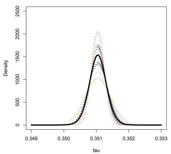
Beta-Binomial Model: Estimated density functions for the log relative risk conditional on W_i for all observed values of W across 48 studies. Thick black curve represents the marginal distribution of τ, obtained by averaging the distribution of τ_i | W_i across studies.

Under the gamma-beta framework, the estimated parameters are

$$\widehat{\alpha }=1.44,\widehat{\beta }=383.8,\log \left(\widehat{\psi }\right)=19.8,\text{and}\widehat{\gamma }=1.33.$$

The corresponding 95% confidence interval for γ is [0.96,1.84] and this approach suggests a marginally significant evidence that there is an elevated risk of MI in the treated group with a p-value of 0.085 for testing γ = 1. In Figure 3, we display the estimated density of τ_i | W_βi = ω, ${\widehat{f}}_G(\tau \mid \omega ,\widehat{\theta })$, for all the observed values of $W_{\widehat{\beta }i}$ in the rosiglitazone dataset. Averaging over all studies, we also obtained the marginal distribution of τ_i. The estimated median of the marginal distribution was 0.284 with standard error 0.164 and 95% confidence interval [−0.038, 0.61]. The p-value for testing median log relative risk being 0 is 0.087, which is consistent with the results from the normal prior. The between study heterogeneity was also very small with a standard deviation of 2.21 × 10⁻⁴ for the relative risk. Using the proposed likelihood ratio test for τ_i = 0, the p-value is 0.16.

Figure 3.

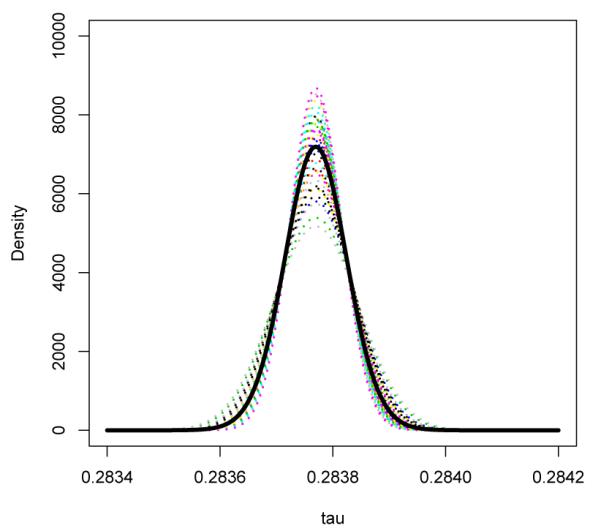
Beta-Gamma Model: Estimated density functions for the log relative risk conditional on W_βi for all observed values of W_i across 48 studies assuming that p_i ~ Beta(ψγ, ψW_βi). The thick black curve represents the marginal distribution of τ by averaging the distribution of τ_i | W_βi across studies.

To compare the model fit, we show in Table 2 the AIC and BIC for all the above four models. Note that the BIC is an approximation to the log marginal likelihood of a model, and therefore, the difference between two BIC estimates may be a good approximation to the natural log of the Bayes factor [20]. Given equal priors for all competing models, choosing the model with the smallest BIC is equivalent to selecting the model with the maximum posterior probability. The fixed relative risk model with Gamma baseline was preferred over the the random relative risks with Gamma baseline. This is expected since little between study heterogeneity was found in such cases. It is interesting to observe that the conditional model was considered the best choice for this setting. Our numerical studies (details not reported) suggest that with extremely rare events, we find that the conditional model was often preferred based on these criteria. On the other hand, when the event rate is not too low, the Gamma-Beta approach is often preferred. This is consistent with our expectation of information loss due to the conditioning when there is sufficient data to estimate the baseline event rate well. Although the information criteria selects the conditional approach for the rare event data, results from our simulation studies suggest that the estimator from the conditional approach may be unstable with large bias. Thus caution should be used when interpreting results from the conditional approach.

4.2. Simulation Studies

We conducted simulation studies to examine the performance of our proposed procedures in finite samples. Several configurations were considered. The sample sizes are generated by sampling the paired sample sizes from the rosiglitazone data. For a given pair of N_i1 and N_i2, we generated the total number of events for the two groups from

$$Y_{i2}\sim \text{Poisson}\left(N_i{\lambda }_{i2}\right),Y_{i1}\sim \text{Poisson}\left(N_i{\lambda }_{i2}{e}^{{\tau }_i}\right)\text{with}{\lambda }_{i2}\sim \text{Gamma}(1.44,\beta )$$

with β chosen to be either 380 or 38 resulting in a very rare baseline event rate of 0.38% or a moderately rare event rate of 3.8%, respectively. α = 1.44 and β = 380 were chosen to mimic the rosiglitazone study. Here, the log relative risk τ_i was generated based on τ_i = log(W_i) + logit{Beta(ψγ, ψ)} for the Beta-Binomial conditional approach and τ_i = log(W_βi) + logit{Beta(ψγ, ψ(1+β/N_i))} for the Gamma-Beta unconditional approach. Generating τ_i from these models leads to a Beta prior for p_βi = e^τi/{W_i + e^τi} and p_βi = e^τi/{W_βi+e^τi} for the two approaches. The total number of studies M was chosen to be 48 reflecting the typical number of available studies in practice and 480 reflecting the ideal situation where we expect the asymptotic results to hold. We consider ψ = 358 (log(ψ) = 5.88) and ψ = 3.58 (log(ψ) = 1.28), representing a small and large between study variation, respectively. We let γ = 1.33 which correspond to median relative risk of about 1.33 for both the Beta-Binomial model and the Gamma-Beta model. The interquartile range for the relative risk is around 0.10 when log(ψ) = 5.88 and 1.10 when log(ψ) = 1.28. The empirical biases, the sampling standard errors, and the average estimated standard errors for γ and log(ψ) are summarized in Table III. The results are based on 2000 simulated datasets. Note that the proportion studies with zero events in both arms is about 4% (about 2 out 48) when β = 38 and 34% (about 16 out of 48) when β = 380.

Table III.

Biases, sampling standard errors (SSE) and average of estimated standard errors (ASE) of $\widehat{\gamma }$ and $\log \left(\widehat{\psi }\right)$ with 50 and 500 Studies for the Beta-Binomial (BB) and Gamma-Beta (GB) approaches.

		β = 380
			γ = 1.33			log(ψ) = 5.88		γ = 1.33			log(ψ) = 1.28
		Bias	SSE	ASE	Bias	SSE	ASE	Bias	SSE	ASE	Bias	SSE	ASE
M=48	BB	.03	.27	.27	1.64	4.12	4.29	.49	.48	.47	.09	2.07	.99
	GB	.02	.27	.27	1.99	4.15	3.67	.08	.37	.33	1.68	3.61	2.04
M=480	BB	.01	.08	.08	.29	1.74	3.44	.04	.14	.14	−.49	.20	.19
	GB	.00	.08	.08	.46	2.05	3.04	.01	.10	.10	.03	.25	.25

		β = 38
		γ = 1.33			log(ψ) = 5.88			γ = 1.33			log(ψ) = 1.28
		Bias	SSE	ASE	Bias	SSE	ASE	Bias	SSE	ASE	Bias	SSE	ASE
M=48	BB	.01	.09	.09	1.52	3.51	1.66	.18	.22	.21	−.04	.31	.09
	GB	.00	.09	.09	3.60	4.48	1.39	.02	.19	.12	.07	.33	.20
M=480	BB	.00	.03	.03	0.32	1.57	1.04	.16	.07	.07	−.11	.09	.09
	GB	.00	.03	.03	1.38	3.01	1.47	.00	.06	.06	.01	.09	.09

First consider the setting when the baseline event has a very low rate of 0.38%. In the absence of substantial between study variation, both methods estimate the center parameter γ well with negligible bias and almost identical standard errors. Interestingly, this is consistent with results from the fixed effects framework. The conditional and unconditional approaches result in almost identical estimates of the relative risks. On the other hand, both methods appear to have difficulty estimating log(ψ). This is not surprising since 1/ψ, reflecting the between study variation, is close to the boundary of the parameter space. When we increase the between study variation and let log(ψ) = 1.28, the unconditional Gamma-Beta approach clearly becomes preferable to the conditional Beta-Binomial approach. The conditional approach tends to produce biased estimates even with 480 studies. For the estimation of γ with M = 48, the conditional approach results in a bias of 0.49 and mean squared error (MSE) of 0.47 whereas the unconditional approach results in a bias of 0.08 and MSE of 0.14. Thus, the unconditional approach is more than three times as efficient as the conditional approach with respect to MSE. For the estimation of log(ψ) with M = 48, the conditional approach appears to be more stable compared to the unconditional approach with much smaller bias. On the other hand, with M = 480, both approaches provide stable estimates with the unconditional approach being preferable with a smaller MSE of 0.06 compared to the MSE of 0.28 with the conditional approach.

When the baseline event has a moderately low rate of 3.8%, we observe similar patterns as described above for the case with small between study variation. Both approaches seem to be able to estimate γ and log(ψ) better compared with the rare event case. Both approaches produce stable and similar estimates for γ. The estimates for log(ψ) remain unstable when there is little between study heterogeneity. When the between study variation is larger, both approaches could estimate γ and log(ψ) well. The conditional approach continues to produce slight biases in the estimated γ. The unconditional approach yields stable estimators of γ and log(ψ) with negligible biases. When M = 480, the MSEs for (γ, log(ψ)) are (0.031, 0.020) for the conditional approach and (0.008, 0.004) for the unconditional approach. Thus, with respect to MSE, the unconditional approach is still significantly more efficient compared to the conditional approach.

Across all settings considered, the estimated standard errors are close to the sampling standard errors for γ suggesting the validity of using observed information matrix for making inference in finite sample. When there is significant between study variation, the standard error estimates for log(ψ) are also close to observed sampling standard errors. However, inference for log(ψ) appears to be unreliable when the true log(ψ) is large, i.e. when there is little between study variation.

To test the null hypothesis that there is no treatment effect, we compared our proposed likelihood ratio test to the fixed effects approach with Gamma baseline as well as to the standard approaches based on the fixed effects Mantel-Haenszel (MH) with and without 0.5 imputation for zero cells, the DerSimonian and Laird (DL) random effects which use 0.5 imputation as well as Peto’s method with fixed effects (P_F) and with random effects (P_R). For the P_R, Peto’s log odds ratio and its standard error are utilised in the random effects model. The detailed implementation of such random effects approaches can be found in [21]. For comparison, we also performed testing based on the fully Bayesian approach with prior distributions selected the same as described above. To mimic the diabetes example, we generated the data with sample sizes (N_i1, N_i2) fixed the same as in the example. For each study, we generated Y_i2 from Poisson(N_i2λ_i2) and Y_i1 from Poisson(N_i1λ_i2e^τi) with λ_i2 ~ Gamma(1.44, 380) and e^τi generated from various Gamma distributions to reflect different degree of treatment effect. For each of the configuration, we generated 2000 datasets and summarized the empirical size or power of all the tests at the type I error rate of 0.05.

We first assessed the validity of the tests in finite sample by generated the data under the null setting (a) with τ_i = 0 or e^τi = 1. As shown in Table IV, the empirical sizes of the proposed likelihood ratio tests are reasonably close to the nominal level. The conditional approach yields a size of 0.044 and the Gamma-Beta approach yields a size of 0.040 when n = 48. Similar sizes are observed for the standard methods except that both the MH and DL methods with artificial 0.5 imputations yielded inflated sizes when M = 480. This raises the concern of applying arbitrary imputations, which has been noted in existing studies [5, 6]. The empirical size of the FB approach also appears to be slightly higher than the nominal level.

Table IV.

Empirical Size/Power of the six tests, likelihood ratio for Beta-Binomial (LR_BB), likelihood ratio for Gamma-Beta (LR_GB), fixed effects Mantel Hansel with 0 imputation (${\mathrm{MH}}_{\mathrm{F}}^{\left(0\right)}$) and with 0.5 imputation (${\mathrm{MH}}_{\mathrm{F}}^{\left(0.5\right)}$), DerSimonian-Laird random effects with 0.5 imputation (${\mathrm{DL}}_{\mathrm{R}}^{\left(0.5\right)}$), Peto’s method with fixed (P_F) and random effects (P_R), fully Bayesian approach (FB), as well as the fixed (Fix) relative risk approach with Gamma baseline for three settings: (a) e^τi = 1; (b) e^τi ~ Gamma(66.5, 50); and (c) e^τi ~ Gamma(0.665, 0.5).

		LRBB	LRGB	${\mathrm{MH}}_{\mathrm{F}}^{\left(0\right)}$	${\mathrm{MH}}_{\mathrm{F}}^{\left(0.5\right)}$	${\mathrm{DL}}_{\mathrm{R}}^{\left(0.5\right)}$	PF	PR	FB	Fix
a	M = 48	.044	.040	.054	.046	.034	.056	.043	.042	.055
	M = 480	.045	.048	.051	.142	.192	.051	.047	.078	.052
b	M = 48	.254	.269	.320	.169	.093	.324	.288	.109	.338
	M = 480	.998	.998	.999	.949	.785	.998	.998	.974	.998
c	M = 48	.833	.914	.422	.355	.102	.422	.101	.233	.430
	M = 480	1.00	1.00	.875	.742	.122	.875	.076	.932	.880

To compare the power of the tests, we considered two different settings: (b) e^τi ~ Gamma(66.5, 50); and (c) e^τi ~ Gamma(0.665, 0.5). Both settings yields an average relative risk of 1.33, but the between study variability is small (std deviation = 0.16) in setting (b) and is large (std deviation = 1.63) in setting (c). With a small between study variability, testing under the fixed effects framework may be more powerful since additional parameter estimations are required in the random effects framework. This is consistent with the results shown in Table IV. All the fixed effects procedures without imputations are slightly more powerful compared to the proposed likelihood ratio tests. The MH method with 0.5 imputation appears to have much less power compared to other methods. This is likely due to the imputation of 0.5 which may result in a significant variance over-estimation for rare event settings. Furthermore, when n = 48, all the tests have rather limited power (ranging from 9.3% to 33.8%) in detecting the treatment difference. With a large between study variation in setting (c), one may fail to detect the treatment difference by only assessing the center of the relative risks. With n = 48, the fixed effects approach yield tests with 42% of power for the Peto’s method, 36% of power for MH method and 43% of power for the fixed effects approach with Gamma baseline. In the contrary, the proposed likelihood ratio tests yield 83% of power based on the conditional approach and 91% of power based on the Gamma-Beta approach. Furthermore, the standard approaches with random effects including the fully Bayesian approach have only about 10% of power in detecting the difference when the tests are only focused on the mean relative risks. This is partially due to the fact that the standard approaches focus on the testing of μ = 0 as for fixed effects models without restricting the null to be τ_i = 0 across all studies.

5. DISCUSSION

In this paper, we proposed the use of Poisson random effects model to combine 2 × 2 tables from multiple studies when the event rates for individual studies are rare. In the presence of between study heterogeneity, the mean log-relative risk can only be viewed as the center of the distribution of the treatment effect. For such settings, it is important to assess the amount of between study heterogeneity in the log-relative risk which also captures information regarding the treatment effect. The proposed likelihood ratio tests are useful tools for assessing the overall treatment effects. Simulation results suggest that the proposed tests are more powerful compared to the standard tests when there is a high level of between study variation. We took advantage of the conjugacy of the Poisson and Gamma distributions, as well as of Beta and the Binomial distributions to obtain closed-form likelihood functions. One potential drawback of the proposed approach is that the Beta prior imposed on p_i and p_βi implicitly specifies the prior of τ_i to be dependent on the relative sample size allocation. In practice, the maximum likelihood estimators may be obtained easily through standard optimization algorithms such as nlmin in R or the Newton Raphson algorithm. The R code for implementing the proposed procedures is available upon request.

The proposed procedures can be easily extended to incorporate additional covariates. The study level covariates such as treatment duration could be incorporated easily. Covariates thought to influence baseline event rates could be simply added as linear terms into the basic log-linear model (1) on λ_ij. Covariates thought to influence the relative risk itself could be incorporated as interaction effects. The methods could also be extended to analyze individual patient level data to incorporate patient level covariates such as age or gender. For such an extension, one may consider the poisson model as an approximation to the binomial model with rare events and model the covariate effect multiplicatively on the probability of experiencing an adverse event. Although a large population of studies would be needed in order to have precision to assess the impact of covariates, such a meta-regression approach would, in theory, provide a highly valuable strategy for exploring whether the treatment differences vary across sub-populations. Such explorations could be used to identify sub-populations with particularly high or low risks of adverse events. The proposed procedures could also be extended to analyze time to event data by extending the poisson model to the exponential model. Consider the simple setting without additional covariates, the likelihood contribution from the jth treatment group of the ith study is simply ${\lambda }^{{\stackrel{‒}{d}}_{ij}}{e}^{-\lambda {\stackrel{‒}{c}}_{ij}}$, where ${\stackrel{‒}{d}}_{ij}={\sum }_{k=1}^{N_{ij}}{\delta }_{ijk}$ and ${\stackrel{‒}{c}}_{ij}={\sum }_{k=1}^{N_{ij}}(1-{\delta }_{ijk})t_{ijk}$, δ_ijk is the indicator of experiencing an event during the follow up time and t_ijk is the minimum of the event time and the follow up time for the kth subject in the study. Our procedure would follow immediately by replacing the poisson likelihood with the above likelihood.

Through simulation studies, we find that the conditional approach, which essentially deletes studies with zero events in both treatment arms, may result in biased estimates when the underlying event rate is low and the between study variation is not small. However, the bias does diminish as we increase the study sample sizes and the type I error for testing γ = 1 is close to the nominal level when the study sample sizes are increased to an average level of 2000. On the other hand, the unconditional approach, which utilizes information across all studies, performs well in estimating the relative risk across all the settings considered in our numerical studies. In general, we find that the unconditional approach is more efficient than the conditional approach when there is a high level of between study variation and the two approaches have similar performances when there is little between study variation. It is worth noting that in order to estimate the between study variation well, one may require the study sample sizes and the number of studies to be large, especially if the baseline event rate is extremely low.

REFERENCES

- 1.Nissen S, Wolski K. Effect of rosiglitazone on the risk of myocardial infarction and death from cardiovascular causes. New England Journal of Medicine. 2007;356(24):2457–71. doi: 10.1056/NEJMoa072761. [DOI] [PubMed] [Google Scholar]
- 2.Normand S. Tutorial in biostatistics meta-analysis: formulating, evaluating, combining, and reporting. Statistics in Medicine. 1999;18:321–359. doi: 10.1002/(sici)1097-0258(19990215)18:3<321::aid-sim28>3.0.co;2-p. [DOI] [PubMed] [Google Scholar]
- 3.Mantel N, Haenszel W. Statistical aspects ofthe analysis ofdata from retrospective studies ofdisease. J. Nail. Cancer Inst. 1959;22:719–748. [PubMed] [Google Scholar]
- 4.Yusuf S, Peto R, Lewis J, Collins R, Sleight P. Beta blockade during and after myocardial infarction: an overview of the randomized trials. Prog Cardiovasc Dis. 1985;27(5):335–71. doi: 10.1016/s0033-0620(85)80003-7. [DOI] [PubMed] [Google Scholar]
- 5.Tian L, Cai T, Pfeffer M, Piankov N, Cremieux P-Y, Wei LJ. Exact and efficient inference procedure for meta analysis and its application to the analysis of independent 2 × 2 tables with all available data but without artificial continuity correction. Biostatistics. 2008 doi: 10.1093/biostatistics/kxn034. in press. [DOI] [PMC free article] [PubMed] [Google Scholar]
- 6.Bradburn M, Deeks J, Berlin J, Localio A. Russell. Much ado about nothing: a comparison of the performance of meta-analytical methods with rare events. STATISTICS IN MEDICINE. 2007;26(1):53. doi: 10.1002/sim.2528. [DOI] [PubMed] [Google Scholar]
- 7.DerSimonian R, Laird N. Meta-analysis in clinical trials. Controlled Clinical Trials. 1986;7:177–188. doi: 10.1016/0197-2456(86)90046-2. [DOI] [PubMed] [Google Scholar]
- 8.Brumback B, Cook R, Ryan L. A meta-analysis of case-control and cohort studies with interval-censored exposure data: application to chorionic villus sampling. Biostatistics. 2000;1(2):203–217. doi: 10.1093/biostatistics/1.2.203. [DOI] [PubMed] [Google Scholar]
- 9.Gatsonis C, Daniels M. Hierarchical Generalized Linear Models in the Analysis of Variations in Health Care Utilization. Journal of the American Statistical Association. 1999;94(445):29–30. [Google Scholar]
- 10.Breslow N, Clayton D. Approximate inference in generalized linear mixed models. Journal of the American Statistical Association. 1993;88(421):9–25. [Google Scholar]
- 11.Carlin B, Louis T. Bayes and empirical Bayes methods for data analysis. Statistics and Computing. 1997;7(2):153–154. [Google Scholar]
- 12.Hadjicostas P, Berry S. Improper and proper posteriors with improper priors in a Poisson-gamma hierarchical model. Test. 1999;8(1):147–166. [Google Scholar]
- 13.Lee Y, Nelder J. Hierarchical generalised linear models: A synthesis of generalised linear models, random-effect models and structured dispersions. Biometrika. 2001;88(4):987–1006. [Google Scholar]
- 14.Lord D. Modeling motor vehicle crashes using Poisson-gamma models: Examining the effects of low sample mean values and small sample size on the estimation of the fixed dispersion parameter. Accident Analysis and Prevention. 2006;38(4):751–766. doi: 10.1016/j.aap.2006.02.001. [DOI] [PubMed] [Google Scholar]
- 15.Liu J. Monte Carlo strategies in scientific computing. Springer; 2001. [Google Scholar]
- 16.Cox D, Hinkley D. Theoretical Statistics. Chapman & Hall/CRC; 1974. [Google Scholar]
- 17.Williams DA. The analysis of binary responses from toxicological experiments involving reproduction and teratogenicity. Biometrics. 1975;31:949–952. [PubMed] [Google Scholar]
- 18.Barndor-Nielsen O, Cox D. Bartlett adjustments to the likelihood ratio statistic and the distribution of the maximum likelihood estimator. J. Roy. Statist. Soc. Ser. B. 1984;46:483–495. [Google Scholar]
- 19.Murphy S, Der Vaart A. On Profile Likelihood. Journal of the American Statistical Association. 2000;95(450) [Google Scholar]
- 20.Kass R, Wasserman L. A reference Bayesian test for nested hypotheses and its relationship to the Schwarz criterion. Journal of the American Statistical Association. 1995:928–934. [Google Scholar]
- 21.StataCorp, L. Stata statistical software: Release 10. Stata Corporation; College Station, TX: 2007. [Google Scholar]