Analyzing shotgun proteomic data with PatternLab for proteomics

Abstract

PatternLab for proteomics is a one-stop-shop computational environment for analyzing shotgun proteomic data. Its modules provide means to pinpoint proteins / peptides that are differentially expressed, those that are unique to a state, and can also cluster the ones that share similar expression profiles in time-course experiments as well as help in interpreting results according to Gene Ontology. PatternLab is user-friendly, simple, and provides a graphical user interface.

Introduction

Shotgun proteomics is a powerful approach for analyzing complex peptide mixtures. The overall strategy comprises the digestion of proteins followed by peptide separation, fragmentation, and protein identification (Washburn et al. 2002). Tandem mass spectra are acquired to enable protein identification, which is commonly achieved by comparing experimental with theoretically generated spectra and pinpointing the most likely match via search engines such as SEQUEST (Eng et al. 1994), ProLuCID (Xu et al. 2006), or Mascot (Perkins et al. 1999). The identifications are then filtered according to quality scores and a false-discovery rate is estimated. SEQUEST or ProLuCID followed by DTASelect (Cociorva et al. 2007) are the search engines and filtering program, respectively, used in the protocols listed herein.

Proteins are quantitated according to label-free or label-based (e.g., SILAC (Ong et al. 2002)) strategies. For example, spectral counting is a label-free method that works with the numbers of identified spectra matched to a protein (Liu et al. 2004); it is simple and has been shown to be successful on controlled experiments with spiked proteins (Carvalho et al. 2008b). Label-based strategies yield higher confidence for relative quantitation; nevertheless, they are more expensive and laborious. The latter are performed by comparing a peptide to an internal, chemically identical standard enriched with a heavy stable isotope; the ratios informing relative abundance are then obtained computationally with a program such as Census (Park et al. 2008).

In general, protein identification and quantitation constitute the tip of the iceberg for analyzing shotgun proteomic data. Questions such as “Which proteins are differentially expressed?”, “Which are unique to a state?”, “Which share similar expression profiles in a time-course experiment?”, and even more specific questions, such as, “Which proteins originate from the mitochondria?” are all very common. PatternLab for proteomics (Carvalho et al. 2008a) is a one-stop shop for answering these types of question. PatternLab provides tools for analyzing shotgun proteomic data quantitated by spectral counting (output from DTASelect) or by the label-based (output from Census). Its modules provide means to pinpoint differentially expressed proteins / peptides (TFold / ACFold modules), pinpoint proteins that are unique to a state (Approximately area-proportional Venn diagram module), find proteins that share similar expression profiles in time-course experiments (TrendQuest module), and help interpreting results according to Gene Ontology (Gene Ontology Explorer module) (Ashburner et al. 2000; Carvalho et al. 2009). PatternLab is freely available for download at http://pcarvalho.com/patternlab or at http://fields.scripps.edu once the user has agreed to the online license provided by The Scripps Research Institute.

Necessary resources

Hardware

• A computer capable of running Windows XP with Service Pack 2 or later, VISTA, or Windows 7. A computer with a minimum of 2GB RAM and 2 or more computing cores is recommended.

Software

• Windows XP with Service Pack 2 (or later), Windows Vista, or Windows 7.

• PatternLab for proteomics, which can be freely downloaded and installed with a single click of the mouse from the project's website.

• The .NET framework 3.5, which can be automatically and freely updated by PatternLab during installation if necessary.

Files

• For relative quantitation by spectral counting: the DTASelect-filtered.txt files.

• For quantitation by labeling: the Census out.txt files.

Basic protocol 1: Parsing experimental data into PatternLab's data format

Before analyzing any results, experimental data must be parsed into PatternLab's data format (index and sparse matrix). This protocol describes how this is accomplished. It assumes that the user is comparing two biological states and has performed three replicate assays for each state; for example, let these states be named healthy and disease. PatternLab requires each state to be represented as an integer, henceforth -1 for health and 1 for disease. In all, there are 6 assays: -1A, -1B, -1C (acquired from the health state), and 1A, 1B, 1C (acquired from the disease state). The approach described by this protocol is for DTASelect (spectral counting) data; a slight modification for analyzing labeled (Census) data is described in Comments.

Steps

1. Create two directories, one named -1, the other named 1. The directory names must be integers.

2. Rename each DTASelect-filtered.txt file to the designated name such as -1A, -1B, etc.

3. Copy the renamed DTASelect-filtered.txt files to the directory corresponding to their respective states (-1 or 1).

4. Load PatternLab for proteomics and select “Parse”, followed by “DTASelect to Sparse Matrix” from the tool bar. The main screen should now change and the DTASelect parser should be displayed as in Figure 1.

5. For each directory containing the experimental results, click on the “Add a directory” button, navigate to the corresponding directory and add it to the parsing list. These controls are available in the group box entitled “Step 1: Add the directories to be parsed”.

   The Census output, in general terms, consists of intensity ratios of both labeled and unlabeled peptides; thus, a single Census output file encompasses two classes. From the PatternLab parsing perspective, only one directory should be created (-1) and the Census files placed in it. The index.txt and sparseMatrix.txt files can be generated by selecting the “Census to Sparse Matrix” option from the “Parse” drop-down menu in PatternLab's main interface. The rest is performed as described below.

6. By now, the group box entitled “Step 2: Parsing configuration” should be enabled. The user should choose between the peptide and protein radio buttons to specify if the analysis will search for differentially expressed peptides or proteins.

7. In shotgun proteomic experiments, it is common to identify peptides that share a common sequence and therefore the search engine becomes unable to pinpoint from which protein they derived. If the “combine isoforms” checkbox is selected, PatternLab will group these proteins by isoform peptides and count them as a single protein identification.

8. Finally, “Step 3” is where the user specifies the output (the index and sparse matrix files). We recommend saving these files one level above the data directories. For example, if the data directories are c:\myExperiment\-1 and c:\myExperiment\1, a good place to save the sparseMatrix.txt and index.txt files is c:\myExperiment.

9. Once this has been accomplished, press the “Parse and save project data” button.

10. For each state (directory) included, PatternLab will pop-up a window that requires the user to enter a brief description of the state. In the present example, appropriate descriptions would be “Health”, for the -1 state, and “Disease”, for the 1 state.

11. The parsed files should now have been generated and be available in the directory specified by the user.

Figure 1. The DTASelect parser.

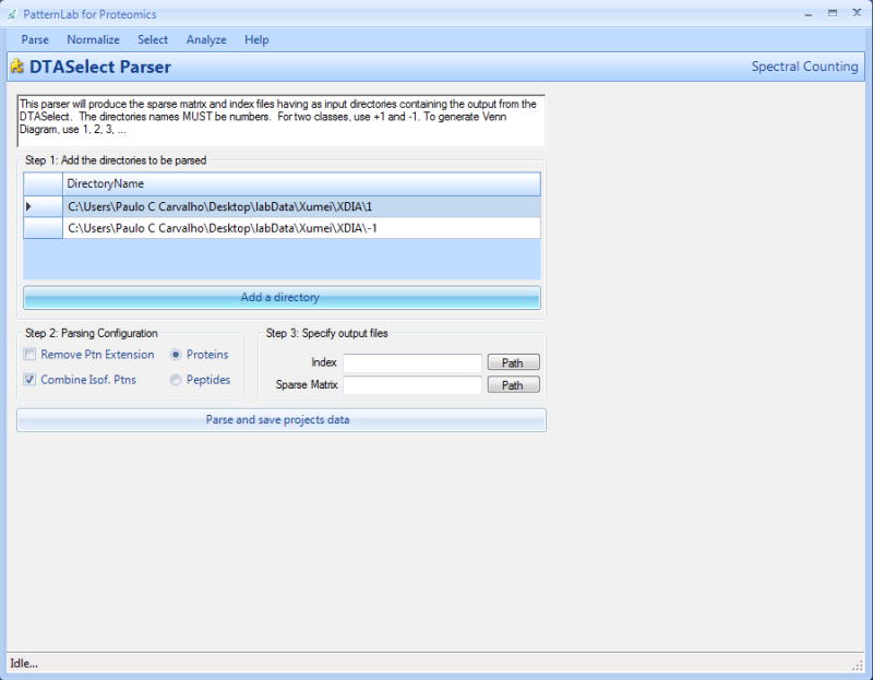
This graphical user interface is used to convert spectral counting data obtained from DTASelect into PatternLab's data format (the index and sparse matrix files).

Basic protocol 2: TFold and ACFold—Pinpointing differentially expressed proteins

Introduction

Pinpointing differentially expressed proteins in shotgun proteomics experiments is a tricky task because it deals with a massive hypothesis testing problem. PatternLab introduces the TFold and ACFold tests, which combine fold-change cutoffs with a statistical test and the Benjamin-Hochberg (BH) theoretical false-positive rate estimator (Benjamini, Hochberg 1995) to deal with the task at hand. ACFold is specific for when there is only one assay for each state and is recommended to obtain preliminary insights into the data. When more replicates are acquired for each state, then TFold is to be applied. The protocol below describes a TFold analysis.

Steps for performing a pairwise comparison

1. Load PatternLab for proteomics and choose “Select” from the main pull-down menu, followed by “TFold”. The TFold graphical user interface should load as in Figure 2.

2. Indicate the path for the sparseMatrix.txt and index.txt files generated using protocol 1 by clicking on the corresponding “Browse” button and navigating to the files.

3. Choose a normalization strategy among those available as radio buttons within the “Data normalization and fold change calculation” group box. If the analysis comprises labeled data, the “I am using labeled data” option must be chosen. In case of the latter, the option “Expected fold for single class sparse matrix” will be enabled. Further details regarding this option and other normalization strategies are provided in the Comments section.

4. The “Minimum readings (all classes summed)” feature should now be specified. This is a quality filter that works as follows; suppose for example that the user has two states (biological conditions to be compared), each having three replicates. If the “Minimum readings (all classes summed)” feature is set to 4, only proteins that appear in at least four out of all six assays (including both classes) will be considered in the analysis. This feature's default value is 2, so a protein must be found in at least two replicates. Note that in the example provided, by setting this parameter to 4 only proteins detected in both classes will be considered.

5. Press the “Parse” button; this should enable the “Parameter selection” group box. Note that if any modifications have been made heretofore to the values of the controls within the “Load matrix” group box, they will only become effective if the “Parse” button is pressed again.

6. If the sparseMatrix.txt file contains more than two classes, a pop-up will appear to query if one wishes to perform a pairwise or multi-class analysis. This protocol describes a pairwise comparison. A second pop-up (Figure 3) should then appear; it lists all available classes in the sparse matrix so the user can select which two classes to compare.

7. Press the “Calculate and plot” button. A scatter plot similar to the one in the right panel of Figure 2 should be generated. Refer to Figure 2's legend for graph interpretation.

8. Further information on each protein's dot representation can be accessed by hovering the mouse over the dot in the plot.

9. The plot's x-axis and y-axis can be re-scaled by changing the values in “Upper fold y-scale” and in “pValueLowerClip”.

10. The p-value, fold-change cutoff, and BH theoretical false-discovery rate threshold (Benjamini, Hochberg 1995) can be modified using the controls in the “Parameter selection” group box.

11. The plot and a report of the differentially expressed proteins can be saved by clicking on the “Output” tab and then on the “Save plot” and “Save flexible report” buttons, respectively. In the case of the latter, one can select the class of dots (green, red, blue, or orange) to be included in the report. Special constraints can be specified for orange (proteins that did not meet the specified fold-change cutoff but are statistically significant) and green (proteins that are not statistically differentially expressed but have a fold change greater than the specified cutoff). For example, one may wish to retain orange dots that have an exceptionally low p-value (e.g., < 0.0005) or a very high fold change (e.g., 5) for further analysis.

12. PatternLab allows the easy querying of the data by clicking on the “Scoring results” tab. In this section, a dynamically sortable table according to matrix index, fold change, p-value, protein id, quantitation information for each class, and description, is presented. The user can further query the table by inputting wild card searches in the “RegEx” query box.

Figure 2. A TFold pairwise analysis of two biological states.

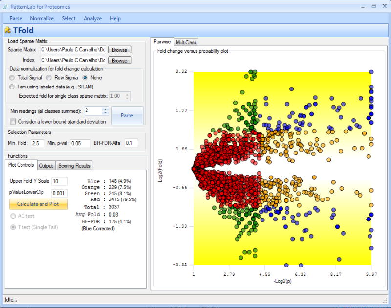
Each protein (represented as a dot) is mapped according to its log₂ (fold change) on the ordinate axis and its -log₂(t-test p-value) on the abscissa axis. The latter indicates how likely the observed fold change is a result of chance. Fold changes refer to the ratios of the average relative quantitation values obtained for each state. Accordingly, blue-dot proteins have p-value < 0.05 and an absolute fold change greater than 2.5, the established fold-change cutoff. Orange-dot proteins did not meet the fold-change cutoff but were indicated as statistically different. Green-dot proteins met the fold-change cutoff but cannot be claimed to be statistically different. Red dots did not satisfy the fold-change or the statistical cutoffs. The theoretical false-positive estimator indicates that 125 out of the 148 proteins selected as differentially expressed are likely to be truly differentially expressed.

Figure 3. Class selection pop-up.

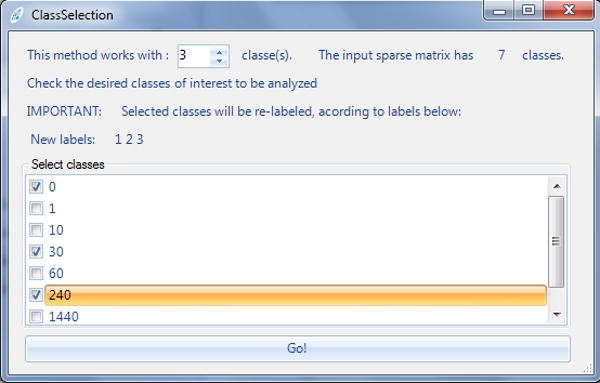
When a PatternLab module is set to analyze a sparse matrix containing more than two classes, this pop-up is displayed so the user can choose which classes to be included in the analysis. The example provided shows a sparse matrix containing seven classes.

Performing a multi-class comparison (a sparseMatrix.txt file with three or more classes)

The XFold module extends the TFold and ACFold modules to enable the analysis of multiple conditions. TFold and ACFold were originally designed for pairwise comparisons and unify a statistical test (the t-test or the AC-test, respectively) with protein expression fold changes and a theoretical false-discovery rate estimator, the latter being necessary to address the massive multiple hypothesis testing problem. The XFold algorithm proceeds as follows. First, it automatically performs a TFold (or ACFold) analysis for all component-state pairs. Secondly, a table is generated with a row for each identification (id) and a column for each state. A table entry indicates, as 1 (differentially expressed) or 0 (not differentially expressed), the result of the analysis for the corresponding id's in the corresponding state. Thirdly, a score is obtained by computing how many times a protein was classified as differentially expressed (i.e., summing up each row's entries). Finally, the table's rows are sorted by score and then can be clustered according to the Hamming distance between consecutive rows. This results in groups of components (rows) that were differentially expressed for roughly the same set of different conditions.

We note that, while typical shotgun proteomic assays identify and quantify thousands of proteins, many are quantitated near, or even below, the lower bound of the method's dynamic range. Moreover, estimates of a protein's quantitation variance, especially in these borderline cases, are further impacted by the limited number of replicate analyses (usually three). By directly applying a statistical approach without taking the necessary precautions that are inherent to the XFold analysis, many marginal cases that are likely to be an artifact of chance can be included in the results and shadow important aspects.

Steps

1. Perform steps 1-4 as described above for pairwise comparisons.

2. A second pop-up should appear querying the user with the following: “Is this a pairwise comparison?”; the user should click on the “No” button.

3. The “Parameter selection” group box options should then be handled as described above for pairwise comparisons.

4. Click on the “Calculate and plot” button. The “Multi-class” tab should automatically be selected on the right panel and a result table should appear as shown in Figure 4.

5. Clicking on the “Cluster by Hamming distance” button is recommended to sort rows (id's) that were differentially expressed for roughly the same set of different conditions.

Figure 4. The XFold graphical user interface.

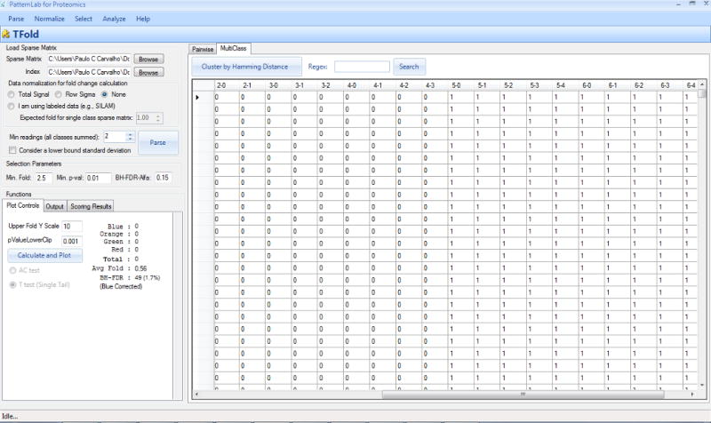
XFold is used when pinpointing differentially expressed proteins in a multi-class analysis.

Basic Protocol 3: AAPVD—Approximately area-proportional Venn diagram

The AAPVD module complements the TFold and ACFold strategies by pinpointing proteins that are unique to a state. It is also useful to assess the quality of technical replicates. By double-clicking on each legend (numbers within the circles) in the Venn diagram (Figure 5), a list of the unique id's and further details (e.g., spectral counts, etc.) are provided. When analyzing more than two conditions simultaneously, a table listing the unique components of every pairwise combination of conditions is also provided. By clicking on the table entry of interest, the unique id's are listed.

Figure 5. The AAPVD graphical user interface.

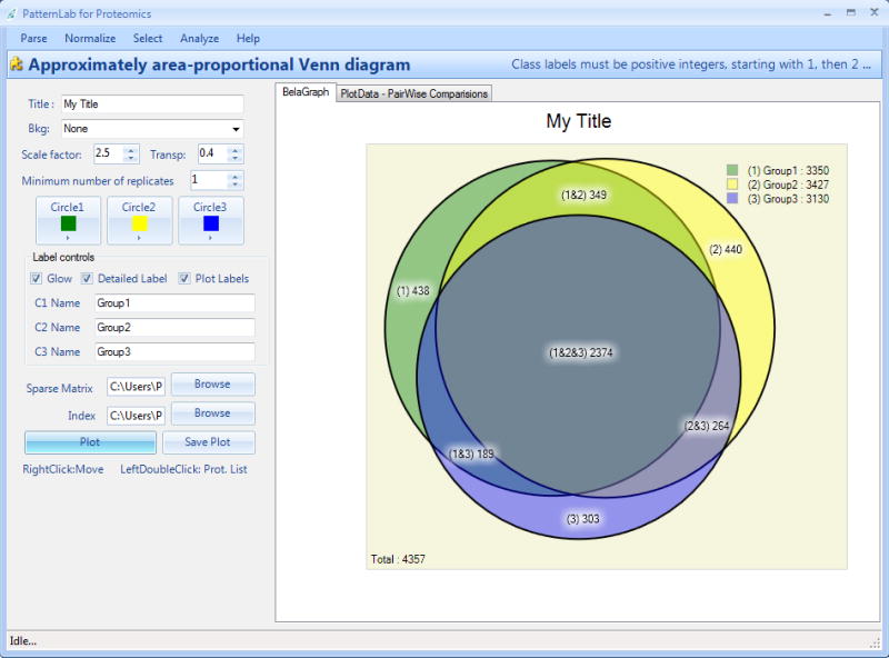
This tool's main usage is to pinpoint unique proteins to a state and to obtain a bird's eye view of how different the states are.

Steps

1. Load PatternLab for proteomics and select “Analyze”, followed by “Approximately area-proportional Venn diagram (AAPVD)”. The AAPVD graphical user interface should load as in Figure 5.

2. Indicate the path for the sparseMatrix.txt and index.txt files by clicking on the corresponding “Browse” button and navigating to the files.

3. If the sparseMatrix.txt file has three or more classes, a “Class selection” pop-up window (Figure 3) will appear for selecting the classes to include in the analysis. In the example provided in Figure 5, sparseMatrix.txt has seven classes and the user is selecting three classes.

4. (Optional step) Type a title for the plot, select a background color / image using the “Bkg” pull-down menu, and choose colors for the Venn diagram circles.

5. Specify a value for the quality filter “Minimum number of replicates”. For example, by selecting 2, only biomolecules found in at least two replicates of each class will be considered.

6. By clicking on the “Plot” button, the Venn diagram should be plotted.

7. The positioning of the labels is inferred automatically; therefore they should be double-checked. In case one wishes to change the position of a label, this can be done by right-clicking on it and dragging it to the desired position.

8. The biomolecules referred to in a certain part of the Venn diagram can be discriminated by double-clicking on the respective label. For example, if one wishes to know what are the 438 proteins that are unique to group 1 in figure 5, this information can be made available by double-left-clicking on the respective label. Moreover, the table will contain information such as the protein index from the index.txt file, the protein's name, the number of replicates it was detected in, the sum of its signal intensities, spectral counts, and the protein's description. This report can be exported by clicking on the “Save” button in the topmost part of the window.

9. The Venn diagram circles can be made larger or smaller by modifying the value in the “Scale factor” control.

10. Pairwise comparisons between all classes contained in the analysis can be accessed by clicking the “Plot data – pairwise comparisons” button.

Basic protocol 4: TrendQuest

The TrendQuest module clusters components with similar expression profiles according to the hierarchical or k-means clustering algorithms. Its graphical user interface is shown in Figure 6. This module provides various custom data filters tailored to the specificities of shotgun proteomics, such as discarding proteins averaging below a certain spectral count threshold or proteins that were not detected within a certain number of replicate experiments. Options such as normalizing according to internal standards or total spectral counts / total signal are also provided. The cluster profiles are displayed in the graphical user interface and descriptive information on each element is available when hovering the mouse over a specific trend line.

Figure 6. The TrendQuest graphical user interface.

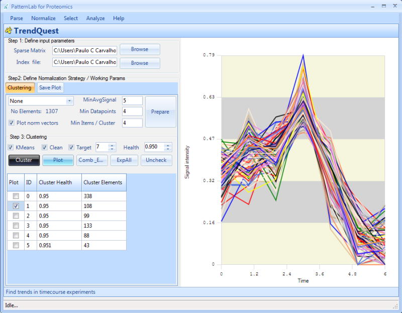
This tool is used to group proteins / peptides that have similar expression profiles.

Steps

1. Load PatternLab for proteomics and select “Analyze”, followed by “TrendQuest”; its graphical user interface should appear as in Figure 6.

2. Indicate the path for the sparseMatrix.txt and index.txt files by clicking on the corresponding “Browse” button and navigating to the files.

3. Choose a normalization strategy from the pull-down menu located in the “Step 2” group box.

4. The quality filters should now be set. The “MinAvgSignal” filter will establish a cutoff to eliminate proteins / peptides whose spectral counts, for example, fall below a desired value. The “Min data points” filter establishes a cutoff for eliminating identifications that do not appear within a minimum number of assays. The “Min items / cluster” filter will eliminate clusters containing fewer elements than the amount specified.

5. Click on the “Parse” button; this should unlock the “Step 3: clustering” group box.

6. By pressing the “Cluster” button, TrendQuest performs hierarchical clustering using the Pearson correlation coefficient as a distance measure. The results should be made available in the table below.

7. Alternative to step 6: Click on the “k-means” checkbox to have this algorithm used instead. It will target the number of clusters specified in the “Target” numeric control. A final filtering step is performed that removes elements from any cluster whose Pearson correlation coefficient falls below the value specified in the “Health” numeric control. The Pearson correlation coefficient is computed by comparing the trend of an element in the cluster against a global trend obtained by averaging all elements from the cluster.

   TrendQuest offers two algorithms for clustering data: hierarchical clustering (HC), which is the default, and k-means. HC yields reproducible results; clustering will be carried on while there are at least two clusters that can be coalesced to produce a new cluster for which the Pearson correlation coefficient of each cluster member to a cluster representative (average of all cluster members) is higher than the cutoff specified by the user. The k-means clustering method is expected to produce results similar to those of HC, but it is not reproducible. On the other hand, it allows one to specify the number of desired clusters. PatternLab carries out the k-means algorithm 100 times and outputs the best solution (the one that maximizes inter-cluster distances). Typical values for the Pearson correlation coefficient cutoff are 0.9 and 0.95.

8. A table listing the available clusters and the number of elements in each one is presented when the clustering process is finished. By selecting the checkbox besides each cluster and clicking on the “Plot” button, a plot of the trend in the cluster is generated as exemplified in Figure 6.

9. By hovering the mouse over each trend line, a pop-up is displayed that indicates the protein / peptide from which the respective trend line originates.

10. A list of the proteins contained in each of the trends whose checkboxes were selected can be exported to text files using the “ExpAll (export all)” button.

11. Trends can be combined by selecting simultaneously more than one of the trend checkboxes. They can be jointly exported to text files by clicking on the “Combine_export” button.

12. When the “Plot norm vectors” checkbox is selected, each trend will be normalized to have a norm (L2-norm) equal to 1.

GOEx—Gene Ontology Explorer

GOEx leverages the gene ontology (GO) (Ashburner et al. 2000) to aid in the interpretation of proteomic data. It can be used to interpret lists of protein id's or the output from TFold / ACFold directly. GOEx stands out because it can combine data from protein fold changes with GO over-representation statistics to help draw conclusions. Moreover, it is tightly integrated into the PatternLab for proteomics project and, thus, lies within a complete computational environment that provides parsers and pattern recognition tools designed for spectral counting or analyzing labeled data.

Basic protocol 5: Compiling the latest GO and gene ontology annotation (GOA) into GOEx's pre-computed format

Any analysis performed by GOEx requires the GO OBO database and the GOA association file containing the non-redundant, species-specific annotations. This protocol describes how to obtain these files and have GOEx merge them with various pre-computations (e.g., mapping all terms descending from a specific term) to speed up the user's experience when analyzing data. The final output will be a file having the extension .precomp (pre-computed) and should be used in future GOEx analyses.

Steps

1. Load PatternLab for proteomics and select “Analyze”, followed by “GOEx”; its graphical user interface should appear as in Figure 7.

2. Download the latest GO OBO v1.2 file. To accomplish this, first click on the “?” link on the right-hand side of the “Load GO DAG” button.

3. A browser should automatically open with the appropriate GO address. The latest GO OBO file can be downloaded by right-clicking on the appropriate link and selecting “Save as”.

4. The species-specific GOA should be downloaded similarly by clicking on the “?” link located on the right-hand side of the “Load associations” button. Usually, this file requires decompression.

5. Click on the “Load GO DAG” button and select the GO OBO file. PatternLab should perform some optimizations, so this process is expected to take about one minute.

6. Click on the “Load associations” button and load the respective file. This should enable the “SavePreComp” button.

7. Save the pre-computed file by clicking on the “SavePreComp” button. It should take about 10 seconds to generate the file.

8. Step 6 should also unlock the lower panel, with the GO roots appearing in the “iDAG viewer”.

9. For future usage, one can now load the .precomp file instead of separately loading the GO and GOA files. This can be performed by clicking on the “Load precomp” button.

Figure 7. The GOEx graphical user interface.

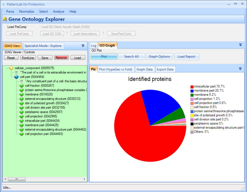
GOEx leverages GO to aid in the interpretation of shotgun proteomic data. It can also consider expression fold changes.

Analyzing data with GOEx

GOEx makes available three orthogonal strategies for analyzing data. They are the iDAG (interactive directed acyclic graph), the specialist mode, and the over-representation automatic search. These strategies correspond to modules, which take as input the report of differentially expressed proteins provided by TFold or ACFold or, alternatively, a list of proteins following PatternLab's index file format. Recall that the latter comprises three columns, the first containing a unique integer, the second a protein identifier (e.g., IPI), and the third the protein's description. Note that when using protein lists information on fold change is not available and therefore GOEx cannot take advantage of this information in the analysis. The usage of the three GOEx modules is described below.

iDAG

The iDAG tool is located in the lower green panel (Figure 7). Initially, it displays the three GO root terms. This strategy is designed to help guide one's biological questions by leveraging the GO through the iDAG, coupled with graphing tools. By clicking on an iDAG term, its child terms appear listed below it. Terms having no relation to the reported proteins are automatically deleted to keep the biological questions on track. A distribution pie chart (Figure 7) of the number of proteins mapped to each iDAG leaf terms is presented and updated every time the “Plot” button is clicked. A report table discriminating all calculations (e.g., hypergeometric p-value, group fold change, and others) is also made available. This table can be accessed by clicking on the “Graph data” tab. All this information can aid in choosing which term to explore next, thus helping drive one's biological questions. In general, terms having low p-values and/or high-magnitude fold changes are good candidates. Usually, existing GO tools tend to overlook fold changes and are limited to reporting over-represented p-value terms exclusively (Carvalho et al. 2009).

The specialist mode

The specialist mode can be accessed by clicking on the “Specialist mode” tab and then entering a wild card search. For example, entering “mitoch” will search for GO terms that match “mitochondria”, “mitochondrial”, etc. and are related to the provided list of proteins. This mode allows an expert to pose questions and retrieve answers in the light of the GO and the reported proteins. Terms related to the reported proteins (either through fold change or over-representation) are then analyzed, plotted, and added to the report table.

The over-representation automatic search

The automatic mode (search all) performs an extensive analysis by searching for relations between the reported proteins and each and every GO term. This module requires the user to specify the desired minimum number of proteins related to a GO term, a minimum GO depth, an over-representation p-value, and optionally, a false-discovery rate (Benjamini, Hochberg 1995) cutoff. We define GO depth as the length of the shortest path from a term to its root. GOEx then evaluates all GO terms, and the ones bearing relation to the reported proteins will be listed in the report table and plotted in the distribution pie chart.

Guidelines for understanding results

1. TFold and ACFold

1.1 Taking advantage of the false-discovery rate estimator

The aim of the BH false-discovery rate (BH-FDR) is to help in choosing cutoff parameters. For example, note that 148 proteins are represented by blue dots, or differentially expressed, in Figure 2; however, the BH-FDR estimator points out that for only 125 of them this is likely to be true. In the ideal case, these numbers should match; however, the BH-FDR is known to be conservative, which makes the result acceptable. By raising the fold-change cutoff, fewer proteins will be classified as blue-dot ones, thus lowering the difference between the number given by the theoretical estimator and that of the proteins statistically selected as differentially expressed. Another alternative is to use a lower p-value.

In all, the BH-FDR should be used as a guide to help with the tuning of the parameters. For example, if the same dataset is analyzed for a fold-change cutoff equal to 1, then 372 proteins are reported as differentially expressed; however, the BH-FDR indicates that only 112 of them are really likely to be differentially expressed. As can be noticed, the software suggests that changes should be made to the selection parameters in order to make the selection more stringent. The number of estimated differentially expressed proteins provided by the false-discovery estimator was indeed very similar to the ones used when obtaining the results described.

1.2 Analyzing labeled data

Labeled data provided by Census originates from ratios of intensities obtained from labeled and the analogous unlabeled peptides. PatternLab uses the one-sample t-test to compute a probability of change in expression under the premise that there should be no fold change (expected fold change of 1). Moreover, PatternLab allows the user to change the value of the expected fold change using the “Expected fold for single class sparse matrix” control located in the “Load sparse matrix” group box. This is recommended when the average fold change obtained from all molecules analyzed deviates far (> 0.1) from 1. Note that the global average fold change is reported in the result table, and that the data must be parsed again if any modifications are made to controls located in this group box.

2. GOEx

All GOEx query methods provide a complementary report table that can be dynamically sorted according to convenience. The table headers include: “GO ID”, “Term name”, “Namespace”, “Absolute fold change”, “Fold change”, “HypeGeo p”, “Study set”, “Population”, “Identified in study set”, “Identified in population”, “Protein IPI's and folds”, “GO depth”, and “Description”. “GO ID” and “Term name” specify the unique GO identifier and its name as given in the GO. “Namespace” points to which GO name space the selected term belongs to (molecular function, cellular component, or biological process). “Absolute fold change” is the sum of the absolute values of the fold changes of all proteins mapped onto a given GO term. Similarly, “Fold change” is the sum all their fold-change values. Current GO tools usually do not report on fold-change information. “HypeGeo p” is an abbreviation for the term's over-representation p-value. “Study set” refers to all the terms that descend from a given term. “Population” stands for all the terms contained within the specified term's name space. The two “Identified” headers refer to how many of the proteins discriminated in the input data were mapped onto the specified term. “Protein IPI's and folds” discriminates all the proteins, and respective fold changes, mapped onto the selected term. Finally, “GO depth” and “Description” refer, respectively, to the term's GO depth and description.

Commentary

Background information

PatternLab is a simple to use, yet efficient and panoptic software to address various typical challenges posed by shotgun proteomic data analysis. These challenges encompass pinpointing differentially expressed proteins (TFold and ACFold modules), identifying proteins that are unique to a state (AAPVD module), grouping proteins that share similar expression profiles across time course experiments (TrendQuest module), and understanding biological data according to GO (GOEx module). We are permanently committed to including new modules (as can be seen in the literature, the three latter modules were not part of the first release). PatternLab includes an automatic update feature that ensures the user will always have the latest version, but with the option to roll back and return to the previously installed version.

Critical parameters

TFold and ACFold

The results from a TFold / ACFold analysis are summarized in a table contained within the “Plot control” tab. The table discriminates the number of blue, green, orange, and red dots (proteins or peptides). Usually, the user is interested in exporting the blue-dot proteins as well as the orange–dot proteins that achieve an exceptionally low p-value. A common question to ask is “What fold-change cutoff should I use?” or “What p-value cutoff is good?”. Typical values used when analyzing spectral counting data are a 2.5 fold-change cutoff, and p-values of 0.05 and 0.01 for the TFold and ACFold analyses, respectively. For labeled data (we recall that only TFold can be applied to labeled data), the recommended values are a minimum of 1.5 and 0.05 for the fold change and the p-value, respectively. A typical BH-FDR value is 0.1; this is because of the conservative nature of the test.

AAPVD

A typical value for the quality filter “Minimum number of replicates” is 2. This will make the algorithm consider only biomolecules found in at least two replicates of each class.

TrendQuest

A typical value for the Pearson correlation coefficient used for clustering is 0.95.

GOEx

A typical p-value for the automatic search is 0.01. The BH-FDR value is typically 0.05.

Literature Cited

- Ashburner M, Ball CA, Blake JA, Botstein D, Butler H, Cherry JM, Davis AP, Dolinski K, Dwight SS, Eppig JT, Harris MA, Hill DP, Issel-Tarver L, Kasarskis A, Lewis S, Matese JC, Richardson JE, Ringwald M, Rubin GM, Sherlock G. Gene ontology: tool for the unification of biology. The Gene Ontology Consortium Nat Genet. 2000b;25:25–29. doi: 10.1038/75556. [DOI] [PMC free article] [PubMed] [Google Scholar]
- Benjamini Y, Hochberg Y. Controlling the false discovery rate: a practical and powerful approach to multiple testing. J R Stat Soc Ser B. 1995;57:289–300. [Google Scholar]
- Carvalho PC, Fischer JS, Chen EI, Domont GB, Carvalho MG, Degrave WM, Yates JR, III, Barbosa VC. GO Explorer: A gene-ontology tool to aid in the interpretation of shotgun proteomics data. Proteome Sci. 2009;7:6. doi: 10.1186/1477-5956-7-6. [DOI] [PMC free article] [PubMed] [Google Scholar]
- Carvalho PC, Fischer JS, Chen EI, Yates JR, III, Barbosa VC. PatternLab for proteomics: a tool for differential shotgun proteomics. BMC Bioinformatics. 2008a;9:316. doi: 10.1186/1471-2105-9-316. [DOI] [PMC free article] [PubMed] [Google Scholar]
- Carvalho PC, Hewel J, Barbosa VC, Yates JR., III Identifying differences in protein expression levels by spectral counting and feature selection. Genet Mol Res. 2008b;7:342–356. doi: 10.4238/vol7-2gmr426. [DOI] [PMC free article] [PubMed] [Google Scholar]
- Cociorva D, Tabb L, Yates JR. Validation of tandem mass spectrometry database search results using DTASelect. Curr Protoc Bioinformatics. 2007;Chapter 13 doi: 10.1002/0471250953.bi1304s16. Unit. [DOI] [PubMed] [Google Scholar]
- Eng JK, McCormack L, Yates A, Yates JR., III An Approach to Correlate Tandem Mass Spectral Data of Peptides with Amino Acid Sequences in a Protein Database. J Am Soc Mass Spectrom. 1994;5:976–989. doi: 10.1016/1044-0305(94)80016-2. [DOI] [PubMed] [Google Scholar]
- Liu H, Sadygov RG, Yates JR., III A model for random sampling and estimation of relative protein abundance in shotgun proteomics. Anal Chem. 2004;76:4193–4201. doi: 10.1021/ac0498563. [DOI] [PubMed] [Google Scholar]
- Ong SE, Blagoev B, Kratchmarova I, Kristensen DB, Steen H, Pandey A, Mann M. Stable isotope labeling by amino acids in cell culture, SILAC, as a simple and accurate approach to expression proteomics. Mol Cell Proteomics. 2002;1:376–386. doi: 10.1074/mcp.m200025-mcp200. [DOI] [PubMed] [Google Scholar]
- Park SK, Venable JD, Xu T, Yates JR., III A quantitative analysis software tool for mass spectrometry-based proteomics. Nat Methods. 2008;5:319–322. doi: 10.1038/nmeth.1195. [DOI] [PMC free article] [PubMed] [Google Scholar]
- Perkins DN, Pappin DJ, Creasy DM, Cottrell JS. Probability-based protein identification by searching sequence databases using mass spectrometry data. Electrophoresis. 1999;20:3551–3567. doi: 10.1002/(SICI)1522-2683(19991201)20:18<3551::AID-ELPS3551>3.0.CO;2-2. [DOI] [PubMed] [Google Scholar]
- Washburn MP, Ulaszek R, Deciu C, Schieltz DM, Yates JR., III Analysis of quantitative proteomic data generated via multidimensional protein identification technology. Anal Chem. 2002;74:1650–1657. doi: 10.1021/ac015704l. [DOI] [PubMed] [Google Scholar]
- Xu T, Venable JD, Park SK, Cociorva D, Lu B, Liao L, Wohlschlegel J, Hewel J, Yates JR., III ProLuCID, a fast and sensitive tandem mass spectra-based protein identification program. Mol Cell Proteomics. 2006;5:S174. [Google Scholar]