Discriminative and informative features for biomolecular text mining with ensemble feature selection

Abstract

Motivation: In the field of biomolecular text mining, black box behavior of machine learning systems currently limits understanding of the true nature of the predictions. However, feature selection (FS) is capable of identifying the most relevant features in any supervised learning setting, providing insight into the specific properties of the classification algorithm. This allows us to build more accurate classifiers while at the same time bridging the gap between the black box behavior and the end-user who has to interpret the results.

Results: We show that our FS methodology successfully discards a large fraction of machine-generated features, improving classification performance of state-of-the-art text mining algorithms. Furthermore, we illustrate how FS can be applied to gain understanding in the predictions of a framework for biomolecular event extraction from text. We include numerous examples of highly discriminative features that model either biological reality or common linguistic constructs. Finally, we discuss a number of insights from our FS analyses that will provide the opportunity to considerably improve upon current text mining tools.

Availability: The FS algorithms and classifiers are available in Java-ML (http://java-ml.sf.net). The datasets are publicly available from the BioNLP'09 Shared Task web site (http://www-tsujii.is.s.u-tokyo.ac.jp/GENIA/SharedTask/).

Contact: yves.vandepeer@psb.ugent.be

1 INTRODUCTION

Biomedical text mining tools are crucial to process the vast amount of information currently buried in millions of scientific articles. During the last decade, natural language processing (NLP) techniques have been implemented and successfully employed to extract protein–protein interactions (Airola et al., 2008; Krallinger et al., 2008; Van Landeghem et al., 2008) and gene–disease associations (Krallinger et al., 2009; Reverter et al., 2008).

Recently, a more extensive event extraction challenge has been proposed during the BioNLP'09 Shared Task (Kim et al., 2009). The goal of this challenge is to reliably extract several fundamental biological events from text. These events concern protein metabolism (e.g. transcription and catabolism), protein modification (e.g. phosphorylation) and fundamental molecular events (e.g. binding and localization). Furthermore, regulatory events and causal relations are represented by specific regulation events. This extraction challenge provides the opportunity to model more complex regulatory pathways than ever before. However, the increased complexity of the challenge severely degrades the predictive capabilities of existing text mining algorithms.

The BioNLP'09 Shared Task provides the community with standardized evaluation measures on a publicly available dataset, enabling a meaningful comparison between various systems. Analysis of the official results of the 24 participating groups has indicated that supervised machine learning (ML) systems using support vector machines (SVMs) dominate the top-ranked systems (Kim et al., 2009). The most popular approach, using carefully designed rules, generally provides higher precision (Cohen et al., 2009). However, SVMs can also be tuned to achieve such high levels of precision, while maintaining high overall performance (Van Landeghem et al., 2010). As a consequence, SVMs are gaining popularity in the BioNLP community.

Even though ML algorithms have been shown to achieve excellent performance, their typical characteristic of being a ‘black box’ often prohibits the end-user to fully understand the nature of the predictions. This is definitely the case for event extraction from text, as typical datasets contain thousands of instances and thousands of features. Feature selection (FS) can help to gain more insight into this data abundance, by identifying features that are highly discriminative and marking these for the end-user. At the same time, this insight can be applied to develop more accurate NLP tools.

In this article, we present the first extensive study of FS in the domain of BioNLP. Related work has mainly been involved with feature-type selection (Saetre et al., 2008). In contrast, our study analyzes not only the contribution of different feature types, but also investigates the most important features within one specific type, revealing interesting results both from a linguistic and a biological point of view. This work builds on our previous study that included preliminary experiments using a much less advanced FS method (Van Landeghem et al., 2010).

In Section 2 of this article, we first present the methods used for event extraction from text, feature generation, FS and classification. Next, we demonstrate the stability of our FS algorithm, present the classification results and analyze in depth the most discriminating features for various event types (Section 3). We will indicate how these results lead to more accurate models as well as provide interesting insights for the end-user. Finally, Section 4 summarizes the main conclusions of our work.

2 METHODS

2.1 Overview

In this study, we aim at extracting six distinct biomolecular event types from literature: phosphorylation, binding, localization, catabolism, transcription and (gene) expression. Each event can be characterized by one or more trigger words, such as ‘heterodimerization’ or ‘binding partner’ for binding events. These triggers are marked in the text and consequently linked to a set of gene or protein names to define the full event. While most event types involve only one specific gene or gene product (GGP), binding events can have any arbitrary number of arguments (e.g. a complex formation of three GGPs). In this work, we will only consider binding events involving one GGP (‘unary binding’, e.g. protein–DNA binding) or two GGPs (‘binary binding’, e.g. protein–protein interaction), as the training data does not contain sufficient instances to extract more complex binding events.

After having extracted candidate events from the text (Section 2.3), we generate a wide variety of features, including lexical and syntactic patterns from the sentence (Section 2.4). This procedure results in rich vectors containing thousands of features. Unfortunately, some of these features create unnecessary noise for the classifier. To compensate, our FS algorithm only keeps the most informative features, drastically reducing the dimensionality of the feature vectors (Section 2.5) and thus the complexity of the classification algorithm (Section 2.6).

Figure 1 presents a schematic overview of the extraction pipeline.

Fig. 1.

Overview of the general event extraction pipeline. For each event type, candidate events in the training data are used to create a feature selector, which is subsequently applied for FS of both training and testing instances. Finally, a classifier is built with the filtered training samples and applied for predicting events in the test set.

2.2 Text processing

To extract events from scientific articles, the text first has to be transformed into a machine readable format. The experiments described in this article are all conducted on the dataset provided by the BioNLP'09 Shared Task, consisting of 800 training articles and 150 test articles, all indexed by PubMed. The distribution of this data by the Shared Task organizers also contains additional data useful for text processing.

For each article in this dataset, sentence and word boundaries are unambiguously defined. Furthermore, GGPs are annotated in both training and testing data, while trigger words are only marked in the training set. Finally, each word is annotated with its part-of-speech tag, e.g. ‘noun’ for ‘expression’. These annotations are produced by syntactic parsers and are crucial to understand the semantics of a sentence, as part-of-speech tags can discriminate between various word meanings (e.g. ‘form’ being either a noun or a verb).

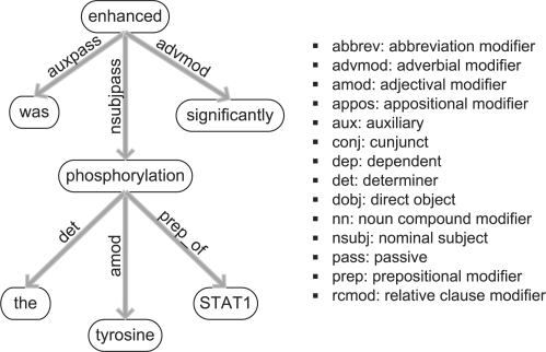
To enable in-depth analysis of grammatical structures using dependency parsing, we have included the Stanford parser (de Marneffe et al., 2006) in our framework. The dependency graph of a sentence contains the informative words of the sentence as nodes, while the edges express grammatical relations between those words. Dependency parsing is widely used for extracting relations from text, as it provides a compact and informative representation of the sentence structure. An exemplary dependency graph is depicted in Figure 2.

Fig. 2.

Dependency graph for the sentence ‘The tyrosine phosphorylation of STAT1 was enhanced significantly.’ Words of the sentence form the nodes of the graph, while edges denote their syntactic dependencies. The most frequently occurring dependency abbreviations are listed on the right.

2.3 Instance creation

Candidate events are formed by combining a trigger with GGPs co-occurring in the same sentence. These trigger words are selected from a dictionary created from training data. To compose such a dictionary, we calculate the importance of an event trigger t_i for a particular event type T: Imp(t^T_i) = f(t^T_i)/∑_p=0ⁿf(t^T_p), where f(t^T_i) is the frequency of the event trigger t_i of event type T in a training corpus, divided by the total number n of all event triggers of that type T in the training corpus (i = 0,…, n). Subsequently, we apply a cut-off value of 0.005, keeping only those triggers that are sufficiently informative.

2.4 Feature generation

For each candidate event in the training data, the feature generation module extracts various patterns, including bag-of-word (BOW) features, trigrams, vertex walks and information about the event trigger. These patterns are subsequently used as matching criteria when building the feature vectors for the test set.

As the various feature types and their relative importance for classification are the main topic of this article, we present a short overview in this section, while referring to Van Landeghem et al. (2010) for details.

2.4.1 Trigram features

Trigrams are formed by combining three consecutive words in the subsentence delimited by the trigger and GGP offsets in the text. They capture common phrases, e.g. ‘high levels of’. GGP names are blinded in the text, meaning that the GGP name is substituted by the string ‘protx’, e.g. ‘transcription of protx’.

2.4.2 Trigger features

1. The specific event trigger is highly relevant to the classifier, thus its lexical tokens are added as features (e.g. ‘degradation’).

2. The part-of-speech tags of the trigger words are also included as syntactic features (e.g. ‘noun’).

2.4.3 Vertex walks

To incorporate information derived from dependency parsing, we analyze the smallest subgraph including all relevant nodes for the trigger and the GGP names. For each edge in this subgraph, we create a pattern using the information from the nodes in combination with the specific dependency relation.

1. For the lexical variant, blinding is applied to trigger words and GGP names, resulting in highly general patterns such as ‘trigger preposition-of protx’.

2. The syntactic counter-part uses the part-of-speech tags of the words on the nodes, e.g. ‘noun preposition-of noun’.

2.4.4 BOW features

BOW features incorporate all words occurring as nodes on the dependency subgraph. They include highly informative words such as ‘heterodimers’.

A final post-processing step in the feature generation module applies stemming to all lexical patterns, using the Porter stemming algorithm (Porter, 1980). This algorithm maps words to their stem by applying a suffix-striping algorithm (e.g. ‘homodimer’ is the stem of ‘homodimerization’). On top of blinding certain words (e.g. protein names), stemming further generalizes the feature patterns. Generalization is crucial for a text mining framework, as it enables extraction and prediction of events concerning previously unpublished genes.

Table 1 presents an overview of the datasets. The number of instances ranges from 264 to 6895, while the dimensionality of the feature sets lies between 1826 and 29 941 features, correlating strongly with the number of instances. Finally, class balance varies from only 7% positives to 51% positives.

Table 1.

Dimensionality of the various datasets

Dataset	Total number	Percentage	Size of
	of instances	of positives (%)	feature set
Catabolism	264	39	1826
Phosphorylation	318	51	2121
Binary binding	2332	8	10 958
Unary binding	3612	14	20 058
Localization	3791	39	18 537
Expression	6347	25	28 384
Transcription	6895	7	29 941

Binding events are covered by two distinct data sets, involving either one (‘unary’) or two (‘binary’) distinct GGPs.

2.5 Feature selection

To perform FS we used the recently introduced concept of ensemble FS (Saeys et al., 2008) for which implementations are available in Java-ML (Abeel et al., 2009). Ensemble FS builds on the idea of ensemble classification by using multiple weak feature selectors to build a single robust one. These weak feature selectors are created by bootstrapping the training data and then building an SVM. The weights of the support vectors determine the rank of the features, and individual rankings are aggregated in a consensus ranking using linear aggregation (Abeel et al., 2010). Bootstrapping is done as sampling with replacement to obtain a bootstrap of the same size as the training set. Training sets for the individual runs are created by sampling without replacing 90% of the entire training set.

Stability of feature rankings is measured using the consistency index as defined by Kuncheva (2007):

where f_i and f_j are the top features of ensemble ranking i and j, s = |f_i| = |f_j| denotes the signature size, r = |f_i ∩ f_j| equals the number of common elements in both signatures and N represents the original number of features. A higher Kuncheva index indicates a larger number of commonly selected features in both signatures.

The signature size can either be expressed as the total number of retained features, or as the percentage of the feature space that is retained after FS. For knowledge discovery, we typically want the signature size to be small enough to analyze manually. For classification, however, classification performance and feature reduction have to be optimized jointly.

2.6 Classification and evaluation

Our datasets consist of thousands of instances and thousands of features (Table 1). On top of these high-dimensional properties, there is a class imbalance of up to 93% negatives. To classify this data, we used the SVM implementation from LibSVM (Chang and Lin, 2001) as provided in WEKA (Hall et al., 2009). A radial basis function is selected as kernel for this binary classifier and parameter tuning is implemented with a 5-fold cross-validation loop on the training data (Van Landeghem et al., 2010).

The final predictions are evaluated by the golden standard evaluation script provided by the BioNLP'09 ST organizers, which provides precision, recall and F-measure for each event type individually, while also calculating global performance over all event types together.

3 RESULTS

This section presents the main results of our study. First, we discuss the results for FS stability (Section 3.1) and describe the classification results of the enhanced framework (Section 3.2). Further, Section 3.3 discusses the relative importance of the various feature types and finally, Section 3.4 offers many in-depth analyses of the discriminative power of individual features.

3.1 Stable FS

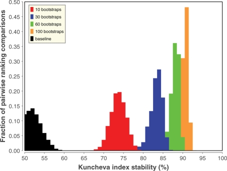
Figure 3 plots the distribution of the FS stability in function of the number of bootstraps used for the consensus ranking. From this figure, it is clear that using more bootstraps to create the consensus ranking has a beneficial effect on the stability of the selected features. Even though there are still small gains, the stability improvements seem to saturate at about 60 bootstraps.

Fig. 3.

FS stability improvements by using more bootstraps for the unary binding event. Distributions are plotted for 10, 30, 60 and 100 bootstraps and the baseline FS when retaining 25% of the features. The stability is measured with the Kuncheva index between all pairwise combinations of consensus rankings. Similar graphs are obtained for the other six datasets.

While the figure is generated from the dataset on unary binding, similar graphs are obtained for the other six datasets (data not shown). The increase in stability from baseline to a 100 bootstrap consensus ranking is between 20% (on the transcription set) and 43% (on the protein catabolism set). More stable FS means less variation of the selected features, which has two main benefits. First of all, stable FS identifies more meaningful features and allows the construction of better performing classifiers (Section 3.2). Furthermore, it enhances the interpretability of the selected features (Sections 3.3 and 3.4).

3.2 Enhanced accuracy and reduced dimensionality of event classification

When irrelevant features can be eliminated from the dataset, an SVM should have an easier task distinguishing true predictions from false ones, resulting not only in faster classifiers but also in enhanced performance. To test this hypothesis, we evaluated the performance of the classifier when using only a small fraction of the original feature space. We compare these results with the global baseline performance of our system (65.02% F-score). This baseline is a strong performing classifier to compare against, as it is produced by the system ranking third out of 24 participants in this subchallenge of the BioNLP'09 Shared Task (Kim et al., 2009).

Table 2 presents the classification results when incorporating FS. Evaluation is performed on 100 distinct FS runs, and the table reports on minimum, maximum and average performance across these runs. The calculated average values clearly show that FS improves the classification performance: the combined model consistently outperforms the baseline performance at signature sizes of ≥20%. Further experiments indicated that performance peaks around 25% of the feature space with minimal variance between the folds (data not shown). Performance starts dropping below baseline with a signature size of about 10%.

Table 2.

Classification performance for all 100 FS runs, showing minimum, maximum and average performance for global event extraction

Signature	Minimum	Maximum	Average
size (%)	F-measure (%)	F-measure (%)	F-measure (%)
75	64.85	65.33	65.26
50	65.60	66.43	65.88
30	64.94	66.60	65.86
25	65.51	66.82	66.14
20	65.08	66.56	65.85
10	61.75	64.90	63.59

The initial baseline without FS is 65.02 F-score.

These results prove that our FS algorithm successfully discards irrelevant features, producing a dimensionality reduction of 75% and average classification improvement of 1.12% F-score. As this result validates the output of the FS algorithm, it also creates the opportunity to analyze the top-ranked features in more detail. By analyzing which features are highly important to the SVM, we will be able to gain some insight into this ‘black box’ algorithm. This is not only beneficial for the end-user, providing clues why events are predicted, but will also be applicable for enhancing the implementation of ML frameworks for event extraction. Both applications are discussed in the next two sections.

3.3 Relative importance of feature types

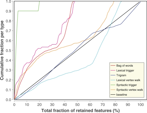
Section 2.4 discussed the various classes of feature types used in our framework. To assess the relative importance of each type, we have analyzed the consensus ranking produced by aggregating the results of the 100 FS runs. Figure 4 details the results for the dataset on unary binding. Highly similar graphs were obtained for the other datasets and overall conclusions follow the same trend.

Fig. 4.

FS order for the dataset on unary binding. The x-axis shows the total fraction of selected features in the feature set, while the y-axis displays the fraction of features of one specific feature type. The black line indicates a random FS baseline method.

Figure 4 depicts the relative rate at which each of the feature types is being selected at each step of the FS algorithm. This analysis shows that the features expressing syntactic information about the trigger words (Section 2.4.2.2) are overrepresented in the top-ranked features, i.e. they are being selected first. About 90% of all syntactic triggers are present in the top 5% of the consensus ranking and all of them are present within the top 20% features.

At <50% of the total feature space, all lexical information about triggers (Section 2.4.2.1) as well as all BOW features (Section 2.4.4) are also selected. Consequently, these feature types appear to be highly relevant and include practically no irrelevant features.

Vertex walks express grammatical relations between the words of the dependency graphs. The features of the syntactic variant (Section 2.4.3.2) are highly overrepresented in the top 20% of the ranking, but their relative increase diminishes afterwards. The lexical counterpart (Section 2.4.3.1) appears to be much less informative in general.

Finally, trigrams (Section 2.4.1) resemble the baseline in the top 70% of the features, and form the entire last 20% of the ranking. Obviously, the feature generation method produces many irrelevant trigrams. We have analyzed these bottom-ranked trigrams and found that many originated from three subsequent words spanning multiple phrases, such as ‘subunits and the’. Here, the conjunctive ‘and’ links two distinct noun phrases, and it could thus be more beneficial to extract trigrams only from within the same noun or verb phrase (e.g. ‘interacts directly with’).

3.4 Individually discriminating features

To gain even deeper insight into the most discriminating features, we have analyzed the feature ranking for each distinct event type across all 100 folds. For each ranking, the top 100 features were taken into account. Even though this top 100 is generally too small to capture the complexity of event extraction in a classification setting, analysis of the most frequently occurring features in the top 100 provides strong clues of the most discriminating features and allows us to learn interesting aspects of the feature generation process.

Each individual feature appearing at least once in the top 100 is assigned a score, by counting the number of times it occurs in a top 100 and assigning higher weights to higher ranked features. Subsequently, we have generated tag clouds of these features, scaling their font size according to their weight, and applying a color-coding scheme that shows whether the feature mainly occurs in negative samples (bright red), in positive samples (blue) or equally in both (purple). To correct for the large class imbalance present in most datasets, we have normalized the actual rate with the expected rate in each dataset, by taking into account the specific class distribution.

In this section, we will discuss some of the most interesting tag clouds in detail. The chosen tag clouds represent various event types as well as various feature types, and the words appearing in them are transformed to their stemmed and lowercase variants.

Figure 5 shows the most informative trigger words for the Localization dataset, identifying crucial words such as ‘local(ization)’ and ‘secret(ion)’ as highly relevant trigger words for this dataset. However, at the same time we notice that ‘express’ and ‘presenc/t’ also rank high, but indicate negative events. Consequently, these trigger words should probably have been eliminated from the dictionaries in the first place. Indeed, the formula for Imp(t^T_i) does not take into account the balance between positive and negative examples for a certain trigger (Section 2.3). It would thus be beneficial to incorporate this information into the formula, eliminating negative candidate events even before classification, while at the same time reducing the dimensionality of the datasets. However, this is a complex problem as the frequency of trigger words is likely to be different in the training and testing data.

Fig. 5.

The most discriminative lexical triggers for localization events.

There is another lesson to be learned from Figure 5: two stemmed words ‘presenc’ and ‘present’ are treated as distinct triggers, even though they refer to a similar concept. This finding indicates an important shortcoming of stemming, which applies simple suffix-striping rules but does not map similar concepts to the same word. However, lemmatization could solve this problem and provide even better generalization of the feature vectors.

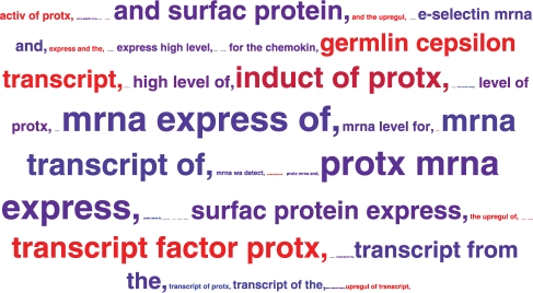
As a next example, Figure 6 presents the most informative trigrams for the transcription dataset. The pattern ‘transcript factor protx’ strongly hints toward a negative example, as it indicates that the text defines the protein as a particular transcription factor rather than actually discussing transcription of that protein.

Fig. 6.

The most discriminative trigrams for transcription events.

In contrast, the framework has found several interesting positive patterns involving mRNA expression. ‘mRNA’ is also selected as the most informative BOW feature for transcription (data not shown). This clearly shows that our framework is capable of deducing relevant biological knowledge from the training data, without having to turn to external databases or expert knowledge. This characteristic is very valuable, as an ideal text mining framework does not rely on any external information, but can instead process information not yet indexed in external databases.

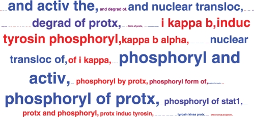
The tag cloud for trigrams in the phosphorylation dataset shows similar examples involving ‘i kappa b alpha’ (Fig. 7), while immediately indicating a limitation of the feature representation: patterns of more than three words cannot be efficiently captured. While the various parts are present (‘i kappa b’ and ‘kappa b alpha’), it could be valuable to create additional features considering N-grams with N > 3 in a new version of the text mining algorithm.

Fig. 7.

The most discriminative trigrams for phosphorylation events.

An additional problem is caused by the heterogeneity of word usage by various authors, an intrinsic property of natural language. Indeed, in some of the text, ‘i kappa b alpha’ is referred to as ‘iKappaBAlpha’, ‘IkappaB-alpha’ or ‘I kappa B-alpha’. Our current feature vectors are incapable of linking these terms to the same concept. Again, a lemmatization or dictionary look-up approach could prove to be of value in these cases.

Further analyzing other lexical patterns of the Phosphorylation trigrams, we find the pattern ‘phosphoryl of protx’ to indicate a strong positive, while ‘phosphoryl by protx’ leads to negative events. While this seems counter-intuitive at first sight, it can be explained by taking the definition of the Phosphorylation event into account: the argument of the event should always be the protein that is phosphorylated. In terms of the BioNLP'09 Shared Task data, the pattern ‘phosphoryl by protx’ would lead to a regulation event in which a protein regulates phosphorylation of yet another protein. Even though these regulation events are out-of-scope for the current study, we conclude that the classifier correctly labels them as negatives in the Phosphorylation dataset.

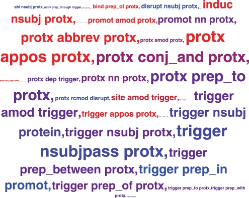
Finally, interesting linguistic patterns can be found when analyzing the tag cloud of lexical vertex walks in the dataset on binary binding (Fig. 8). When a direct link exists between the two proteins involved, this strongly points to a negative example (e.g. ‘protx conj_and protx’ or ‘protx abbrev protx’). On the other hand, the nature of the link between a trigger and a protein is highly informative (e.g. ‘trigger prep_between protx’ or ‘protx nsubj protx’). We note that most of the highly ranked vertex walks involve nodes that have been blinded, confirming the usefulness of the blinding step to improve generalization (Section 2.4).

Fig. 8.

The most discriminative lexical vertex walks for (binary) binding events.

4 DISCUSSION AND CONCLUSION

This article presents the first extensive study on FS applied to event extraction from biomedical texts. Thorough analyses have shown that our FS method based on SVMs correctly models feature interdependencies and is thus well suited to tackle text mining challenges. We have shown that our FS approach can eliminate up to 90% of all features before it drops below the baseline without FS. Classification improves most when eliminating 75% of all features, considerably reducing dimensionality of the datasets. This peak is not at the same cutoff for all datasets and future work could explore how this signature size can be optimized for each individual event type.

While FS stability is a valuable asset of an analysis as it improves the analytical power of experts, it is crucial to optimize it in conjunction with classification performance. It is trivial to create a perfectly stable feature selector by always taking the first x features, but such a feature selector would never offer new insights. However, we have shown that our ensemble FS approach not only provides more robust feature selectors, but also improves classification performance and provides insight into the predictions of the black box model of ML methods.

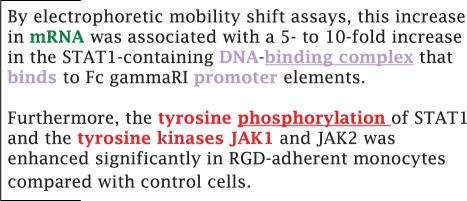
Analysis of the top selected features has shown various interesting characteristics, both in terms of biology and from a linguistic point of view. Some of these insights are illustrated in Figure 9, which depicts a text sample highlighting top-ranked features. These lexical constructs provide interesting clues about predicted events and help the reader to better understand the nature of the predictions made by the SVM classifier.

Fig. 9.

Text example from PMID:9278334. Three distinct event types are discussed: transcription (green, previous sentence), binding (purple, first sentence) and phosphorylation (red, second sentence). The relevant trigger words are ‘binding complex’ and ‘phosphorylation’ (underlined). Relevant BOW features include ‘mRNA’, ‘DNA’, ‘binds’, ‘promoter’ and ‘tyrosine’. Finally, there is a match with the trigram ‘tyrosin kinas protx’. All highlighted words help the reader find relevant clues for each event type.

Furthermore, the feature analysis has given us an in-depth understanding of the feature generation algorithms and ideas on how to improve on these. Our analyses have shown a number of interesting shortcomings in current feature generation algorithms. As an example, improvements to the trigger detection algorithm would allow us to reduce the number of candidate events as these sentences will no longer be considered to be putative candidate events and the classification model can focus in truly distinguishing between candidates. However, due to the complex nature of the event extraction task and varying properties between training and test set, improving trigger dictionaries is far from trivial.

Another shortcoming that should be addressed is the use of stemming. Clearly ‘present’ and ‘presenc’ both represent the same concept, but they occur as separate features when using stemming, which—though widely used—essentially just removes suffixes. Lemmatization would provide a viable alternative, further reducing the sparseness of the feature vectors and creating more general feature patterns. Unfortunately, lemmatization requires a lot more work up-front as it needs a complete vocabulary and morphological analysis to correctly lemmatize words.

An additional improvement for the lexical features could be the inclusion of N-grams for N > 3. Trigrams are unable to capture word groups longer than three words, while the feature clouds indicate that such features could be relevant for classification. It would additionally make sense for all N-grams to only include patterns extracted from within a single phrase. We regard the numerous opportunities for improvement discussed in this article as interesting future work.

To conclude, we would like to reiterate that stable FS enables an in-depth analysis of discriminative features and provides insight in the different steps of biomedical text mining. Furthermore, our FS algorithms allow us to build more cost-efficient classifiers which outperform baseline classifiers while only using a fraction of the features. Finally, stable feature selectors can guide the user of prediction software through the results of automatic discovery by highlighting discriminative features used during classification.

Funding: Research Foundation Flanders (FWO) (to S.V.L. and Y.S.); IWT-Vlaanderen (to T.A.).

Conflict of Interest: none declared.

REFERENCES

- Abeel T, et al. Java-ML: a machine learning library. J. Mach. Learn. Res. 2009;10:931–934. [Google Scholar]
- Abeel T, et al. Robust biomarker identification for cancer diagnosis with ensemble feature selection methods. Bioinformatics. 2010;26:392–398. doi: 10.1093/bioinformatics/btp630. [DOI] [PubMed] [Google Scholar]
- Airola A, et al. All-paths graph kernel for protein-protein interaction extraction with evaluation of cross-corpus learning. BMC Bioinformatics. 2008;9(Suppl. 11):S2. doi: 10.1186/1471-2105-9-S11-S2. [DOI] [PMC free article] [PubMed] [Google Scholar]
- Chang C-C, Lin C-J. LIBSVM: a library for support vector machines. 2001 Available at http://www.csie.ntu.edu.tw/∼cjlin/libsvm (last accessed date July 20, 2010) [Google Scholar]
- Cohen KB, et al. BioNLP '09: Proceedings of the Workshop on BioNLP. Morristown, NJ, USA: Association for Computational Linguistics; 2009. High-precision biological event extraction with a concept recognizer; pp. 50–58. [Google Scholar]
- de Marneffe M, et al. Proceedings of LREC-06. Genoa, Italy: 2006. Generating typed dependency parses from phrase structure parses; pp. 449–454. [Google Scholar]
- Hall M, et al. The weka data mining software: an update. SIGKDD Explorations. 2009;11:10–18. [Google Scholar]
- Kim J-D, et al. Proceedings of the BioNLP 2009 Workshop Companion Volume for Shared Task. Boulder, Colorado: Association for Computational Linguistics; 2009. Overview of bionlp'09 shared task on event extraction; pp. 1–9. [Google Scholar]
- Krallinger M, et al. Evaluation of text mining systems for biology: overview of the second biocreative community challenge. Genome Biol. 2008;9(Suppl. 2):S1. doi: 10.1186/gb-2008-9-s2-s1. [DOI] [PMC free article] [PubMed] [Google Scholar]
- Krallinger M, et al. Analysis of biological processes and diseases using text mining approaches. Methods Mol. Biol. 2009;593:341–382. doi: 10.1007/978-1-60327-194-3_16. [DOI] [PubMed] [Google Scholar]
- Kuncheva L. Proceedings of the 25th International Multi-Conference on Artificial Intelligence and Applications. Anaheim, CA, USA: ACTA Press; 2007. A stability index for feature selection; pp. 390–395. [Google Scholar]
- Porter MF. An algorithm for suffix stripping. Program. 1980;14:130–137. [Google Scholar]
- Reverter A, et al. Mining tissue specificity, gene connectivity and disease association to reveal a set of genes that modify the action of disease causing genes. BioData Min. 2008;1:8. doi: 10.1186/1756-0381-1-8. [DOI] [PMC free article] [PubMed] [Google Scholar]
- Saetre R, et al. Proceedings of the 2nd International Symposium on Languages in Biology and Medicine (LBM) Singapore: 2008. Syntactic features for protein-protein interaction extraction. [Google Scholar]
- Saeys Y, et al. Machine Learning and Knowledge Discovry in Databases. Berlin/Heidelberg: Springer; 2008. Robust feature selection using ensemble feature selection techniques; pp. 313–325. Vol. 5212 of Lecture Notes in Computer Science. [Google Scholar]
- Van Landeghem S, et al. Proceedings of the Third International Symposium on Semantic Mining in Biomedicine (SMBM) Turku, Finland: Turku Centre for Computer Sciences (TUCS); 2008. Extracting protein-protein interactions from text using rich feature vectors and feature selection; pp. 77–84. [Google Scholar]
- Van Landeghem S, et al. High-precision bio-molecular event extraction from text using parallel binary classifiers. Computational Intelligence. 2010 (in press) [Google Scholar]