A varying threshold method for ChIP peak-calling using multiple sources of information

Abstract

Motivation: Gene regulation commonly involves interaction among DNA, proteins and biochemical conditions. Using chromatin immunoprecipitation (ChIP) technologies, protein–DNA interactions are routinely detected in the genome scale. Computational methods that detect weak protein-binding signals and simultaneously maintain a high specificity yet remain to be challenging. An attractive approach is to incorporate biologically relevant data, such as protein co-occupancy, to improve the power of protein-binding detection. We call the additional data related with the target protein binding as supporting tracks.

Results: We propose a novel but rigorous statistical method to identify protein occupancy in ChIP data using multiple supporting tracks (PASS2). We demonstrate that utilizing biologically related information can significantly increase the discovery of true protein-binding sites, while still maintaining a desired level of false positive calls. Applying the method to GATA1 restoration in mouse erythroid cell line, we detected many new GATA1-binding sites using GATA1 co-occupancy data.

Availability: http://stat.psu.edu/∼yuzhang/pass2.tar

Contact: yuzhang@stat.psu.edu

1 INTRODUCTION

Understanding the association between protein occupancy and the target gene expression is essential to study the mechanism of gene regulation. The first step is to identify the protein-binding sites in the genome. Current chromatin immunoprecipitation (ChIP) technologies coupled with microarray hybridization (ChIP-chip) or parallel DNA sequencing (ChIP-seq) enable the identification of transcription factor-binding sites in vivo in the genome-wide scale. Many computational methods have been developed to detect transcription factor occupancy from ChIP-chip and ChIP-seq data, which we refer to as peak calling. Making choices of program parameters and choosing significance thresholds to accurately control genome-wide false positives (FPs), however, is often difficult. We have previously developed a statistical method (Zhang, 2008) that can precisely control the expected number of genome-wide FP peak calls in the context of correlated multiple comparisons. With FPs controlled, it is further desired to improve the peak calling methods to reduce false negative instances.

Gene regulation is a complex process that usually involves the cooperation of multiple transcription factors, which may interact to form a regulatory module that binds to a DNA segment to regulate their target gene's expression. Certain histone modifications may also play crucial roles in regulatory mechanisms (Heintzman et al., 2007; Muller et al., 2002). The binding potential of a target transcription factor, therefore, can be partially learned from the co-binding proteins and features that jointly participate in a regulatory module within the cell. As the prevalent ChIP technologies increase the need for analyzing ChIP-chip and ChIP-seq data, several studies have made efforts to utilize multiple biological features into ChIP data analysis. For example, methods have been developed for segmenting the genomic regions into active intervals of interest (Day et al., 2007; Du et al., 2006). Few methods for peak calling, however, have incorporated the joint effects of related biological features while detecting binding sites for a target protein. Datta and Zhao (2008) have proposed a method that uses a log-linear model to infer co-binding associations between two or more transcription factors. Their method is a post-processing algorithm that takes the P-values from existing peak calling algorithms as input, but cannot incorporate general types of data.

In this article, we propose a novel yet rigorous method that accounts for the co-binding information and relevant biological features to detect DNA occupancy of a target protein from ChIP data. Without assuming distributions of the related biological features, which we call supporting tracks, we first use a logistic regression model to describe the correlation between the binding of the target protein and the supporting tracks. The output is the probability of each position being potentially occupied by the target protein, predicted by the supporting tracks. We then introduce a varying threshold method to call significant peaks from the ChIP data of interest, where the threshold for each probe is adjusted by its predicted probability of protein binding. Our approach is similar to that of a Bayesian method that incorporates prior knowledge of protein binding into the analysis. Different from Bayesian methods, we still control the family wise FP rate, or false discovery rate (FDR) (Benjamini and Hochberg, 1995), at a user-specified level. Our varying threshold method, called PASS2, is a generalization from the PASS algorithm (Zhang, 2008), and is related with conditional test in statistics (Cox and Hinkley, 1979).

Using simulation studies and real datasets of GATA1 binding in a mouse erythroid regulation study (Cheng et al., 2009), we show that the proposed method can identify many more GATA1-binding sites than using the target ChIP data alone, when the FDR is controlled at a common level. Our study shows that the proposed framework is robust with respect to irrelevant supporting data added to the model. The additional binding sites detected by incorporating the related biological features are potentially real GATA1-binding sites, many of which are either experimentally verified or enriched near RefSeq Genes (Pruitt et al., 2007). To our best knowledge, the proposed method is the only algorithm that incorporates multiple sources of information in peak calling to improve the power of detecting weak protein-binding signals, and simultaneously, our method controls a user-specified FP level adjusting for millions of correlated comparisons.

2 METHODS

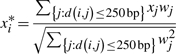
We assume the ChIP data of interest and the supporting tracks are generated by independent experiments. We first map all tracks of data onto a common coordinate represented by tiling probes. Here, we use the term ‘probe’ to represent a short genomic interval (≤100 bp) that corresponds to the probes used in ChIP-chip experiments. A probe for ChIP-seq experiments and for other types of data can be arbitrarily defined. To convert each track of data into probe statistics, we calculate a standardized value (t_i) at each probe i by taking the average value of the original data (x_j) within the probe interval, and dividing the average value by its SD. The SD is calculated as the SD (σ) of all data in the track divided by the square root of the number of data points (w) within the probe interval:

(1)

For computational efficiency and model robustness, we further apply discretization methods to convert the continuous values of supporting tracks into ordinal bins. We then apply a logistic regression model to compute the binding probability of each probe being occupied by the target protein, using the binned supporting data as predictors and a list of known or highly probable binary binding sites of the protein as the response. We use permutation to evaluate the relevance of supporting tracks, and we discard insignificant tracks. We finally calculate a probe-specific threshold for each probe according to the calculated binding probabilities. We use the probe-specific thresholds to call significant peaks from the ChIP data of interest. A flow chart of our method is shown in Figure 1.

Fig. 1.

Flow chart of the proposed method.

2.1 Discretization methods

To efficiently represent a large number of unique values generated by the genome-wide arrays, we categorized continuous values of supporting tracks into bins to reduce the size of data matrix. Binning data also improves the robustness of binding site prediction by reducing the effects of extreme values in the supporting data. We applied different discretization techniques and compared their effects on the performance of peak calling. Unsupervised discretization methods such as equal-width or equal-frequency methods, and clustering algorithms, require a specified number of bins for discretization. We evaluated the performance of unsupervised methods using different number of bins. We also applied an entropy-based discretization method that utilizes the known binding sites in a supervised manner to determine an optimal number of bins and assignment of bins based on information content maximization (Fayyad and Irani, 1993).

2.1.1 Equal-width and equal-freq method

let k denote the number of bins, the ‘Equal-Width’ method partitions the range of continuous values into k intervals of equal width. The ‘Equal-Freq’ method, on the other hand, assigns an approximately equal number of continuous values in each bin.

2.1.2 Clustering method

a k-means clustering algorithm is used to assign all continuous values into k bins. For k = 2, the minimum and the maximum values in a supporting track are used as the cluster centroids. For k > 2, the initial k cluster centroids are the values, including the minimum and maximum values that partition the data into (k − 1) bins of equal width.

2.1.3 Entropy method

given a sorted array of continuous values S and a corresponding array of binding status of the target protein, the method finds a best cut point T that partitions the range of S into two non-overlapping intervals. A cut point T is the midpoint between two contiguous data points in the sorted array. For each candidate cut point T, the data are divided into two subsets on each side of T. The class entropy of a subset S_j, where ‘class’ refers to the binding status, is defined as

(2)

here, c denotes the number of classes (c = 2), and p_i denotes the proportion of data points in S_j that belong to class i. The entropy of a bi-partition of S at cut point T is then defined as the weighted average of the class entropies of subset S₁ and S₂:

(3)

where |S| denotes the size of array S. The partition that minimizes Ent(S, T) over all cut points T is selected as the best partition.

Define the information gain of a partition at cut point T as

(4)

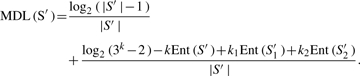
Our goal is to find a best split of data that maximizes the information gain. The algorithm is applied recursively within each partitioned interval to find sub-partitions, until some stopping criteria are satisfied. The algorithm uses the minimum description length (MDL) as a criterion for accepting or rejecting a given partition. The partition by a cut point T is accepted if and only if Gain(S′, T) > MDL(S′), where MDL(S′) is calculated as

(5)

here, S₁′ and S₂′ denote a best bipartition of S′, and k, k₁, k₂ (= 1 or 2) denote the number of distinct classes in S′, S₁ and S₂, respectively. The algorithm stops when no more partitions satisfying the MDL constraints can be found.

The supporting tracks were binned individually while running the above four discretization methods. To use the entropy-based discretization, each track of data was sorted, and a list of known or predicted binding sites was mapped to the probe coordinate and used as the class label c of each data point. We only evaluated the cut points at the boundary between two classes (boundary of binding sites), because the cut point T that minimizes the average class entropy Ent(S, T) is always a value between two data points of different classes in a sorted array (Fayyad and Irani, 1993).

2.2 Prediction of potential binding

To combine information from the supporting tracks and predict the binding locations of a target protein, we fit a logistic regression model between a vector of binary indicators Y = (Y₁, Y₂,…, Y_n) denoting the known binding status of the target protein at n probes, and a data matrix X of m supporting tracks. Each column of X, denoted by X_i = (X_i1, X_i2,…, X_in)', contains the converted bin values of the i-th supporting track at n probes, for I = 1,…, m. The vector Y can be constructed from experimentally verified binding events, previous studies of the target protein occupancy or computationally detected sites from the current ChIP data at a stringent threshold. When computationally detecting binding sites as the responses in training data, a stringent FDR should be controlled so that the fitted regression model will not be strongly biased towards FPs. We suggest using a FDR no larger than the FDR allowed at the end of peak-calling. For example, if 10% FDR is allowed at final peak calling, then the initial peak-calling for training should be controlled at 10% FDR. The rationale is that, even if training peaks are FPs, they are still allowed at final peak calling.

We model the binding events Y of the target protein at n probes as independent Bernoulli random events with parameter π, where π denotes an n-dim vector of binding probabilities. We model π as a function of supporting tracks X via a logistic link function as

(6)

and hence

(7)

where β₀ denotes the baseline binding coefficient and β_i denotes the additional effect of binding contributed by the supporting data X_i.

The parameters β = (β₀,…, β_m) were estimated by maximum likelihood estimation. Since the data points are generally correlated, we used permutation test to evaluate the empirical significance of the effect of each supporting track X_i, and we removed insignificant tracks from the model at 0.01 significance level.

2.3 Varying thresholds for peak calling

Given the effects β of supporting tracks, we can calculate a vector π of binding probabilities of the target protein at all probes in the ChIP data. We use the same notation π to denote the binding probability of probes in the ChIP data, for which significant peaks are to be called, where the π used in the previous section corresponds to the training probes that are used to fit the logistic regression model.

We generalized the original PASS algorithm (Zhang, 2008) to utilize the binding information predicted by the supporting tracks. By default, we assume that the probe values in the ChIP data have been standardized to follow a normal distribution at unbound regions. A probe (or a window of probes) is called statistically significant if its statistic (or the average statistic of a window) is above a threshold. Intuitively, if a probe has a higher probability to be occupied, we may reduce its peak-calling threshold so that the probe is easier to be called and hence reduce the chance of false negatives. The key is to choose the probe-specific thresholds according to the predicted binding probabilities of probes, and at the same time control the overall number of FPs at a user-specified level.

The difficulty of controlling the overall FP rate in peak calling arises from the fact that the probe values are locally strongly correlated. The original PASS algorithm (Zhang, 2008) uses a de-clumping method to compensate the positive correlations among probes, such that the total number of FPs after de-clumping can be simply computed as a summation of the FP rate of individual probes. We slightly modified the de-clumping method as follows: we now call a probe significant if and only if its statistic is above a threshold and is the maximum among probes within its neighborhood. As a result, for all probes within any local interval, at most one probe can be called significant (assuming no ties) under this rule, and hence the positive correlation among probes is compensated. All theoretical treatments stated in the original PASS paper (Zhang, 2008) still hold true under this new de-clumping scheme. Ignoring local interference of negative correlations created by de-clumping, and based on the fact that a probe being significant by chance is rare, we can approximate the expected total number of FPs in the entire ChIP data by summing over the FP rate of individual probes. It further holds true that the family wise FP rate of peak calling, with or without de-clumping, remain unchanged (Zhang, 2008), and hence our method can control both family wise FP rate and FDR.

To utilize the predicted binding probabilities, and to control the overall number of FPs at a desired level λ, we choose probe-specific thresholds as follows. For each probe i, we calculate a threshold t_i such that probe i has probability α_i = min(1, λπ_i/|π|) to be a FP by chance after de-clumping, where |π| denotes to the summation of elements in π. This can be done by calculating the significance of a range of thresholds at probe i, using the importance-sampling algorithm proposed in PASS (Zhang, 2008). We then use interpolation to compute t_i that yields α_i.

To use the varying thresholds t_i in peak calling, we call a probe significant (occupied by the protein) if its test statistics is greater than or equal to t_i and is the maximum within its neighborhood (500 bp by default). The expected total number of FPs of all probes can therefore be approximated as

(8)

As a result, we can control the overall number of FP calls at a user-defined level λ. At the same time, we gain a substantial amount of power in detecting genuine protein-binding sites by using a liberal threshold at probes that are likely to be occupied, as suggested by the supporting data. To control family wise FP rate at level α _FWER, we let λ = −log(1 − α_FWER) and calculate varying thresholds with respect to λ at individual probes. To control FDR at α level, we use a step-down approach as follows: (i) start at λ = α, we calculate the varying thresholds and report all peaks passing the thresholds; (ii) we increase λ to λ = kα, where k denotes the total number of peaks detected in previous iterations, and we recalculate the varying thresholds and call more peaks; and (iii) we repeat step 2 until no more peaks can be found.

2.4 ChIP data and supporting data

The target ChIP data and the supporting data are generated from the same mouse erythroid cell line with restoration of GATA1 function (G1E-ER4). We applied our method to two real studies, one ChIP-chip data and one ChIP-seq data, to detect GATA1 occupancy in the mouse genome. GATA1 is a transcription factor that regulates erythroid genes. The ChIP-chip data was obtained from a hybridized GATA1 ChIP sample to the NimbleGen HD2 tiling array for the mouse genome (mm8 assembly). The ChIP-seq data was obtained from a different GATA1 biological sample sequenced by Illumina GAII technology, with 23 million 36 bp reads uniquely mapped to the mouse genome (mm8 assembly) (Cheng et al., 2009).

We further obtained four additional datasets that are related with GATA1 binding and are used as supporting tracks: (i) DNase-seq open chromatin data from F-Seq (Boyle et al., 2008a, b); (ii) ChIP-seq data of TAL1 (also known as SCL) that often co-binds with GATA1, LDB1 and LMO2 to form a multi-protein complex (Wadman et al., 1997); (iii) ChIP-seq data of trimethylation of lysine 4 of histone H3 (H3K4me3) associated with active promoters (Heintzman et al., 2007); and (iv) ChIP-seq data of trimethylation of histone H3K27 (H3k27me3) associated with down-regulation (Muller et al., 2002). The data tracks used in this study contained 883 758 probes in a previously reported 66 Mb region on mouse chromosome 7. This region contains a large number of experimentally verified GATA1-binding sites (Cheng et al., 2008), and hence servers as a good example to demonstrate our method.

The ChIP-seq data contained discrete counts of short reads mapped to consecutive positions in the genome. To apply our method, we converted the GATA1 ChIP-seq read counts to probe statistics as follows: (i) calculate the sum of read counts according to a defined probe coordinate; (ii) with top 1% probes of large read counts removed, model the background distribution of read counts by a negative binomial distribution, NB(r, p), and estimate the two parameters p and r by maximum likelihood estimation; (iii) compute the P-value of each probe from the assumed background distribution and converted the P-values to Z-scores. Our method allows the user to specify the probe size and ‘tiling’ resolution. In general, larger distance between probes (e.g. 100 bp) may lose ChIP-seq signals and therefore reduce the power of peak detection. Conversely, smaller distance between probes (e.g. 1 bp) will not compromise mapping resolution, but could be computationally intensive. Probe size should not be too small so that it contains enough tag counts. By default, we use a probe size of 30 bp tiled at every 10 bp distance for ChIP-seq data, and we recommend using a window of 2–5 probes to call peaks. Users can change these values in our program.

3 RESULTS

3.1 Simulation study

We first performed simulation study to evaluate the power and the robustness of our method. We generated random ChIP-chip data containing 883 758 probes, among which 300 randomly selected probes corresponded to protein-binding sites. For probes at the binding and non-binding sites, we simulated the probe intensities from a normal distribution with mean 8 and 0, respectively, and variance 1. To further introduce correlation among probes, each probe value was replaced by a weighted average within its 500 bp window, calculated as

(9)

where w = 1 when i = j, w = 0.8 when d(i, j) ≤ 125 bp and w = 0.4 when d(i, j) > 125 bp.

The signals in the simulated data ranged from −5.28 to 8.13 with mean 0.0046 and variance 1.02. This is comparable with the ChIP-chip HD2 data (ranged from −11.77 to 8.29 after normalization). Since the simulated binding sites were randomly placed, they were independent with the four supporting tracks. We therefore can evaluate the impact of using irrelevant supporting tracks in peak calling. In particular, we did not remove the unrelated supporting tracks when calculating the binding probabilities, and we checked whether using the irrelevant information can increase the number of FPs by our method. We used the ‘Equal-Freq’ method to discretize each supporting data into k = 7 bins, and we called significant peaks at 10% FDR level. We further compared our method with an existing method, MPeak (Zheng et al., 2007, trimming P-value set at 1e-05) on the same datasets.

As shown in Figure 2, the estimated FDR (number of FPs/number of detected peaks) level of our method was accurately controlled at the specified 10% level, and the FDR level remained invariant before and after incorporating irrelevant supporting information. In each simulated dataset, our method detected an average of 240 (out of 300) true peaks. As we expected, the number of peaks detected before and after using irrelevant data remained almost unchanged (first column in Fig. 3). This result indicates that our method can accurately control FPs with and without using additional information, and the method is robust to irrelevant data added to the model. In comparison, MPeak reported an average of 210 peaks per dataset, among which only 135 were true peaks, pertaining to ∼36% FPs.

Fig. 2.

Comparison of FDRs in 10 simulated datasets. Our method with and without using supporting tracks (prior) is controlled at 10% FDR level. We cannot specify FDR level for MPeak.

Fig. 3.

(A) FDR and (B) detection power comparison of our method before (black) and after (colored) using supporting tracks at different levels of concordance. Box-plot of 10 datasets at each concordance level is shown.

We next evaluated the power of our method by introducing correlation between the binding sites and the supporting data. Out of 300 binding sites in each simulation study, x% binding sites were randomly placed at locations of previously identified GATA1-binding sites from real GATA1 ChIP-chip HD2 data (Cheng et al., 2009). The remaining (100 − x)% binding sites were placed at random locations. We varied x from 0% to 100% with a 20% increment. For each x value, we generated 10 ChIP-chip datasets using the method described above. Since the four supporting tracks were significantly correlated with GATA1 binding, they were correlated with the simulated binding sites at varying levels.

We applied our method to each simulated dataset, with insignificant supporting features removed by permutations, except for x = 0%, and we called significant peaks at 10% FDR level. As shown in Figure 3A, we observed that the actual FDR level for each simulated datasets remained around 10% or less at varying concordance levels. As shown in Figure 3B, after incorporating supporting features in peak calling, our method detected many more (up to an additional 20%) true peaks that were missed by conventional methods. The gain of power is an increasing function with respect to the absolute correlation between the protein-binding data and the supporting data.

3.2 Performance of discretization methods

To evaluate the peaks detected by our method in real data analysis, we constructed a positive set of 99 true GATA1 occupied segments validated by qPCR in G1E-ER4 cells in a previous study (Zhang et al., 2009). The ChIP data used to identify those 99 validated peaks (VPs) was different from the ChIP-chip HD2 data analyzed in this article, and hence the VPs do not necessarily show strong signals in our HD2 data. In fact, we observed that the ChIP-chip HD2 intensity of the 99 VPs ranged from 0.32 to 4.07, where the entire ChIP-chip HD2 signals ranged from −5.76 to 4.07. The wide range of signals observed from the VPs provides us a good reference set to evaluate our method. We further partitioned the VPs into three groups: (i) high VPs: 53 true sites with probe intensities >2 in ChIP-chip HD2 data; (ii) medium VPs: 24 true sites with probe intensities between 1.5 and 2; and (iii) low VPs: 22 true sites with probe intensities <1.5. We also constructed a negative set of 83 FPs-binding sites that failed the previous validation of qPCR (Cheng et al., 2008; Zhang et al., 2009). Some of these 83 FPs, however, showed large signals in our ChIP-chip HD2 data and hence may be weak GATA1-binding sites. In addition to those positive and negative validation peaks, we also compared our results with results obtained using existing methods on the same ChIP-chip and ChIP-seq data (Cheng et al., 2009).

We first evaluated the impacts of discretization methods on peak calling. We conducted independent peak-calling experiments on the ChIP-chip HD2 data using various discretization methods on the four supporting tracks. We first ran the PASS program (Zhang, 2008) to detect peaks at 10% FDR level. We then fit the output to a logistic regression model with the four supporting tracks as covariates. The following methods were used to discretize the supporting data: (i) round each probe value to the nearest integer (‘Round’); (ii) calculate the average value (t_i) of a 1000 bp window of each probe and round the value to integer (‘SmoothRound’); (iii) use the four methods (‘Equal-Width’, ‘Equal-Freq’, ‘Clustering’ and ‘Entropy’) described in Section 2.

As shown in Figure 4, when evaluated at the same FDR level, ‘Entropy’ and ‘Equal-Freq’ outperformed other methods in terms of the number of detected peaks, medium VPs and peaks overlapping with previously identified ChIP-seq peaks (Cheng et al., 2009). ‘Equal-Width’ performed the worst, but still slightly outperformed the conventional method. The results of Round, SmoothRound and Clustering were better than the conventional method, but worse than Entropy and Equal-Freq methods. Our results indicated that a proper choice of discretization method is important, as it have significant impacts on peak-calling results.

Fig. 4.

Comparison of peak-calling performance using six different discretization methods on supporting tracks: Equal-Width, Equal-Freq, Clustering (k = 2 ∼ 8), Entropy, Round and SmoothRound. The traditional peak-calling method without using supporting tracks (no prior) is shown as a comparison. (A) The total number of detected peaks. (B) The total number of detected true peaks with medium intensity (1.5–2.0). (C) The total number of detected peaks overlapping with previously identified ChIP-seq peaks.

3.3 Novel peaks detected by supporting tracks

By incorporating the 4 GATA1-related supporting tracks, we identified a total of 125 novel GATA1-binding sites, of which 66 sites were identified from the ChIP-chip data and 63 sites were identified from the ChIP-seq data (Table 1). Before using supporting tracks, 14 out of 24 VPs with medium intensity were detected by the original PASS program at 10% FDR level. Two additional VPs with medium intensity lied within 400 bp of the PASS detected peaks. After using supporting data, our method captured four (out of the remaining eight) more VPs with medium intensity. The other four missing VPs were hard to detect from the ChIP-chip HD2 data and were also missed by the previous ChIP-chip analysis (Cheng et al., 2009). They were only detected from the ChIP-seq data (Cheng et al., 2009).

Table 1.

Predicted GATA1-binding sites enrichment in true binding regions, RefSeq Gene and predicted peaks by Cheng et al. (2009)

Dataset	Number of peaks	Number of high VPs	Number of medium VPs	Number of low VPs	Total VPs	Number of FP	ChIP-chip peaks	ChIP-Seq peaks	Union of peaks	RefSeq genes
		53	24	22	99	83	311a	780a	890a	1176
ChIP-chip peaks
PASS—no prior	317	51	14	0	65	4	251	221	292	198/149
PASS2—additional	66	0	4	0	4	1	19	33	44	43/38
MPeaks	147	45	8	0	53	2	142	112	145	91/74
TMAL (L1)	139	40	9	1	50	1	134	97	137	84/41
ChIP-seq peaks
PASS—no prior	554	45	16	13	74	4	177	463	467	325/186
PASS2—additional	63	0	0	0	0	0	5	35	35	36/33

^aComputationally identified peaks by Cheng et al. (2009).

VPs, validated peaks by q-PCR (Cheng et al., 2008; Zhang et al., 2009); RefSeq Genes, RefSeq genes from the UCSC browser in the 66 Mb region on chromosome 7 in the mouse genome (mm8). Overlapping entries are merged. The overlapping intervals between RefSeq genes and the detected peaks have P-value < 0.05 from 100 permutations.

For VPs of high intensity in the ChIP-chip data, our method with and without using supporting tracks performed equally—51 out of 53 VPs overlapped with our detected peaks. For VPs of weak intensity, none were detected by our method with or without using supporting tracks. From the ChIP-seq data, however, we detected 13 VPs (60%) of low intensity. Although we found more GATA1-binding sites from the ChIP-seq data than from the ChIP-chip data, it is worthy of noting that the true peaks found in ChIP-chip data were not completely captured by the ChIP-seq data, and vice versa.

To further evaluate the novel peaks found by the supporting tracks, we compared our results with peaks found in a previous study (Cheng et al., 2009). Of the 66 additional ChIP-chip peaks, 50% (33/66) overlapped with the previously identified ChIP-seq peaks, 65% (43/66) overlapped with 38 RefSeq Genes. Similar results were observed in the 63 additional ChIP-seq peaks. We also compared our results with MPeak and TAMALPAIS (Bieda et al. 2006). The two programs, however, do not directly provide FDR control. For MPeak, we used its P-value in the output to compute FDR assuming independence between tests. At 10% FDR threshold, MPeak detected 147 peaks when their P-value cutoff is around 1.6e-05. For TAMALPAIS, we used the most stringent threshold (L1) and detected 139 peaks. Compared to PASS2, MPeak and TAMALPAIS (L1) were both conservative.

For the effects of the four supporting tracks, as shown in Table 2, the open chromatin, H3k4me3 and TAL1 all had positive effects on GATA1 binding, where H3K27me3 as a repressor had negative effect on GATA1 binding. We observed that the effect of the open chromatin data and the GATA1-binding status in the ChIP-chip was different from that in the ChIP-seq data. The inconsistency may be attributable to the difference in noise levels and the bias in ChIP-chip and ChIP-seq experiments.

Table 2.

Estimated effects and P-values of the supporting tracks

	ChIP-chip		ChIP-seq
	β	P-value	β	P-value
Intercept	−1.25e+01	0	−1.14e+01	0
Open chromatin	2.42e−02	6.73e−01	6.70e−01	5.26e−48
H3K27me3	−2.63e−01	9.78e−06	−1.51e+00	1.25e−12
H3K4me3	1.79e+00	1.36e−106	1.18e+00	9.45e−34
TAL1	7.99e−01	2.46e−67	1.51e+00	3.26e−246

β is the regression coefficient in the logistic regression model.

Among the 554 ChIP-seq peaks that were originally detected by PASS, three peaks were redefined by our method at shifted nearby locations (Fig. 5A). The raw ChIP-seq data around the three sites showed double-peak distributions. As suggested by the supporting data, the new binding sites defined by PASS2 were more likely to be occupied by GATA1.We show in Figure 5B one example of the novel peaks found by our method. The GATA1 occupied segment in this region was validated by qPCR and had a max ChIP-chip intensity of 1.77. The region, however, was missed by a previous study using both ChIP-chip HD2 data and ChIP-seq data (Cheng et al., 2009). The original PASS program also missed this region. This GATA1 occupied segment is located within gene ‘Tjp1’, which is depleted of H3K27me3 but enriched with open chromatin and H3K4me3 signals. After incorporating the related feature tracks, we recovered this true GATA1-binding site using the proposed method.

Fig. 5.

(A) Venn diagram of the ChIP-chip and ChIP-seq peaks identified with and without the supporting tracks. (B) An example of a novel GATA1-occupied segment within Tjp1 identified by our method. It was missed by previous HD2 ChIP-chip and ChIP-seq analysis (Cheng et al., 2009). This region also shows depleted H3K27me3 and enriched H3K4me3 signals. Horizontal black lines indicate signal means.

4 DISCUSSION

We introduced a new statistical method to improve the power of detecting protein binding in ChIP data by combining additional biological features. The proposed method not only improves the sensitivity of peak calling than traditional methods, but also precisely controls a user-specified level of FP rate or FDR. The additional sites detected by our method are those regions with medium- or low-binding signals, which cannot pass the genome-wide statistical significance control. After taking into account of the correlation between the binding sites and biologically related supporting features, regions coincide with strong supporting signals will become detectable by our method.

Using both simulation and real data analysis, we observed that our method can effectively detect 20% more true binding sites than traditional peak-calling methods. Under all scenarios we tested, our method also precisely controlled the proportion of FP calls at 10% FDR level. We further observed that the proposed method is robust to irrelevant data tracks added to the model.

Our method does neither assume any distributions on the supporting data nor it attempts to estimate data distributions empirically. Such assumptions and estimation procedures may introduce unwanted bias and uncertainty in peak calling. Our method is flexible to incorporate any types of biological information that overlap with the ChIP regions. By converting continuous data into bins, the binding probabilities computed from our logistic regression model will be robust to outliers and extreme values. Our analysis showed that a proper discretization method applied to supporting tracks can also have significant impact on peak calling results. Instead of applying discretization to individual supporting tracks (univariate discretization), multi-variate discretization methods that take into account of the interaction among features could be used to capture the missing patterns from univariate approaches (Bay, 2001).

The real data analysis we performed in this study was based on ChIP-chip data and a ChIP-seq data in 66 Mb region on the mouse chromosome 7. This region contained a substantial amount of GATA1- and TAL1-binding sites compared to other regions (Cheng et al., 2008). This is a focal region for investigating the interaction between proteins and is a best region to test our method. We used GATA1 peaks detected at a stringent threshold to train the model parameters to avoid using many FPs in fitting the logistic regression model. It is possible that the fitted regression model may be biased towards strong binding sites. The underlying assumption of our method, therefore, is that the fitted model from strong peaks will have predictive power to weak binding sites. The worst scenario will occur when weak binding sites have completely opposite supporting data distribution compared to that of strong binding sites, in which case the fitted regression model will predict against the weak binding sites. This is a common issue that will occur to all methods that rely on training data, if the training data and the testing data are heterogeneous. In our method, we attempted to alleviate this problem by repeating the process of peak-calling, fitting regression and peak-calling again, iteratively, such that if weak binding sites are detected at some iteration, their information will be included in the training of regression model, and a new iteration of peak-calling will be applied. The novel peaks found by our method was a set of candidate peaks of weaker binding events. It is still unclear whether the binding strength of a transcription factor can affect gene regulation. The weak peaks detected by our method therefore provide a source of information for investigating this association. The logistical regression model we fitted in this region can be further applied to predict genome-wide GATA1 occupancy.

There are currently a large number of computational methods developed for detecting protein–DNA interactions in ChIP experiments. Most methods did not provide a rigorous means to control FP detections. The PASS algorithm (Zhang, 2008) solved this problem in the context of correlated multiple comparisons. The detected statistically significant binding intervals, however, may not correspond well to the real biological binding sites. The method proposed in this study attempts to improve both sensitivity and specificity of peak calling by incorporating biologically related information. The proposed framework is flexible in terms of accommodating various types of data as supporting tracks, and is also flexible in terms of the methods used at each step of the algorithm. Instead of using a logistic regression model to predict binding of the target protein, statistical or machine-learning classifiers can be used to measure the potential of protein binding at each probe from the supporting data. We then fit the predicted binding potentials into the varying threshold framework to determine probe-specific thresholds.

With the advancement of next-generation sequencing technologies, researchers are now able to generate a huge amount of data of various biological features of interest, including ChIP data for multiple transcription factors, histone modifications, nucleosome positioning and RNA-seq. These feature tracks are usually highly correlated and jointly provide valuable information for answering some of the fundamental questions in gene regulation. The proposed method is an example of integrating such information to increase the power and specificity in peak detection.

Funding: National Human Genome Research Institute (grants R01 DK065806 to Y.Z. and HG002238 to K.C., in part).

Conflict of Interest: none declared.

REFERENCES

- Bay SD. Multivariate discretization for set mining. Knowl. Inf. Syst. 2001;3:491–512. [Google Scholar]
- Benjamini Y, Hochberg Y. Controlling the false discovery rate: a practical and powerful approach to multiple testing. J. Roy. Stat. Soc. Ser. B. 1995;57:289–300. [Google Scholar]
- Bieda M, et al. Unbiased locationanalysis of E2F1-binding sites suggests a widespread role for E2F1 in the human genome. Genome Res. 2006;16:595–605. doi: 10.1101/gr.4887606. [DOI] [PMC free article] [PubMed] [Google Scholar]
- Boyle AP, et al. High-resolution mapping and characterization of open chromatin across the genome. Cell. 2008a;132:311–322. doi: 10.1016/j.cell.2007.12.014. [DOI] [PMC free article] [PubMed] [Google Scholar]
- Boyle AP, et al. F-Seq: a feature density estimator for high-throughput sequence tags. Bioinformatics. 2008b;24:2537–2538. doi: 10.1093/bioinformatics/btn480. [DOI] [PMC free article] [PubMed] [Google Scholar]
- Cheng Y, et al. Transcriptional enhancement by GATA1-occupied DNA segments is strongly associated with evolutionary constraint on the binding site motif. Genome Res. 2008;18:1896–1905. doi: 10.1101/gr.083089.108. [DOI] [PMC free article] [PubMed] [Google Scholar]
- Cheng Y, et al. Erythroid GATA1 function revealed by genome-wide analysis of transcription factor occupancy, histone modifications, and mRNA expression. Genome Res. 2009;19:2172–2184. doi: 10.1101/gr.098921.109. [DOI] [PMC free article] [PubMed] [Google Scholar]
- Cox D, Hinkley D. Theoretical Statistics. London: Chapman and Hall; 1979. [Google Scholar]
- Datta D, Zhao H. Statistical methods to infer cooperative binding among transcription factors in Saccharomyces cerevisiae. Bioinformatics. 2008;24:545–552. doi: 10.1093/bioinformatics/btm523. [DOI] [PubMed] [Google Scholar]
- Day N, et al. Unsupervised segmentation of continuous genomic data. Bioinformatics. 2007;23:1424–1426. doi: 10.1093/bioinformatics/btm096. [DOI] [PubMed] [Google Scholar]
- Du J, et al. A supervised hidden markov model framework for efficiently segmenting tiling array data in transcriptional and chIP-chip experiments: systematically incorporating validated biological knowledge. Bioinformatics. 2006;22:3016–3024. doi: 10.1093/bioinformatics/btl515. [DOI] [PubMed] [Google Scholar]
- Fayyad UM, Irani KB. Proceedings of the 13th International Conference on Artificial Intelligence. France: Chambéry; 1993. Multi-Interval discretization of continuous-valued attributes for classification learning; pp. 1022–1027. [Google Scholar]
- Heintzman ND, et al. Distinct and predictive chromatin signatures of transcriptional promoters and enhancers in the human genome. Nat. Genet. 2007;39:311–318. doi: 10.1038/ng1966. [DOI] [PubMed] [Google Scholar]
- Muller J, et al. Histone methyltransferase activity of a Drosophila Polycomb group repressor complex. Cell. 2002;111:197–208. doi: 10.1016/s0092-8674(02)00976-5. [DOI] [PubMed] [Google Scholar]
- Pruitt KD, et al. NCBI reference sequences (RefSeq): a curated non-redundant sequence database of genomes, transcripts and proteins. Nucleic Acids Res. 2007;35:61–65. doi: 10.1093/nar/gkl842. [DOI] [PMC free article] [PubMed] [Google Scholar]
- Wadman IA, et al. The LIM-only protein Lmo2 is a bridging molecule assembling an erythroid, DNA-binding complex which includes the TAL1, E47, GATA-1 and Ldb1/NLI proteins. EMBO J. 1997;16:3145–3157. doi: 10.1093/emboj/16.11.3145. [DOI] [PMC free article] [PubMed] [Google Scholar]
- Zhang Y. Poisson approximation for significance in genome-wide ChIP-chip tiling arrays. Bioinformatics. 2008;24:2825–2831. doi: 10.1093/bioinformatics/btn549. [DOI] [PubMed] [Google Scholar]
- Zhang Y, et al. Primary sequence and epigenetic determinants of in vivo occupancy of genomic DNA by GATA1. Nucleic Acids Res. 2009;37:7024–7038. doi: 10.1093/nar/gkp747. [DOI] [PMC free article] [PubMed] [Google Scholar]
- Zheng M, et al. ChIP-chip: data, model, and analysis. Biometrics. 2007;63:787–796. doi: 10.1111/j.1541-0420.2007.00768.x. [DOI] [PubMed] [Google Scholar]