Discriminatory power of RNA family models

Abstract

Motivation: RNA family models group nucleotide sequences that share a common biological function. These models can be used to find new sequences belonging to the same family. To succeed in this task, a model needs to exhibit high sensitivity as well as high specificity. As model construction is guided by a manual process, a number of problems can occur, such as the introduction of more than one model for the same family or poorly constructed models. We explore the Rfam database to discover such problems.

Results: Our main contribution is in the definition of the discriminatory power of RNA family models, together with a first algorithm for its computation. In addition, we present calculations across the whole Rfam database that show several families lacking high specificity when compared to other families. We give a list of these clusters of families and provide a tentative explanation. Our program can be used to: (i) make sure that new models are not equivalent to any model already present in the database; and (ii) new models are not simply submodels of existing families.

Availability: www.tbi.univie.ac.at/software/cmcompare/. The code is licensed under the GPLv3. Results for the whole Rfam database and supporting scripts are available together with the software.

Contact: choener@tbi.univie.ac.at

1 INTRODUCTION

Structured non-coding RNAs are nucleotide sequences that are not translated into protein but have, in the folded state, their own specific functions (Mattick and Makunin, 2006). This function is very much dependent on the secondary and tertiary structure (the folded state), while on the other hand, the primary structure or sequence sees more change (Mattick and Makunin, 2006) in the form of mutation.

One can define relationships between non-coding RNAs in different species. A set of related sequences is called an RNA family. Each set is defined by its members performing the same function in different species. When genomes are sequenced, one is interested in finding members of known families in the new data, as well as finding new families if previously unknown non-coding RNAs are discovered.

The problem—finding homologues—exists for proteins, too. Software to perform the same kind of searches exists in the form of HMMer (Eddy, 1998) and the Pfam (Bateman et al., 2002) database. Using profile hidden Markov models (profile HMMs), a mathematically convenient solution was found, around which the algorithms could be built. Unfortunately, the same solution proved inadequate (Durbin et al., 1998, Chapter 10.3) for non-coding RNAs.

The task of building a model that describes a new family is still a mostly manual process. Finding new members of existing families, on the other hand, can be performed using software. The problem we are discussing in this article applies equally well to other algorithms to search for homologue sequences, but as our algorithm is specific toward an existing software package, namely Infernal (Nawrocki et al., 2009a), we will perform our analysis with respect to this software and the corresponding Rfam (Griffiths-Jones et al., 2003) database.

In order to model families of non-coding RNAs in a way that provides both sensitivity and specificity, the consensus secondary structure of the set of sequences has to be included in the mathematical model from which the algorithm is created. Stochastic context-free grammars provide access to such models, just as stochastic regular grammars (in the form of profile HMMs) can be used to model protein families.

We begin with a succinct introduction to the process of first designing an Infernal RNA family model and then searching for new family members. Building on those algorithms, we can define the specificity of a given model compared to other known models in a natural way using the already established Infernal language of bit scores.

1.1 Infernal model design

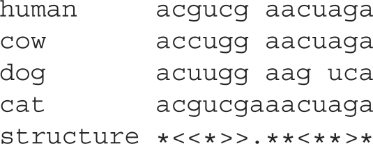
Infernal is based on covariance models (Eddy and Durbin, 1994). We assume that a structure-annotated multiple alignment of the family sequences like the one in Figure 1 is at hand. Intuitively, new family members should (i) align well and (ii) show the same secondary structure. The more a sequence deviates from these two requirements the worse it should score.

Fig. 1.

Multiple alignment of sequences from several species and the consensus structure. Brackets denote nucleotide pairings, a star denotes a consensus unpaired nucleotide and a dot a nucleotide not in the consensus.

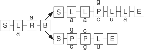
During the covariance model construction process, a so-called guide tree is derived from the structure annotation. The nodes of the tree fall into six classes: (1) a pair-matching (P) node for a base pair; (2–3) two kinds of single nucleotide nodes, one left- (L) and one right-matching (R); (4) a bifurcation (B) node to allow for multiple external and internal loops; and two house-keeping nodes: (5) a start-node (S) and (6) an end-node (E). Whenever possible, left-matching nodes are used, e.g. in hairpin loops, delegating right-matching nodes to be used only where necessary, such as the right side of the last external loop. This removes ambiguity from the construction process. The alignment from Figure 1 leads to the model depicted in Figure 2.

Fig. 2.

A covariance model, displaying the six types of nodes needed for construction. The nucleotide annotation follows the human sequence of the multiple alignment of Figure 1.

Mutations in base pairs or single conserved nucleotides are handled in the conventional stochastic RNA modeling approach by keeping emission probabilities (or log-odd scores) for each possible base or pair for the emitting nodes (P, L, R).

The way Infernal works, insertion of additional nucleotides or deletion of parts of the consensus sequence cannot be handled by the matching nodes alone. For the final model, each node is replaced by a number of states. One state acts as the main state, that is, for example, each pair (P) node has a pair state matching both a left and a right nucleotide. The deletion of one of the two nucleotides is handled by adding two states, one only left- (L), one only right-matching (R). A fourth state (D) handles the deletion of both nucleotides while two inserting states (IL, IR) are used for insertions relative to the consensus. Transitions from one state to the next happen with some probability which is close to 1.0 for the consensus state and far less likely for the other possible states. The exact numbers are calculated by fitting probability distributions using the multiple alignment data.

Nodes matching only a single nucleotide are extended with a deletion state and either a left- or a right-inserting state, depending on the main state. A bifurcation (B) leads directly to two new start (S) nodes, effectively to two complete submodels. By arbitrary selection, the right start node is extended with a left-inserting state to allow for insertions between a bifurcation.

Mostly, however, it is enough to keep the picture of the model (Fig. 2), using only matching nodes, in mind.

With the additional states the model is completed. The fitting of the probability distributions given the nucleotide consensus data is outside of the scope of this text and we refer the reader to the book on the subject matter by Durbin et al. (1998).

1.2 Searching with covariance models

The complete model is a graphical representation of the stochastic context-free grammar that does the real work. A pair state (P), for example leads to a total of 16 productions of the form P_k → aQb, where P_k is the k'th node to be processed, Q abstracts over the possible targets states, which depend on the node k + 1 and (a, b) are the 16 possible nucleotide pairs. The whole process leads to CFGs with a huge number of productions (in the order of the number of nodes times a small constant), especially when compared with single RNA folding grammars (Dowell and Eddy, 2004), that have in the order of 10–100 productions.

The actual search process uses the CYK algorithm (newer versions of Infernal use the Inside algorithm to calculate the final score) to find the best parse of an input string given the model. Input strings are all substrings of a genome up to a given length. Using dynamic programming, this approach is fast enough that whole genomes can be processed in a matter of hours or days.

Our interest in this article is not the search process of Infernal, but how a parse is scored and the best alignment of string against model is selected.

Notation. —

Given an alphabet 𝒜, 𝒜^* denotes the set of all strings over 𝒜. Let s ∈ 𝒜^* be a, possibly empty, input string.

Notation. —

Let m, m₁, m₂ be covariance models in the form of stochastic context-free grammars conforming to the Infernal definition.

Given a model m and an input string s, the CYK score can be calculated over all parses ¶ of the string s by the model m:

(1)

A successful parse is a parse that consumes the complete input s and finishes in terminal end states. During such a parse a score is built up from the transition and emission scores that were calculated for each model during its construction.

Several methods exist to perform the calculations. Arguably, closer to Equation (1) is the use of tree grammars and algebras in Giegerich and Höner zu Siederdissen (2010), but Infernal uses traditional dynamic programming to implement the CYK algorithm. Whichever method is used, they are more efficient than the enumeration of all possible parses. Finally, the alignment of the input against the model can be retrieved using backtracking or other methods.

2 METHOD

A covariance model with high specificity assigns low bit scores to all sequences that do not belong to the model family. Finding sequences that lead to false positives, that is having a high score while not belonging to the family, is a problem. We take a view that does not look at a single model, but rather at two models at the same time. Then, we can say that:

A covariance model has low specificity with respect to another model if there exists a sequence s ∈ 𝒜^* that achieves a high CYK score in both models.

We acknowledge that ‘high score’ is not well-defined, but consider what constitutes a high score in Infernal. Hits in Infernal come as a tuple, the score itself and an e-value. One is typically interested in scores of 20 bit or higher and e-values of 1.0 or less, depending on the model. The e-value is dependent on the genome size, but given such guidelines one finds good candidates. In light of this, the meaning of ‘high score’ becomes more clear. As we use the same measure as Infernal, a string that achieves, say, 40 bit in two different models points to low specificity, as the string would be considered a good hit when searching for new family members with both models separately.

Using the previous definition, we find an analog to Equation (1) to calculate (i) the highest score achievable by (ii) a single input string:

(2)

Here, m₁ and m₂ are two different covariance models. MaxiMin returns the highest scoring string. The highest score is defined as the minimum of the two CYK scores. This guarantees that both models score high. Variants of the algorithm are possible, for example MaxPlus which sums both scores before maximizing. However, MaxiMin provides better results in case one of the two models contains many more nodes than the other. More importantly, it provides a score which would actually be achieved during a search using one of the two models, while the other would score even higher. As the sequence s ‘links’ both models via their discriminative power, we shall use the term Link from now on.

The trivial implementation suggested by Equation (2) is not well-suited for implementation as it requires exponential runtime due to the enumeration of all possible strings in 𝒜^*.

In order to find the highest scoring string, we perform a kind of tree alignment with additional sequence information. The tree alignment part optimizes the structure of each model, while sequence alignment is performed for nucleotide emitting states as well. Both alignments are tightly coupled as is the case for covariance models themselves. A pair state (P), for example, leads to another structure than a left-emitting (L) state. This also explains why we have to deal with a small restriction in our algorithm. The tree alignment requires us to align each state with at most one other state, but not two or more. After an explanation of the implementation, we discuss this further.

Implementation:

We present a simplified version of our recursive algorithm in Table 1. To set the field, we need two additional functions. Equation (3) defines the minimum of a pair of values in a natural way. The function maxmin [Equation (4)] is a small helper function selecting the maximal pair, where the maximum of two pairs is defined by the maximum of individual minima, hence the name max-min.

Table 1.

Recursive calculation of the maximal score achieved by an input string common to both model m₁ and m₂

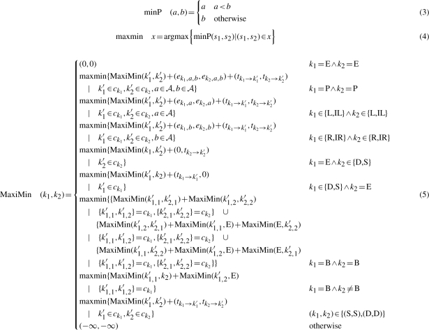We abuse notation quite a bit to reduce notational clutter. The state type of model 1 at index k would be but we write k₁ = E to determine if the state is an end state. Additional data structures are simplified as well. The states into which a transition is possible (the children of state k) are written c_k1 instead of c¹_k1. Emission scores for each model are in the matrix e which is indexed by the state k and the nucleotide(s) of the emitting state. Transition scores for transition from state k to k′ are found in the matrix t. The case where k₁ = E ∧ k₂ = E terminates the recursion, as each correctly built covariance model terminates (each submodel) with an end-state (E) (cf. Fig. 2). Addition of pairs happens element-wise: (a, b) + (c, d) = (a+b, c+d).

The recursion has to be performed simultaneously over both models. For model m₁ we have index k₁ and for model m₂, k₂ will be used. Note though, that by following just one of the elements of the tuples, the CYK algorithm can be recovered. We are, in essence, performing two coupled CYK calculations at the same time.

Internally, all states are kept in an array. The first index is guaranteed to be a start state (S) and the last index to be an end state (E). The first state is the root state of the whole model, too. Three additional arrays are required.

The states that can be reached from a state are stored in an array named c for children. Because indices from one model are never used in the other model, we can always write c_k1 instead of c_k1¹.

We use the same simplification for emission scores. The array e holds such scores. It is indexed with the nucleotides that are to be emitted. This is to be written as e_k1,a,b for pairs and either a or b are missing for single nucleotide emitting states.

The third required array, t, stores transition scores. Whenever the recursion descends from a state k₁ into a possible child state k₁′, a lookup t_k1→k1′ is performed. Not all transitions incur a cost. A branch into the two child states always happens with probability 1.0.

We have abused notation to simplify the recursion a bit. The determination of the type of the current state requires an additional data structure to perform the lookup for the indices k. Instead of writing X_k1, where X is such a data structure, we just write k₁ = E to assess if state k₁ happens to be an end (E) state.

Some of the cases found in the source code have been removed for clarity. Most cases deal with symmetric states. The last state to visit is, for example (E, E). This initializes the CYK score to (0.0, 0.0). The case (MP, MP) handles the emission of a pair of nucleotides. There are some cases like (S, x), where x is any state except (S), that require special handling. These special cases ((E, D) and (E, S) are given as an example) do not contribute any information on how one goes about calculating the common score, but simply make a large recursion more unwieldy.

The algorithm is asymptotically fast. Given the number of states n₁ and n₂ of the two models, each pair of states will be visited once at most. In addition, the number of children c_k1 and c_k2 per state is fixed by a constant. If h denotes the maximal number of children per state, the total runtime is bounded by O(n₁n₂h²).

A restriction in the implementation:

Consider the structure annotation of two different covariance models: ma: < < > > and mb: * < > *. Model m_a has two nodes P₁^a – P₂^a and model m_b three nodes: L₁^b – R₂^b – P₃^b. An input string like ccgg is likely to result in a good score for both models, especially if we assume that the family sequences are similar to ccgg. Equation (2) would return that result after some time. For a fast implementation, those two models are rather inconvenient as P₂^a has to be matched against both L₁^b and R₂^b at the same time. By allowing to match only one state against one other state, our algorithm produces suboptimal scores in such cases. Fortunately, this is a minor problem for real models. This can be explained by the relative scarcity of such cases and the regularity of the covariance model building process. If left-matching and right-matching nodes could be used at will, e.g. in hairpin loops, our simplification would have more than minor consequences.

Local and global scoring:

Infernal does not require that a sequence matches the whole model. Instead, a local search is performed. Each string is aligned against the part of the model where it scores best. Should this require the deletion of parts of the model, this does not invoke many delete (D) states. One can simply do a transition into a local start or end state. These transitions are possible only with small probability (typically around 0.05 divided by the number of nodes in the model) but this still gives higher scores than potentially having to descend into dozens of delete states.

Since Infernal scores locally with respect to the model, we do the same by default. Details of the implementation are omitted. Using the –global switch, this behaviour can be changed. In that case, both models have to be aligned and the resulting string will be optimal with respect to the whole model, not just some submodel. Several other switches known from Infernal are available, too.

Just one string?:

Of course if only a single string has a good score in both models, the problem would be moot as the probability to encounter that exact string is close to zero. But consider that from the pairwise score and the corresponding string, suboptimal strings can be generated easily. Given the length k of the string s, then k points for substitutions give 3k strings that score almost as high. A further strings score less, and so forth with 3 and more substitutions. Furthermore, insertions and deletions are possible.

This means that whenever there is one high-scoring string, there will be many more, we just present the worst case.

3 RESULTS

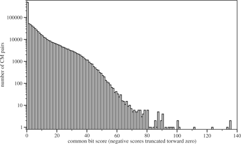
The Rfam 9.1 database contains 1372 different models. All pairwise calculations lead to a total of 940 506 results. The time to calculate the score and string for each pair is typically less than one second, but of course depending on the size of the models in question. Of all pairs, about 70 000 are noteworthy with scores of 20 bit or more. Figure 3 shows the distribution of scores among all pairs of family models. Negative scores have been truncated towards zero as any score lower than this certainly means that the two models in question are separated very well.

Fig. 3.

Distribution of bit scores for all 940 506 pairs of covariance models. About 70 000 pairs have scores of 20 bit or more, pointing towards weak separation between the two models.

Among the high-scoring pairs are several interesting examples, some of which we will take a closer look at. Similar results for other models can be extracted from the data available for download. It is possible to generate, among others, model-centric views that show the high-scoring neighborhood of a particular model and global views that show high-scoring pairs. As Figure 4 aptly demonstrates, clusters of families form early (in this case, only the 20 highest scoring edges are drawn).

Fig. 4.

The 20 highest scoring edges between RNA families. Each edge represents a string that, between the connected nodes, results in a bit score at least as high as the given value. The two connected family models have low discrimination in such a case. For each family model the Rfam index and name are shown.

In Table 2, we have gathered some results. The 70 000 pair scores over 20 bit have been split according to the abstract shape of the secondary structures of the hit. A shape (Reeder and Giegerich, 2005) is a representation of the secondary structure that abstracts over stem and interior loop sizes. In this case, each pair of brackets defines one stem. Intervening unpaired nucleotides do not lead to the creation of a new stem. Hits such as _/_ are unstructured, but similar, sequences. The shape []/[] is just one hairpin, while the two shapes [[][]]/[[][]] on the same string point to an interesting pair score as the string apparently folds into complex high-scoring structures that align well, too.

Table 2.

Occurrence of shapes in results with at least 20 bit each

m1	_	[]	[][]	[][][]	[[][]]	Complex
m2	_	[]	[][]	[][][]	[[][]]	Complex
Found	19 644	49 289	1576	40	12	28

Unstructured regions (dashes) and hairpins (square brackets) as the common region occur most often. The other shapes show that complex substructures can form. The high number of lone hairpin structures is a direct consequence of the huge meta-family of snoRNAs which have a simple secondary structure. Under ‘complex’, all structures that did not fit into the given shapes were collected.

In principle, it is possible that the common sequence folds into two different secondary structures. At abstract shape level 5 (the most abstract) this did not happen for the current Rfam database. Our algorithm, however, is capable to deal with such cases.

Let us now take a closer look at two examples that are particularly interesting. The first was selected because RNaseP is a ubiquitous endoribonuclease and the second to highlight how problematic models can be discovered.

1 st example:

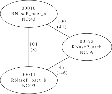
The RNaseP families for bacteria (type a and b) and archaea show weak separation as can be seen in Figure 5. The three involved models (Rfam id 10, 11 and 373) have different noise cutoff scores. The noise cutoff is the highest score for a false hit in the Rfam NR database, scores above this threshold are likely homologues (cf. Nawrocki et al., 2009b).For the three different RNaseP families, these scores are 43, 93 and 59 bit, respectively. A look at Figure 5 shows, that no random sequence could score high in both model 373 and 11, one can, at most, find a hit that is remote at best. The picture is entirely different for the high-scoring sequence between RNaseP, type a and RNaseP in archaea. Here, we find a sequence that is at least 41 bit higher than the noise cutoff. A similar picture presents itself for the sequence found for the two bacterial RNaseP models, though the score difference between the noise cutoff and the highest score is only 8 bit.

Fig. 5.

Link scores for different RNaseP models (with noise cutoff (NC)) with weak separation. Values in brackets are the difference to the noise cutoff thresholds. The difference is as at least as high as given. A negative value means that in one or two of the models, the score was lower than the noise cutoff. For example, the Link score of 101 bit between bact_a and bact_b is 8 bit higher than the NC of bact_b.

The sequences and their scores show something else, too. In Section 2, we described how to generate many similar strings from the one returned string. In this case, where the gap between cutoff and score is as wide as 41 bit, we could indeed create a very large number of strings. Each of which with a score that makes it a likely hit.

Additionally, the high scores between the three RNaseP models are somehow expected, given that all three models describe variants of RNaseP. Nuclear RNaseP (not shown), on the other hand, is well separated from these three models with a maximal score of 24 bit.

2 nd example:

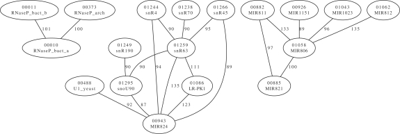
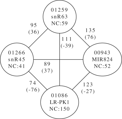
For our second example (Fig. 6), we have chosen a set of four family models. Each presents with not only a high Link score with regard to the others but also the scores are over the noise cutoff threshold by a large margin, too.

Fig. 6.

A high-scoring set of families, explicitly selected for the large difference to the noise cutoff value. Models 1259 and 943 score 135 bit on some input, which is at least 76 bit higher than the respective noise cutoff value. Notice, too, that not all pairs show such a behavior. Models 1086 and 943 have a high Link score with 123 bit, but at least the noise cutoff value is higher than this value (by 26 bit), making a hit less likely in one model. Some of the models were built using very few seed sequences and this seems to increase the chance of finding weak models.

These models show that high noise cutoff values are not necessarily enough. On the one hand there are indeed some 28 500 edges between families where the Link score is higher than both threshold values. In these cases one would reasonably argue to have found a homologue, even though the chance for a false positive does exist. One cannot, on the other hand, simply set the noise threshold to safe levels. This is because interesting sequences in the form of distant family members are likely to be found above the current noise threshold values.

The examples chosen for Figure 6 point out another problem with some of the models in the Rfam database. Models like RF00943 were created using only two seed sequences and five sequences in total. This is, of course, not a problem of Infernal but one of biological origin. As long as more members of the class have not been identified, the resulting models are a bit sketchy.

4 DISCUSSION

We have presented a polynomial-time algorithm that, for any two covariance models, returns a string that scores high in both models. Using this algorithm, several questions regarding RNA family models can be answered.

First, it is possible to determine if a model has high discriminative power against other models. This is important to avoid false positive results when searching for previously unknown new family members. The discriminative power can be quantified using the same measure as used in Infernal itself, thereby giving answers in a language, namely bit scores, that makes comparisons possible and easy.

Second, if a model shows overlap with another, it can be determined which regions of the model do actually show this behaviour. This is possible, as we not only return a score value, but other information, too. This includes the offending string, the respective secondary structures and a detailed score account.

Third, the algorithm is extendable. Borrowing ideas from Algebraic Dynamic Programming (Giegerich and Meyer, 2002), an optimization algebra can be anything that follows the dynamic programming constraints. Included are the CYK scoring algebra and the different information functions as well as an algebra product operation. Additional algebras require roughly a dozen lines of code.

Fourth, the MaxiMin, or Link score lends itself as a natural similarity score for RNA families. Closely related families, in terms of primary and secondary structure—not necessarily biological closeness, show a higher Link score than others. This requires further investigation to determine how much biological information can be extracted. Pure mathematics cannot answer which biological relation does actually exist.

In the case of prospective meta-families, we have two open research problems. One is to take a closer look at high-scoring families to determine their biological relationship. Are high scores an artifact of poorly designed families, or a case of an actual meta-family? The other problem became evident in the 1st example, where not all members of the RNaseP family scored high against each other. This suggests that meta-families cannot be modeled in Infernal directly, but how to adapt RNA family models in such a case remains open.

Researchers designing new families will also find value in the tool, as one can scan a new family model against existing ones to be more confident that one has indeed identified a new family and not an already existing one in disguise.

The Infernal Users Guide (Nawrocki et al., 2009b) mentions homology between family models as a reason for the existence of the different cutoff scores for noise, gathering and trusted. We think it is important to be able to determine, computationally, the importance of the cutoff scores when assigning new hits to families.

Another fact is that cutoff scores, like the models themselves, are set by the curators of the family. Our scoring scheme relies on the Infernal scoring algorithm itself. As numbers of models were created from very few seed sequences it is possible that the relevant cutoff scores are set too high to capture remote members. A cutoff score above the highest pair scores involving such a model could be of help while scanning new genomes for remote family members.

Finally, we have to acknowledge that Infernal uses the Inside-, not the CYK-algorithm to determine final scores. This can pose a problem in certain exceptional circumstances but these should be rare. Mathematically (cf. Nawrocki et al., 2009b), CYK = Prob(s, π|m), while Inside = Prob(s|m). The CYK algorithm gives the score for the single best alignment π of sequence s and model m while the Inside algorithm sums up over all possible alignments. This just means that we underestimate the final score, or said otherwise, the Inside scores for the Link sequence given the corresponding models will be even higher than the CYK scores.

Curated thresholds and Infernal 1.0:

The version change to Infernal 1.0 requires re-examination of all threshold values (cf. infernal.janelia.org). The next release of the Rfam database is expected to have done this, meaning that a comparison between (new) cutoff values and the scores calculated here is of current interest.

REFERENCES

- Bateman A, et al. The Pfam protein families database. Nucleic Acids Res. 2002;30:276–280. doi: 10.1093/nar/30.1.276. [DOI] [PMC free article] [PubMed] [Google Scholar]
- Dowell R, Eddy S. Evaluation of several lightweight stochastic context-free grammars for RNA secondary structure prediction. BMC Bioinformatics. 2004;5:71. doi: 10.1186/1471-2105-5-71. [DOI] [PMC free article] [PubMed] [Google Scholar]
- Durbin R, et al. Biological Sequence Analysis. Cambridge, New York: Cambridge University Press; 1998. [Google Scholar]
- Eddy S. HMMER: profile HMMs for protein sequence analysis. Bioinformatics. 1998;14:755–763. [Google Scholar]
- Eddy S, Durbin R. RNA sequence analysis using covariance models. Nucleic Acids Res. 1994;22:2079–2088. doi: 10.1093/nar/22.11.2079. [DOI] [PMC free article] [PubMed] [Google Scholar]
- Giegerich R, Höner zu Siederdissen C. Semantics and ambiguity of stochastic RNA family models. IEEE/ACM Trans. Comput. Biol. Bioinformatics. 2010;99 doi: 10.1109/TCBB.2010.12. Available at http://www.computer.org/portal/web/csdl/doi/10.1109/TCBB.2010.12. [DOI] [PubMed] [Google Scholar]
- Giegerich R, Meyer C. Algebraic Methodology And Software Technology. Vol. 2422. Berlin/Heidelberg: Springer; 2002. Algebraic Dynamic Programming; pp. 243–257. [Google Scholar]
- Griffiths-Jones S, et al. Rfam: An RNA family database. Nucleic Acids Res. 2003;31:439–441. doi: 10.1093/nar/gkg006. [DOI] [PMC free article] [PubMed] [Google Scholar]
- Mattick J, Makunin I. Non-coding RNA. Hum. Mol. Genet. 2006;15:R17–R29. doi: 10.1093/hmg/ddl046. [DOI] [PubMed] [Google Scholar]
- Nawrocki E, et al. Infernal 1.0: inference of RNA alignments. Bioinformatics. 2009a;25:1335–1337. doi: 10.1093/bioinformatics/btp157. [DOI] [PMC free article] [PubMed] [Google Scholar]
- Nawrocki E, et al. INFERNAL User Guide. 2009b [Google Scholar]
- Reeder J, Giegerich R. Consensus shapes: an alternative to the Sankoff algorithm for RNA consensus structure prediction. Bioinformatics. 2005;21:3516–3523. doi: 10.1093/bioinformatics/bti577. [DOI] [PubMed] [Google Scholar]