RactIP: fast and accurate prediction of RNA-RNA interaction using integer programming

Abstract

Motivation: Considerable attention has been focused on predicting RNA–RNA interaction since it is a key to identifying possible targets of non-coding small RNAs that regulate gene expression post-transcriptionally. A number of computational studies have so far been devoted to predicting joint secondary structures or binding sites under a specific class of interactions. In general, there is a trade-off between range of interaction type and efficiency of a prediction algorithm, and thus efficient computational methods for predicting comprehensive type of interaction are still awaited.

Results: We present RactIP, a fast and accurate prediction method for RNA–RNA interaction of general type using integer programming. RactIP can integrate approximate information on an ensemble of equilibrium joint structures into the objective function of integer programming using posterior internal and external base-paring probabilities. Experimental results on real interaction data show that prediction accuracy of RactIP is at least comparable to that of several state-of-the-art methods for RNA–RNA interaction prediction. Moreover, we demonstrate that RactIP can run incomparably faster than competitive methods for predicting joint secondary structures.

Availability: RactIP is implemented in C++, and the source code is available at http://www.ncrna.org/software/ractip/

Contact: ykato@kuicr.kyoto-u.ac.jp; satoken@k.u-tokyo.ac.jp

Supplementary information: Supplementary data are available at Bioinformatics online.

1 INTRODUCTION

Recent years have seen a renewal of interest in the biological roles of functional non-coding RNAs (ncRNAs). Modern studies have provided evidence that they can act as ubiquitous regulators in living cells (Eddy, 2001; Vogel and Wagner, 2007). A class of small ncRNAs downregulates gene expression post-transcriptionally via base-pairing with target mRNAs of the ncRNAs to inhibit the translation into the corresponding proteins. Eukaryotic microRNAs (miRNAs) and small interfering RNAs (siRNAs) are very short and have almost full sequence complementarity to their targets. On the other hand, several regulatory antisense RNAs have been found in bacterial chromosomes, which have relatively long sequences and interact with their target mRNAs in a more intricate manner (Brantl, 2002). This type of interaction comes from the fact that the genes encoding the antisense RNAs are located at loci different from those encoding their targets (i.e. trans-encoded antisense RNAs) (Wagner and Flärdh, 2002). In particular, kissing hairpin structures (see Fig. 1) caused by loop–loop interaction have been observed (Brunel et al., 2002). To help to understand the mechanism of RNA–RNA interaction further, as well as to identify target RNAs of specific ncRNAs, it is desirable to develop fast and accurate computational methods for predicting interacting RNA structures.

Fig. 1.

An example of RNA–RNA interaction containing two kissing hairpins. A broken line represents an internal base pair, and a black circle indicates a base that constitutes an external base pair (binding site).

RNA–RNA interaction prediction has so far been performed by several computational approaches, which can be roughly classified into four groups. The first group including UNAFold (Dimitrov and Zuker, 2004), RNAhybrid (Rehmsmeier et al., 2004) and RNAduplex from the Vienna RNA Package (Hofacker et al., 1994; Hofacker, 2003) disregards intramolecular bonds in both sequences and computes the minimum free energy (MFE) hybridization. They work out for short interacting RNAs but are impracticable for long sequences with intramolecular structures. The second group belongs to the category that uses the idea of concatenating two RNA sequences and considering them as a single strand so that the MFE structure of the resulting sequence can be computed. PairFold (Andronescu et al., 2005) and RNAcofold (Bernhart et al., 2006) adopt this procedure, but these methods cannot predict general type of interaction such as kissing hairpins. Other approaches such as RNAup (Mückstein et al., 2006), IntaRNA (Busch et al., 2008), inRNAs (Salari et al., 2010a) and bistaRNA (Poolsap et al., 2010) fall into the third group, which considers RNA–RNA interaction as the stepwise process of individual intramolecular foldings and their hybridization. RNAup and IntaRNA can predict only one binding site, whereas inRNAs and bistaRNA can predict multiple binding sites. The final group aims at predicting the MFE joint secondary structure or computing the interaction partition function under the comprehensive type of interaction. IRIS (Pervouchine, 2004), inteRNA (Alkan et al., 2006), RIG (Kato et al., 2009), piRNA (Chitsaz et al., 2009), rip (Huang et al., 2009, 2010) and also inRNAs (Salari et al., 2010a) are listed as this category. These methods impose natural constraints on the joint structure such that there are no internal pseudoknots, crossing interactions and zigzags (Alkan et al., 2006; Chitsaz et al., 2009). Note that Alkan et al. suggested that these constraints are satisfied by all examples of complex RNA–RNA interactions in the literature. In this sense, we can consider the class of joint structures satisfying those constraints the most general type of interaction. Although the final group can cover wider class of interacting structures simultaneously, their computational costs could be prohibitively expensive for long sequences.

Prediction of interacting RNA structure can be considered as a kind of optimization problem in a sense that we seek to minimize the free energy of the joint structure or maximize a score such as an interaction probability under the possible topology of the interacting structure. Various problems presented in bioinformatics have been formulated as mathematical programming problems, where the objective function is minimized or maximized under some constraints. Recently, Bauer et al. (2007) presented LARA that implements an integer programming-based method for multiple structural alignment of RNA sequences. To reduce the computational cost of the structural alignment, they simplified the mathematical structure of the integer programming (IP) formulation, eliminating information on the topology of secondary structure from the constraints and integrating the structural information into the objective function, as well as using the Lagrangian relaxation. In general, IP problems are known to be NP-hard, but use of IP formulation fascinates us due to its strong and flexible descriptive power to model a large number of combinatorial optimization problems.

Motivated in part by Bauer et al.'s work, we present a novel method called RactIP, RNA–RNA interACTion prediction using Integer Programming. In our IP formulation, the objective function, which is to be maximized, is defined as the sum of scores with respect to internal and external base pairs of two interacting RNAs. In particular, we make use of posterior probabilities such as base-pairing probabilities and hybridization probabilities for scores of internal pairs and those of external pairs, respectively, to incorporate further structural information into the objective function as in the case of LARA (Bauer et al., 2007). It is to be noted that use of such posterior probabilities enables the method to take account of an ensemble of equilibrium structures approximately, which will lead to improve expected accuracy. We introduce a threshold cut technique to solve the IP problem efficiently, which is shown to be reasonable from the viewpoint of maximizing expected accuracy. By virtue of this technique, RactIP achieves considerably short run-time despite the computational hardness of IP. We demonstrate the prediction performance of RactIP on a set of known interacting RNA pairs both for joint structure prediction and binding site prediction, making a comparison with several state-of-the-art methods. Advantages of RactIP are summarized as follows:

• As for joint secondary structure prediction under the most general type of interaction, RactIP can run overwhelmingly faster than competitive prediction methods with O(n⁶) time complexities, where n is the length of the longer input sequence. In fact, experimental results reveal that computation time of RactIP is an order of magnitude shorter than that of inRNAs (the joint structure prediction model) (Salari et al., 2010a), inteRNA (the Loop Model) (Alkan et al., 2006) and rip (Huang et al., 2009, 2010). Recently, Salari et al. (2010b) proposed a sparsified dynamic programming algorithm whose time complexity is O(n⁵) on average. To the best of the authors' knowledge, RactIP is the fastest method for predicting both internal structures and binding sites simultaneously on condition of the comprehensive class of interactions.

• RactIP is comparable in accuracy to inRNAs (the joint structure prediction model) and outperforms inteRNA and rip for joint structure prediction. From the viewpoint of binding site prediction that disregards (predicted) internal base pairs, accuracy of RactIP is as good as that of inRNAs (the binding site prediction model) and better than that of IntaRNA (Busch et al., 2008).

• The mathematical model of RactIP is compact. In particular, the IP objective function fit in well with the sum of the posterior probabilities that consider many complex loop energies necessary to achieve prediction of good quality.

• The IP-based method is flexible and extensible. Compared with other computational approaches, it is easy to change the model to cope with a desired class of secondary structures simply by adding or removing appropriate constraints. In our model, we employ additional constraints to represent stacking base pairs, which is expected to improve prediction accuracy.

The rest of the article is organized as follows. Section 2 describes our prediction model RactIP in detail after providing several preliminaries to grasp it. We show experimental results of interaction prediction and discuss them in Sections 3 and 4, respectively. Section 5 concludes the article.

2 METHODS

We propose a new method RactIP for RNA–RNA interaction prediction using IP. RactIP executes the following two steps when two RNA sequences are given:

1. compute the score matrices of the IP objective function for internal and external base pairs;

2. solve the IP problem to predict the optimal joint secondary structure.

It should be noted that the program RactIP actually solves the IP problem using libraries of a high-performance solver (see Section 3 for details).

2.1 Scoring functions for predicting RNA–RNA interaction

Let Σ = {A, C, G, U} and Σ^* denote the set of all finite RNA sequences consisting of bases in Σ. For a sequence a ∈ Σ^*, let |a| denote the number of symbols appearing in a, which is called the length of a. For 1 ≤ i < j ≤ |a|, we let a[i..j] denote a sequence a_ia_i+1···a_j ∈ Σ^*.

Let 𝒮(a) be a space of all possible secondary structures of a sequence a ∈ Σ^*. An element x ∈ 𝒮(a) is represented as a |a|² binary-valued triangular matrix x = (x_ij)_i<j, where x_ij = 1 means that bases a_i and a_j form a base pair. We denote by P(x ∣ a) a probability distribution over 𝒮(a). Let ℋ(a, b) be a space of all possible hybridized structures between a, b ∈ Σ^*, which considers no secondary structures of a and b. An element z ∈ ℋ(a, b) is represented as a |a| × |b| binary-valued matrix z = (z_ij), where z_ij = 1 means that the base a_i interacts with the base b_j. We denote by P(z ∣ a, b) a probability distribution over ℋ(a, b). Let 𝒥𝒮(a, b) be a space of the joint secondary structures of a and b that considers both the secondary structures of a and b and the hybridized structures between a and b. In other words, 𝒥𝒮(a, b) is a subset of 𝒮(a) × 𝒮(b) × ℋ(a, b). We denote by P(σ ∣ a, b) a probability distribution over 𝒥𝒮(a, b), where σ = (x, y, z) ∈ 𝒥𝒮(a, b) such that x ∈ 𝒮(a), y ∈ 𝒮(b) and z ∈ ℋ(a, b). We assume that each base can be paired with at most one base regardless of whether the base pair is formed inside or outside the sequence, and internal pseudoknots and crossing interactions (external pseudoknots) are disallowed.

We now define the problem of predicting RNA-RNA interaction as follows:

Definition 1 —

(RNA–RNA interaction prediction). Given two RNA sequences a = a[1..n] ∈ Σ^* (5′–3′ direction) and b = b[1..m] ∈ Σ^* (3′–5′ direction), predict a joint secondary structure σ ∈ 𝒥𝒮(a, b).

To tackle this problem, we first define the gain function for the true joint structure σ = (x, y, z) and a predicted joint structure as

(1)

where

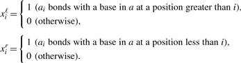
Here, I(condition) is the indicator function that takes a value of 1 or 0 depending on whether the condition is true or false, γ_s and γ_h are weight parameters for base pairs, and α is a balancing parameter between internal base pairs and external base pairs. The gain function (1) is equal to the weighted sum of the number of true positives and the number of true negatives of base pairs. In order to maximize the expected number of true predictions, we find a joint secondary structure that maximizes the expectation of the gain function (1) with respect to an ensemble of all possible joint secondary structures under a given posterior distribution:

(2)

For the posterior distribution P(σ ∣ a, b) over a space of joint secondary structures, we can employ the piRNA model (Chitsaz et al., 2009) and the rip model (Huang et al., 2009, 2010). However, these exact models are impractical since O(n⁶) time and O(n⁴) space are required where n is the length of the longer RNA sequence. Therefore, we approximate the posterior distribution over a space of joint secondary structures by its factorization:

(3)

for σ = (x, y, z) (Fig. 2). As a result, the expected gain (2) can be replaced by

(4)

where C is a constant independent of , p^(a)_ij = ∑_x∈𝒮(a)I(x_ij = 1)P(x∣a) is a base-pairing probability that the base a_i is paired with a_j, and q_ij = ∑_z∈ℋ(a,b)I(z_ij = 1)P(z∣a, b) is a hybridization probability that the base a_i interacts with the base b_j (see Supplementary Material for the derivation). Finally, we find a joint structure that maximizes the approximate estimator (4). We should notice that maximizing the approximate estimator (4) is equivalent to maximizing the sum of: (i) the sum of the base-pairing probabilities p^(a)_ij larger than θ_s = 1/(γ_s+1); (ii) the sum of the base-pairing probabilities p^(b)_ij larger than θ_s; and (iii) the sum of the hybridization probabilities q_ij larger than θ_h = 1/(γ_h+1). This means that there is no need to consider the base pairs whose posterior probabilities are at most the predefined thresholds θ_s and θ_h so that the search space for the optimal structure can be reduced. This threshold cut technique makes our method run much faster.

Fig. 2.

An illustration of the factorization [Equation (3)] of the posterior probability P(σ ∣ a, b) of a joint structure σ. A broken line shows an internal or external base pair.

2.2 IP model

2.2.1 Definition of IP

Integer (linear) programming, which is one of the mathematical programming methods, seeks to maximize/minimize a linear function called objective function subject to linear equality and/or inequality constraints. The most important constraint of IP is that specified variables must take integral values. An IP problem where all variables are non-negative integers can be described as follows:

where a_ij, b_i, c_j ∈ ℝ and x_j is a variable defined over a set ℤ₊ of non-negative integers.

2.2.2 Formulation for RNA–RNA interaction prediction

We use the entries of the binary-valued triangular matrices x = (x_ij)_i<j ∈ 𝒮(a), y = (y_ij)_i<j ∈ 𝒮(b) and z = (z_ij) ∈ ℋ(a, b) defined in Section 2.1 as the fundamental IP variables for describing internal and external base pairs. Figure 3 indicates a simple kissing hairpin structure by setting these variables as x_ij = 1, y_i′j′ = 1 and z_kl = 1 where i < k < j and i′ < l < j′. With these variables, we can formulate an IP problem for joint secondary structure prediction as follows:

(5)

(6)

(7)

(8)

(9)

(10)

where p_ij^(a), p_ij^(b) and q_ij denote the base-pairing probabilities and the hybridization probability defined in Section 2.1, respectively, and α ∈ (0, 1) is a parameter that regulates the proportion of hybridization in the predicted structure. Recall that values of all variables must be either 0 or 1.

Fig. 3.

An illustration of variables used in the IP formulation. This variable setting enables the model to represent a kissing hairpin.

Here, let us look more carefully into each equation of the above IP formulation. The objective function (5) shows an instantiation of the approximate estimator (4) using the base-pairing probabilities and hybridization probabilities. Note that the third term describing sum of scores of external base pairs is multiplied by a positive weight parameter α. As suggested by Alkan et al. (2006), we set α ∈ (0, 1) so that external base pairs are less likely to be formed than internal ones. In this study, we fix α = 0.5, that is, external base pairs contribute to the objective function by half compared with internal base pairs. Constraints (6) and (7) mean that each base can be paired with at most one base regardless of whether the base pair is formed inside or outside the sequence (Fig. 4a). Internal pseudoknots and crossing interactions are prohibited by constraints (8), (9) and the constraint (10), respectively (Fig. 4b and c).

Fig. 4.

An illustration of several constraints of the IP formulation. In each of the three diagrams, at most one variable shown by a broken (curved) line can take a value 1.

To solve the IP problem, we employ the threshold cut technique where we exclude the IP variables in advance representing internal and external base pairs whose posterior probabilities are not exceeding θ_s and θ_h, respectively, defined in Section 2.1, before computing the optimal solution. As described in Section 2.1, this threshold cut is derived from the viewpoint of maximizing expected accuracy of joint structure prediction.

2.2.3 Incorporating stacked pairing constraints

It is widely accepted that base pairs in stable RNA structures are likely to appear in a stacked form rather than an isolated one. Following the IP formulation for predicting secondary structure of a single RNA sequence proposed by Poolsap et al. (2009), we define further variables for promoting stacking base pairs as follows:

In the IP formulation, we describe the definitions of x_i^ℓ and x_i^r as

We should notice that the following ingenious constraints containing linear combinations of these variables actually play a role in yielding stacking base pairs:

(11)

(12)

These constraints guarantee that if a base a_i is paired with another one, the base(s) adjacent to a_i must also form a base pair (Fig. 5). The rest of the variable definitions with respect to the sequence b and interaction part, and related constraints, are similarly represented in the IP formulation.

Fig. 5.

An illustration of stacked pairing constraints of the IP formulation.

3 RESULTS

3.1 Implementation

Our method was implemented as a program called RactIP, which uses Gurobi optimizer 2.0 (http://gurobi.com/) for solving the IP problem. We employed the CONTRAfold model (Do et al., 2006) for the probability distribution of RNA secondary structures and the RNAduplex model for the probability distribution of hybridization of two RNA sequences. CONTRAfold, based on a machine-learning algorithm, is one of the most accurate programs for predicting RNA secondary structures. We utilized part of CONTRAfold to calculate base-pairing probabilities p_ij^(a) and p_ij^(b). RNAduplex is a program from the Vienna RNA package (Hofacker et al., 1994; Hofacker, 2003) for computing the MFE structure of hybridization of two RNA sequences. We modified the code of RNAduplex to calculate hybridization probabilities q_ij instead of the MFE structures, designing a forward-backward-like algorithm. The source code of RactIP is freely available at http://www.ncrna.org/software/ractip/.

3.2 Data

In our experiments, we used two datasets of RNA–RNA interactions. The first set comprises five pairs of RNA sequences with their joint secondary structures including kissing hairpins, which was used by Kato et al. (2009). We made use of this set to evaluate the performance of joint secondary structure prediction. The second set contains 18 sRNA–target pairs with their binding sites, which was used by Busch et al. (2008). All of the two datasets (i.e. 23 pairs of interacting RNAs) were used to assess the performance of binding site prediction.

3.3 Joint structure prediction

We first conducted experiments in joint secondary structure prediction on the dataset compiled by Kato et al. (2009). The performance was evaluated by sensitivity and positive predictive value (PPV) defined as follows:

where TP is the number of correctly predicted base pairs, FN is the number of base pairs in the true structure that were not predicted, and FP is the number of incorrectly predicted base pairs. We also used F-measure as the balanced measure between sensitivity and PPV, which is defined as the harmonic mean of them:

We compared our method RactIP with two state-of-the-art methods: inRNAs (the exact model for joint structure prediction) (Salari et al., 2010a) and inteRNA (Alkan et al., 2006). The accuracy of inRNAs is extracted from their literature. In order to calculate the accuracy of inteRNA, we computed the joint structure of each pair in the dataset by using the inteRNA Web server with default settings (Aksay et al., 2007) (http://compbio.cs.sfu.ca/taverna/interna/).

Table 1 shows the results of joint structure prediction using our approach and two existing methods. As can be seen, RactIP outperforms inteRNA and is comparable to inRNAs. It should be noted that computation time of RactIP includes both the pre-processing step to calculate posterior pairing probabilities and the one to solve the IP problem. We did not compare the running time strictly between the three methods due to difficulty in their availability. However, we would like to remark that Salari et al. (2010a) reported in their literature that inRNAs runs for ∼4000 s on Sun Fire X4600 2.6 GHz with 64 GB memory to predict the joint structures of CopA–CopT and IncRNA₅₄-RepZ. Meanwhile, RactIP consumes only 0.13 s and 0.10 s to predict the joint structures of CopA-CopT and IncRNA₅₄-RepZ, respectively, on Mac OS X 10.6 running on Intel Core 2 Duo 2.13 GHz with 2 GB memory.

Table 1.

Comparison with competitive methods for joint structure prediction

Antisense-target	No. of sites	Sensitivity			PPV			F-measure			Time (s)
		RactIP	inRNAs	inteRNA	RactIP	inRNAs	inteRNA	RactIP	inRNAs	inteRNA	RactIP
CopA-CopT	2	1.000	1.000	0.731	0.754	0.846	0.655	0.860	0.917	0.691	0.13
DIS-DIS	1	1.000	1.000	1.000	1.000	1.000	1.000	1.000	1.000	1.000	0.05
IncRNA54-RepZ	1	0.813	0.875	0.958	0.736	0.792	0.836	0.772	0.831	0.893	0.10
R1inv-R2inv	1	1.000	0.900	0.800	1.000	0.900	0.889	1.000	0.900	0.842	0.03
Tar-Tar*	1	1.000	1.000	1.000	0.875	0.875	0.875	0.933	0.933	0.933	0.03
Average		0.963	0.955	0.898	0.873	0.883	0.851	0.913	0.916	0.872

The five RNA–RNA interaction pairs were predicted by RactIP, inRNAs (the joint structure prediction model) (Salari et al., 2010a) and inteRNA (the Loop Model) (Aksay et al., 2007; Alkan et al., 2006). In the table, No. of sites represents the number of binding sites. We set the parameters for RactIP as α=0.5, θ_s=0.5 and θ_h=0.2. Running time of RactIP was measured on Mac OS X 10.6 running Intel Core 2 Duo 2.13 GHz with 2 GB memory. Note that computation time of inRNAs is reported to be at most 4000 s for long sequences on Sun Fire X4600 2.6 GHz with 64 GB memory (Salari et al., 2010a).

3.4 Binding site prediction

In the second experiment, we assessed the performance of predicting binding sites on the dataset reported by Kato et al. (2009) and Busch et al. (2008). The accuracy was measured by sensitivity, PPV and F-measure such that only external base pairs are considered. Table 2 shows the results of prediction by our program RactIP, inRNAs (the heuristic model for binding site prediction) (Salari et al., 2010a) extracted from their literature, and IntaRNA (Busch et al., 2008) with default settings, indicating that our method is more accurate or comparable as compared with the existing methods. It is worth noting that RactIP has no restriction on the number of accessible regions to predict, whereas IntaRNA and inRNAs can consider only one or two accessible regions that are putative binding sites.

Table 2.

Comparison with competitive methods for binding site prediction

Antisense-target	No. of sites	Sensitivity			PPV			F-measure			Time (s)
		RactIP	inRNAs	IntaRNA	RactIP	inRNAs	IntaRNA	RactIP	inRNAs	IntaRNA	RactIP	inRNAs	IntaRNA
CopA-CopT	2	0.815	0.889	1.000	0.579	0.828	0.391	0.677	0.857	0.562	0.14	0.21	0.14
DIS-DIS	1	1.000	1.000	1.000	1.000	1.000	1.000	1.000	1.000	1.000	0.04	0.03	0.04
IncRNA54-RepZ	1	0.750	1.000	0.738	0.783	0.889	0.850	0.766	0.941	0.790	0.10	2.56	0.11
R1inv-R2inv	1	1.000	1.000	1.000	1.000	0.778	1.000	1.000	0.875	1.000	0.03	0.03	0.02
Tar-Tar*	1	1.000	1.000	1.000	0.833	0.833	0.833	0.909	0.909	0.909	0.02	0.03	0.03
DsrA-RpoS	1	0.654	0.808	0.808	0.739	0.778	0.778	0.694	0.793	0.793	0.06	6.80	0.05
GcvB-argT	1	0.950	0.950	0.950	1.000	0.864	0.950	0.974	0.905	0.950	0.04	8.07	0.03
GcvB-dppA	1	0.941	1.000	1.000	0.593	0.850	0.586	0.727	0.919	0.739	0.05	5.59	0.04
GcvB-gltI	1	1.000	0.750	0.000	1.000	0.500	0.000	1.000	0.600	0.000	0.05	2.74	0.04
GcvB-livJ	1	0.955	0.634	0.955	0.955	0.824	0.955	0.955	0.717	0.955	0.04	6.10	0.04
GcvB-livK	1	0.958	0.540	0.542	0.958	0.570	0.565	0.958	0.555	0.553	0.04	3.24	0.03
GcvB-oppA	1	1.000	1.000	1.000	1.000	0.733	0.957	1.000	0.846	0.978	0.05	8.23	0.04
GcvB-STM4351	1	0.880	0.760	0.760	1.000	1.000	0.905	0.936	0.864	0.826	0.04	2.59	0.04
IstR-tisAB	1	0.778	0.722	0.879	1.000	1.000	0.960	0.875	0.839	0.918	0.05	8.24	0.05
MicA-ompA	1	0.875	1.000	1.000	0.875	1.000	1.000	0.875	1.000	1.000	0.32	3.29	0.04
MicA-lamB	1	0.565	1.000	1.000	0.867	1.000	0.821	0.684	1.000	0.902	0.08	5.38	0.08
MicC-ompC	1	0.727	1.000	1.000	0.889	1.000	0.537	0.800	1.000	0.699	0.07	8.11	0.06
MicF-ompF	1	0.833	0.960	0.960	0.769	0.960	0.960	0.800	0.960	0.960	0.73	17.82	0.83
OxyS-fhlA	2	0.563	0.813	0.500	0.818	1.000	1.000	0.667	0.897	0.667	0.32	0.21	0.39
RyhB-sdhD	1	0.824	0.618	0.588	0.824	0.955	1.000	0.824	0.750	0.741	0.07	7.74	0.06
RyhB-sodB	1	1.000	1.000	1.000	0.391	1.000	0.818	0.563	1.000	0.900	0.19	3.23	0.21
SgrS-ptsG	1	0.739	0.566	0.739	1.000	0.765	1.000	0.850	0.651	0.850	0.06	12.07	0.05
Spot42-galK	1	0.682	0.432	0.409	0.698	0.760	0.643	0.690	0.551	0.500	0.13	5.94	0.13
Average		0.847	0.845	0.819	0.851	0.865	0.805	0.836	0.845	0.791

The 23 RNA–RNA interaction pairs were predicted by RactIP, inRNAs (the binding site prediction model) (Salari et al., 2010a) and IntaRNA (Busch et al., 2008). We set the parameters for RactIP as α=0.5, θ_s=0.3 and θ_h=0.5. Running time of RactIP and IntaRNA was measured on Mac OS X 10.6 running on Intel Core 2 Duo 2.13 GHz with 2 GB memory. Computation time of inRNAs measured on Intel Core 2 Duo 2.53 GHz with 4 GB memory was given by R. Salari (personal communication).

3.5 Time and accuracy trade-off by approximation

To confirm the effectiveness of approximating the joint posterior distribution by its factorization, we compared running time and prediction accuracy of the factorized model that we proposed with those of the naïve model by rip (Huang et al., 2009, 2010). rip calculates exact base-pairing probabilities of internal base pairs and external base pairs by taking O(n⁶) time and O(n⁴) space where n is the length of the longer sequence. We compared RactIP with rip, which samples joint structures from internal and external base-pairing probabilities, and RactIP combined with rip, in which internal and external base-pairing probabilities calculated by rip were used in the IP [see Equation (5)] instead of factorized ones. Note that rip failed to calculate base-pairing probabilities for the CopA–CopT pair since their length might be too long for rip. As shown in Table 3, our approximation by factorization is significantly faster than the naïve calculation of base-pairing probabilities, though the accuracy of our approximation dropped slightly. The results indicate that our method can be applicable to joint secondary structure prediction for long sequences.

Table 3.

Comparison of accuracy and running time for joint structure prediction

Antisense target	Sensitivity			PPV			F-measure			Time
	RactIP	rip	rip+RactIP	RactIP	rip	rip+RactIP	RactIP	rip	rip+RactIP	RactIP (s)	rip
DIS-DIS	1.000	0.500	0.500	1.000	0.500	0.500	1.000	0.500	0.500	0.05	19 m 40 s
IncRNA54-RepZ	0.813	0.562	1.000	0.736	0.500	0.889	0.772	0.529	0.941	0.10	860 m
R1inv-R2inv	1.000	0.900	1.000	1.000	0.900	1.000	1.000	0.900	1.000	0.03	37 s
Tar-Tar*	1.000	1.000	1.000	0.875	0.875	0.875	0.933	0.933	0.933	0.03	9.5 s

The four RNA–RNA interaction pairs were predicted by RactIP, rip (Huang et al., 2009, 2010) and RactIP with base-pairing probabilities calculated by rip (rip+RactIP). We set the parameters for RactIP as α=0.5, θ_s=0.5 and θ_h=0.2. Running time of RactIP was measured on Mac OS X 10.6 running on Intel Core 2 Duo 2.13 GHz with 2 GB memory. Computation time of rip was measured on linux kernel 2.6.30 running on Intel Xeon 3.33 GHz with 32 GB memory.

4 DISCUSSION

We employed the threshold cut technique to reduce the search space for the optimal joint secondary structure, which makes RactIP run much faster than existing state-of-the-art algorithms for joint structure prediction. Let us stress again that there is a close relation between the threshold cut and maximizing expected accuracy. The scoring scheme of RactIP can be regarded as the generalized centroid estimator (Hamada et al., 2009) since the gain function (1) with γ_s = γ_h and α = 1 corresponds to the γ-centroid estimator. As described in Section 2.1, the thresholds correspond to the weights for base pairs in Equation (1), which control the balance between the expected number of true positives and that of true negatives. This means that an appropriate choice of the thresholds will improve the balanced accuracy such as F-measure. See Supplementary Material for more details.

In the experiments, we used the combination of the parameters derived from the machine-learning model and the ones from the thermodynamic model to implement the scores of the RactIP objective function. It is possible to adopt such a hybrid scoring scheme due to the factorization of the posterior probability of a joint structure shown in Equation (3). In fact, prediction accuracy decreased when adopting the identical scoring scheme (e.g. the CONTRAfold model is used to derive both base-pairing probabilities and hybridization probabilities). The main reason will be that the machine-learning model (CONTRAfold) specializes in predicting internal secondary structures, whereas the thermodynamic model (RNAduplex) aims at predicting hybridized structures. Therefore, the approximation enables us to select good models separately and integrate them into the prediction model.

The results shown in Table 2 tell us that RactIP performs worse than inRNAs and is not significantly better than IntaRNA on CopA–CopT and OxyS–fhlA pairs with two binding sites. One reason is that lack of interaction data with multiple binding sites makes our method fail to optimize appropriately. Nevertheless, we would like to emphasize again that RactIP can deal with complex interactions with more than one binding site in the framework of the integer programming formulation. As our future work, optimizing hybridization scores appropriately is necessary to improve prediction performance on the data with multiple binding sites.

5 CONCLUSION

We proposed RactIP, a novel method for predicting RNA–RNA interaction of general type using IP. In our approach, the threshold cut technique was adopted to reduce the complexity of the solution space of the IP problem, which also leads to maximizing expected accuracy. Experimental results on real interaction data demonstrated that prediction accuracy of RactIP is at least comparable to that of several state-of-the-art methods for joint structure prediction and binding site prediction. Although it is difficult to evaluate theoretically the time complexity of our IP-based approach, experimental validations revealed that RactIP can run much faster than competitive methods for predicting joint secondary structures. This is an important fact to stress since RactIP is expected to improve prediction performance in unknown target search in long genomes by predicting respective intramolecular structures as well as intermolecular binding sites in practical time. For this purpose, we should also show that RactIP can discriminate between targets and non-targets, which is left as our future work. RactIP not only achieved success in RNA–RNA interaction prediction but also showed further possibility of applying the fast IP-based method with threshold cut to other biologically important problems, which are worthwhile and challenging tasks.

REFERENCES

- Aksay C, et al. taveRNA: a web suite for RNA algorithms and applications. Nucleic Acids Res. 2007;35:W325–W329. doi: 10.1093/nar/gkm303. [DOI] [PMC free article] [PubMed] [Google Scholar]
- Alkan C, et al. RNA-RNA interaction prediction and antisense RNA target search. J. Comput. Biol. 2006;13:267–282. doi: 10.1089/cmb.2006.13.267. [DOI] [PubMed] [Google Scholar]
- Andronescu M, et al. Secondary structure prediction of interacting RNA molecules. J. Mol. Biol. 2005;345:987–1001. doi: 10.1016/j.jmb.2004.10.082. [DOI] [PubMed] [Google Scholar]
- Bauer M, et al. Accurate multiple sequence-structure alignment of RNA sequences using combinatorial optimization. BMC Bioinformatics. 2007;8:271. doi: 10.1186/1471-2105-8-271. [DOI] [PMC free article] [PubMed] [Google Scholar]
- Bernhart SH, et al. Partition function and base pairing probabilities of RNA heterodimers. Algorithms Mol. Biol. 2006;1:3. doi: 10.1186/1748-7188-1-3. [DOI] [PMC free article] [PubMed] [Google Scholar]
- Brantl S. Antisense-RNA regulation and RNA interference. Biochim. Biophys. Acta. 2002;1575:15–25. doi: 10.1016/s0167-4781(02)00280-4. [DOI] [PubMed] [Google Scholar]
- Brunel C, et al. RNA loop-loop interactions as dynamic functional motifs. Biochimie. 2002;84:925–944. doi: 10.1016/s0300-9084(02)01401-3. [DOI] [PubMed] [Google Scholar]
- Busch A, et al. IntaRNA: efficient prediction of bacterial sRNA targets incorporating target site accessibility and seed regions. Bioinformatics. 2008;24:2849–2856. doi: 10.1093/bioinformatics/btn544. [DOI] [PMC free article] [PubMed] [Google Scholar]
- Chitsaz H, et al. A partition function algorithm for interacting nucleic acid strands. Bioinformatics. 2009;25:i365–i373. doi: 10.1093/bioinformatics/btp212. [DOI] [PMC free article] [PubMed] [Google Scholar]
- Dimitrov RA, Zuker M. Prediction of hybridization and melting for double-stranded nucleic acids. Biophys. J. 2004;87:215–226. doi: 10.1529/biophysj.103.020743. [DOI] [PMC free article] [PubMed] [Google Scholar]
- Do CB, et al. CONTRAfold: RNA secondary structure prediction without physics-based models. Bioinformatics. 2006;22:e90–e98. doi: 10.1093/bioinformatics/btl246. [DOI] [PubMed] [Google Scholar]
- Eddy SR. Non-coding RNA genes and the modern RNA world. Nat. Rev. Genet. 2001;2:919–929. doi: 10.1038/35103511. [DOI] [PubMed] [Google Scholar]
- Hamada M, et al. Prediction of RNA secondary structure using generalized centroid estimators. Bioinformatics. 2009;25:465–473. doi: 10.1093/bioinformatics/btn601. [DOI] [PubMed] [Google Scholar]
- Hofacker IL, et al. Fast folding and comparison of RNA secondary structures. Monatsh. Chem. 1994;125:167–188. [Google Scholar]
- Hofacker IL. Vienna RNA secondary structure server. Nucleic Acids Res. 2003;31:3429–3431. doi: 10.1093/nar/gkg599. [DOI] [PMC free article] [PubMed] [Google Scholar]
- Huang FWD, et al. Partition function and base pairing probabilities for RNA-RNA interaction prediction. Bioinformatics. 2009;25:2646–2654. doi: 10.1093/bioinformatics/btp481. [DOI] [PubMed] [Google Scholar]
- Huang FWD, et al. Target prediction and a statistical sampling algorithm for RNA-RNA interaction. Bioinformatics. 2010;26:175–181. doi: 10.1093/bioinformatics/btp635. [DOI] [PMC free article] [PubMed] [Google Scholar]
- Kato Y, et al. A grammatical approach to RNA-RNA interaction prediction. Pattern Recognit. 2009;42:531–538. [Google Scholar]
- Mückstein U, et al. Thermodynamics of RNA-RNA binding. Bioinformatics. 2006;22:1177–1182. doi: 10.1093/bioinformatics/btl024. [DOI] [PubMed] [Google Scholar]
- Pervouchine DD. IRIS: intermolecular RNA interaction search. Genome Inform. 2004;15:92–101. [PubMed] [Google Scholar]
- Poolsap U, et al. Prediction of RNA secondary structure with pseudoknots using integer programming. BMC Bioinformatics. 2009;10(Suppl. 1):S38. doi: 10.1186/1471-2105-10-S1-S38. [DOI] [PMC free article] [PubMed] [Google Scholar]
- Poolsap U, et al. Dynamic programming algorithms for RNA structure prediction with binding sites. Proc. Pac. Symp. Biocomput. 2010;15:98–107. doi: 10.1142/9789814295291_0012. [DOI] [PubMed] [Google Scholar]
- Rehmsmeier M, et al. Fast and effective prediction of microRNA/target duplexes. RNA. 2004;10:1507–1517. doi: 10.1261/rna.5248604. [DOI] [PMC free article] [PubMed] [Google Scholar]
- Salari R, et al. Fast prediction of RNA-RNA interaction. Algorithms Mol. Biol. 2010a;5:5. doi: 10.1186/1748-7188-5-5. [DOI] [PMC free article] [PubMed] [Google Scholar]
- Salari R, et al. Time and space efficient RNA-RNA interaction prediction via sparse folding. Lect. Notes Bioinformatics. 2010b;6044:473–490. [Google Scholar]
- Vogel J, Wagner EGH. Target identification of small noncoding RNAs in bacteria. Curr. Opin. Microbiol. 2007;10:262–270. doi: 10.1016/j.mib.2007.06.001. [DOI] [PubMed] [Google Scholar]
- Wagner EGH, Flärdh K. Antisense RNAs everywhere? Trends Genet. 2002;18:223–226. doi: 10.1016/s0168-9525(02)02658-6. [DOI] [PubMed] [Google Scholar]
Associated Data
This section collects any data citations, data availability statements, or supplementary materials included in this article.