

Abstract
Motivation: Intrinsically disordered proteins play a crucial role in numerous regulatory processes. Their abundance and ubiquity combined with a relatively low quantity of their annotations motivate research toward the development of computational models that predict disordered regions from protein sequences. Although the prediction quality of these methods continues to rise, novel and improved predictors are urgently needed.
Results: We propose a novel method, named MFDp (Multilayered Fusion-based Disorder predictor), that aims to improve over the current disorder predictors. MFDp is as an ensemble of 3 Support Vector Machines specialized for the prediction of short, long and generic disordered regions. It combines three complementary disorder predictors, sequence, sequence profiles, predicted secondary structure, solvent accessibility, backbone dihedral torsion angles, residue flexibility and B-factors. Our method utilizes a custom-designed set of features that are based on raw predictions and aggregated raw values and recognizes various types of disorder. The MFDp is compared at the residue level on two datasets against eight recent disorder predictors and top-performing methods from the most recent CASP8 experiment. In spite of using training chains with ≤25% similarity to the test sequences, our method consistently and significantly outperforms the other methods based on the MCC index. The MFDp outperforms modern disorder predictors for the binary disorder assignment and provides competitive real-valued predictions. The MFDp's outputs are also shown to outperform the other methods in the identification of proteins with long disordered regions.
Availability: http://biomine.ece.ualberta.ca/MFDp.html
Supplementary information: Supplementary data are available at Bioinformatics online.
Contact: lkurgan@ece.ualberta.ca
1 INTRODUCTION
The intrinsically disordered proteins (IDPs), also referred to as unstructured proteins, lack stable tertiary structure under physiological conditions in vitro. The IDPs play a crucial role in transcriptional regulation, translation and cellular signal transduction (Dunker et al., 2008). Their prevalence was also implicated in various human disorders including the neuro-degenerative diseases such as Huntington, Parkinson's and Alzheimer's disease (Raychaudhuri et al., 2009). However, the functional role of IDPs is not as well understood when compared with the well-packed proteins. Importantly, the annotations of the disorder lag behind the rapidly accumulating number of known protein chains. To compare, the curated DisProt database (Sickmeier et al., 2007) includes little over 500 chains, the PDB database (Berman et al., 2000) that allows finding unstructured segments in the solved tertiary structures (which are assumed to be equivalent to disordered segments) includes ∼ 58 000 proteins, while the overall number of known protein chains is >9 million. The disorder is frequently observed in regions with low-sequence complexity and with low content of hydrophobic amino acids, which would often form a core of a folded globular protein (Dyson and Wright, 2005; Uversky et al., 2000). These and other sequence characteristics can be used to differentiate between disordered and ordered regions, which in turn implies that disorder is predictable from the sequence. The past decade observed development of a number of computational models for the prediction of the disordered regions. These methods allow for high-throughput annotations of protein chains which provide a viable solution to close the annotation gap. These predictors could be categorized into four groups: (i) methods based on relative propensity of amino acids to form disorder/ordered regions which include GlobPlot (Linding et al., 2003), IUPred (Dosztányi et al., 2005), FoldIndex (Prilusky et al., 2005) and Ucon (Schlessinger et al., 2007a); (ii) methods built utilizing machine-learning classifiers, such as DISpro (Hecker et al., 2008), DISOPRED (Jones and Ward, 2003) DISOPRED2 (Ward et al., 2004), PrDOS (Ishida and Kinoshita, 2007), POODLE-S (Shimizu et al., 2007a), POODLE-L (Hirose et al., 2007), POODLE-W (Shimizu et al., 2007b), Spritz (Vullo et al., 2006), DisPSSMP (Su et al., 2006), DisPSSMP2 (Su et al., 2007), IUP (Yang and Yang, 2006), NORSnet (Schlessinger et al., 2007b) and OnD-CRFs (Wang and Sauer, 2008); (iii) methods based on a meta-approach which combines predictions from multiple base predictors including recent MD (Schlessinger et al., 2009), metaPrDOS (Ishida and Kinoshita, 2008), GS-metaDisorder (J.Bujnicki, unpublished data) and MULTICOM (Cheng et al., 2005); and (iv) methods based on analysis of predicted 3D structural models, such as DISOclust (McGuffin, 2008). Since 2002, the sequence-based disorder predictors are biannually assessed and compared during the critical assessment of structure prediction (CASP) experiments. Although the prediction quality continues to rise, as shown in the most recent CASP8 (Noivirt-Brik et al., 2009), improved prediction methods are still urgently needed (Schlessinger et al., 2009).
We propose a novel architecture, named MFDp (Multilayered Fusion-based Disorder predictor), that aims to improve the overall quality of the prediction when compared with modern methods. We analyze and quantify improvements provided by MFDp for a generic prediction of all disordered segments and also for the prediction of long-disordered segments. The latter is motivated by recent results that show that long-disordered regions are useful for target selection for structure determination of integral membrane protein (Punta et al., 2009), they are implicated in protein–protein recognition (Tompa et al., 2009) and were found helpful in prediction of protein crystallization propensity (Slabinski et al., 2007).
The MFDp is based on four novel ideas. First, motivated by the observation that combining orthogonal predictors is helpful (Oldfield et al., 2005; Schlessinger et al., 2009), we fuse four complementary disorder predictors. This is in contrast to earlier ensemble-based solutions that combined predictors selected in an ad hoc manner. When compared to the recently proposed orthogonal ensemble-based MD predictor (Schlessinger et al., 2009), we consider different aspects to judge dissimilarity. MD combines four predictors that tackle different ‘types’ of disorder, while we combine three methods that differ in their approach to perform predictions. We use a machine learning-based predictor DISOPRED2, residue propensity-based IUPred and a recent DISOclust that is based on tertiary structure predictions (i.e. prediction based on the sequence-derived tertiary structure). The usage of the 3D-based predictor is the novel aspect of our ensemble. We select DISOPRED2 since it was demonstrated to provide high-quality predictions and to be orthogonal to other machine learning-based methods (Schlessinger et al., 2009). The IUPred provides two models that specialize in prediction of long- and short-disordered regions, respectively. The DISOclust utilizes a premise that ordered residues should be conserved in 3D space in multiple models, whereas residues that vary or are consistently missing are correlated with the disorder. It predicts per-residue error in multiple fold recognition models which is followed by an analysis of the conservation of the per-residue errors across all models (McGuffin, 2008).
Second, we use the most comprehensive selection of the input information sources when compared with the recent methods (Table 1). Similar to MD, DISpro and MULTICOM, we use the sequence profiles (the most widely used inputs; Table 1), predicted secondary structure (SS) [disordered regions are characterized by lack of SS (Radivojac et al., 2004, 2007; Vucetic et al., 2003)] and solvent accessibility [unstructured regions have a large solvent-accessible area (Schlessinger et al., 2009)]. We also utilize sequence-based predictions of backbone dihedral torsion angles, B-factor [which are associated with disordered regions (Zhang et al., 2009)] and the sequence terminus indicator [similarly to PrDOS (Su et al., 2007)]. The usage of the backbone angles is motivated by their usefulness in building-scoring function for fold recognition and 3D structure prediction (Wu and Zhang, 2008), and by the success of the 3D-based DISOclust that ranked fourth in CASP8 (Noivirt-Brik et al., 2009). We tried predictions of signal peptides, but we did not find them useful.
Table 1.
List of input information sources used by disorder predictors based on machine learning classifiers (sorted by the year of publication)
| Prediction method | Input information |
Meta predictor | Reference | ||||||
|---|---|---|---|---|---|---|---|---|---|
| AA type | AA propensity | AA position | PSSM profile | SS prediction | Solvent accessi- bility prediction | Terminus indicator | |||
| GS-metaDisorder | X | X | X | X | X | Unpublished data | |||
| MD | X | X | X | X | X | Schlessinger et al. (2009) | |||
| metaPrDOS | X | Ishida and Kinoshita (2008) | |||||||
| DISpro | X | X | X | Hecker et al. (2008) | |||||
| OnD-CRF | X | X | Wang and Sauer (2008) | ||||||
| POODLE-S | X | X | Shimizu et al. (2007a) | ||||||
| POODLE-L | X | X | Hirose et al. (2007) | ||||||
| POODLE-W | X | X | Shimizu et al. (2007b) | ||||||
| DisPSSMP2 | X | X | Su et al. (2007) | ||||||
| PrDOS | X | X | Ishida and Kinoshita (2007) | ||||||
| MULTICOM-CMFR | X | X | X | X | Cheng et al. (2005) | ||||
| DISOPRED2 | X | X | Ward et al. (2004) | ||||||
Third, we aggregate the predictions, before feeding them into a classifier, using a sliding window to facilitate predictions of long-disordered regions. The aggregation utilizes neighboring predictions to perform averaging, to find maximal and minimal prediction value/probability and to analyze local SS conformations, which helps the classifier to find longer stretches of disordered residues.
Fourth, we use two-layered architecture where the first layer includes three predictors, one designed for all disordered residues, one for short (<30 residues), and one for long segments. These predictors use different inputs encoded using numerical descriptors derived from the abovementioned sources. The second layer combines their outputs to generate our disorder predictions.
MFDp is capable of recognizing various types of disorder, since it is trained using a dataset that includes residues from disordered regions of all sizes and that combines proteins from the DisProt database and X-ray structures from the PDB.
2 METHODS
2.1 Datasets
The proposed method was designed and tested on a dataset with 514 protein sequences. These sequences were harvested from the PDB and the DisProt databases. The PDB sequences were filtered using the culled PDB list (Wang and Dunbrack, 1993) to extract a high-quality and low-sequence identity subset. We selected sequences that have structures with R-factor <0.2 and resolution <2.0 Å, and that are characterized by sequence identity <5%. The above follows the selection process used by GS-metaDisorder, one of the leading methods in CASP8. Since most protein chains in PDB are completely ordered, we kept randomly selected 20% of the ordered proteins. We extracted the entire set of 1195 proteins from the current release 4.9 of the DisProt and we merged them with the PDB chains. The combined set was filtered at 25% sequence identity as follows. For a given pair of sequences that share >25% identity, we remove the chain that has fewer disordered residues. Next, we removed any of the remaining 522 sequences that share significant similarity with chains in the CASP8 dataset that is also used to validate our predictions; we removed each sequence that shares >25% identity to any of the CASP8 targets. The resulting dataset, named mixed disorder (MxD) dataset, has 514 protein sequences, with 309 from DisProt and 205 from PDB. Our method is also compared against other solutions using the CASP8 dataset, which contains 122 proteins; details concerning this dataset are given in Noivirt-Brik et al. (2009).
2.2 Definition of disorder
Prior works show that the assignment of the disordered regions performed using different experimental methods is not always consistent (Vucetic et al., 2003). The disorder predictors that were trained on regions identified by one experimental method could be less accurate for prediction of disordered regions that were characterized by other methods (Schlessinger et al., 2007a, b). To date, there is no golden standard for the assignment of the disordered regions. In the past CASP experiments the disordered regions were defined as residues that lack coordinates in structures solved by X-ray crystallography and as residues that exhibit high variability within ensemble or are annotated as disordered in REMARK 465 by experimentalists for the structures solved by NMR (Bordoli et al., 2007; Noivirt-Brik et al., 2009). Consequently, the above definition is used to annotate disordered residues in the CASP8 dataset. The MxD dataset utilizes two types of annotations to generalize the proposed predictive model. The chains extracted from PDB are annotated using the above definition, while the chains from DisProt use the curated annotations extracted from this database.
2.3 Evaluation criteria and test procedures
The assessment of the predictions uses the same criteria as in the CASP experiments (Bordoli et al., 2007; Noivirt-Brik et al., 2009). The evaluation was performed per-residue since per-protein predictions are more prone to overfitting (Schlessinger et al., 2009). The predictions are at two levels: (i) the binary value that defines whether a given residue is or is not disordered; and (ii) the real value that quantifies probability of disorder. The binary predictions were assessed using five measures:
where TP is the number of true positives (correctly predicted disordered residues), FP denotes false positives (ordered residues that were predicted as disordered), TN denotes true negatives (correctly predicted ordered residues), FN stands for false negatives (disordered residues that were predicted ordered), Wdisorder is the total percent of ordered residues, Worder is the total percent of disordered residues and Norder and Ndisorder are the total number of ordered and disordered residues, respectively. The Sw and MCC values range between −1 and 1 and they are equal zero when all residues are predicted to be ordered or disordered. The higher the values of these measures the better the predictions.
The receiver operating characteristic (ROC) curve was used to examine the predicted probabilities. For each value of probability P achieved by a given method (between 0 and 1), all the residues with probability equal to or greater than P are set as disordered, and all other residues are set as ordered. Next, the TP-rate and the FP-rate are calculated and we use the area under the curve (AUC) to quantify the predictive quality.
We designed the proposed predictor (which includes selection of features that are used to encode the inputs, parameterization of the Support Vector Machine (SVM)-based classifiers and selection of the threshold for the predicted disorder probabilities to obtain binary predictions) using 5-fold cross validation on the MxD dataset. In this test, we divide the dataset into five equal-sized subsets of protein chains. We use four of these subsets to form a training dataset that is utilized to compute the model and the fifth subset constitutes the testing dataset that is used to perform the evaluation. This is repeated five times, each time choosing a different subset to be the test dataset. The test on the CASP 8 was performed using the model trained on the MxD dataset.
2.4 Architecture
Predictions are performed using an ensemble of three SVM classifiers that are designated to predict all disordered residues (SVMALL), and disordered residues in long (≥30 residues) (SVMLONG) and short segments (<30 residues) (SVMSHORT). Each classifier is designed individually, i.e. uses different parameters and different set of input features (see Sections 2.5 and 2.6) computed from the IUPred, DISOclust and DISOPRED2 predictions, the sequence, the sequence profiles and the various relevant sequence-based predictions. The latter predictions are performed using methods chosen based on two criteria: (i) their quality is comparable to the leading relevant predictors; and (ii) they provide a stand-alone implementation that could be utilized to build an autonomous implementation of the proposed disorder predictor. We utilize PSIPRED (McGuffin et al., 2000) for the SS prediction, Real-SPINE3 for the prediction of the relative solvent accessibility (RSA) and backbone dihedral torsion angles (Faraggi et al., 2009), PROFbval for the B-factor prediction and residue flexibility prediction (Schlessinger et al., 2006) and RPSP for the signal peptide prediction (Plewczynski et al., 2008). We also use IUPred to predict globular domains. The selection of the SVM as the classifiers was motivated by its prior extensive use in disorder prediction (Hirose et al., 2007; Ishida and Kinoshita 2007, 2008; Peng et al., 2006; Shimizu et al., 2007a, b; Vullo, et al. 2006). We use a linear-kernel-based SVM introduced in Fan et al. (2008). The real-valued prediction is computed as a maximum among the probabilities generated by SVMALL, SVMSHORT and SVMLONG (we combine all predicted disordered residues) and the resulting value is binarized using the threshold that equals 0.37. The value of the threshold was found using the MxD dataset. We ‘smooth out’ our binary predictions by filtering out short segments (≤2 residues). On the first pass, we convert predicted ordered residues in segments ≤2 residues to disordered residues with probability of 0.37. One the second pass, we reassign the short, ≤2 residues, segments of disordered residues as ordered with probability of 0.369. The MFDp predictor is shown in Figure 1.
Fig. 1.

Architecture of the MFDp method.
2.5 Feature space representation
The MFDp utilizes four complementary disorder predictors, IUPred LONG (IUPREDL), IUPred SHORT (IUPREDS), DISOPRED2 and DISOclust; the sequence, the PSSM profile (Altschul et al., 1997), the predicted SS, the predicted RSA, the predicted globular domains (IUPREDG), backbone dihedral torsion angles and signal peptides. The predictors were run with their default parameters. The PSSM profiles were generated using the non-redundant (nr) database from NCBI (downloaded on November 19, 2009), which was filtered using PFILT (Jones and Swindells, 2002) to remove low-complexity regions, transmembrane regions and coiled-coil segments.
We utilize a sliding window of size 15 centered over the predicted residue to extract the features. We use the raw numerical values for each of the 15 positions, which include: the probability of the prediction of disordered residues from IUPREDL, IUPREDS, DISOPRED2 and DISOclust; the PSSM values; the probabilities of prediction of helix, coil and strand conformations from PSIPRED; the predicted B-factor values; the predicted solvent accessibility and backbone angles; and the binary values denoting whether a given position in the window is predicted as a signal peptide, belongs to a globular domain, is part of a purification tag or is predicted as flexible by PROFbval, to encode the features. We also aggregate the raw numerical values (except for the predicted backbone angles) by computing averages in the sliding widows of sizes between 3 and 41, and by taking maximal and minimal value in the sliding widows of sizes between 3 and 15. The averages for the residue at the i-th position in the sequence are computed as follows:
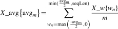 |
where X ∈ {PSSM_{AAj}, SS_{SSk}, RSA, IUPREDL, IUPREDS, DISOPRED, DISOCLUST} is the name of a given feature, AAj with j ∈ {1, 2,…, 20} is the amino acid type, SSk with k ∈ {H, E, C} is the type of the SS, avgm with m ∈ {3, 5, 7,…39, 41} is the size of the window, wn with n ∈ {−20, −19,…, 19, 20} is the position in the window where 0 denotes the position of the predicted residue, and X_w{wn} is the value of feature X for the residue at position wn (the actual position in the sequence equals i+wn). When aggregating, we ignore the positions in the window that are outside of the chain for the residues close to the sequence terminus, i.e. we sum only the values for the positions in the chain and this sum is dived by the total number of these positions. The features are divided into 17 categories based on the source information used including sequence, PSSM, amino-acid frequency, conservation, SS, RSA, torsion angles, DISOPRED2, DISOclust, IUPREDL, IUPREDS, B-factor, signal peptides, purification tag, globular domains, strict flexibility and non-strict flexibility. Detailed description is provided in the appendix at http://biomine.ece.ualberta.ca/MFDp.html.
2.6 Feature selection and parameterization of SVMs
We designed three SVMs using different versions of the MxD dataset. The SVMALL was designed using the entire MxD dataset, while SVMLONG and SVMSHORT were developed using the MxD dataset where the disorder residues from short (<30 residues) and from long (≥30 residues) disorder segments were removed, respectively. For each of the three models we used the following procedure. In the ‘first step’ we remove all highly correlated features within each of the 17 feature categories. For each feature we compute its average biserial correlation (over five correlations computed from the five training subsets of the MxD dataset) with the outcomes, i.e. annotation of ordered and disorder residues. We sort the features in each category according to their average biserial correlations. The set of the selected features is initialized with the feature that has the highest biserial correlation. Next, for each following features we calculate its average correlation (over the five training subsets) with any of the features which were already selected, and we add it to the set of selected features only if the correlation <0.9. We discard the features that were not selected. In the ‘second step’ we quantify predictive quality of the features selected in the first step using the linear SVMs. We construct feature sets by selecting top t features, according to their average biserial correlations, from each category. We take all features in a given category if their number <t. Next, we run 5-fold cross validation on the MxD dataset where we vary the value of t between 1 and 15, and for each t we parameterize the value of constant C of the linear SVM classifiers. We consider C in consecutive powers of 2 between 2−8 and 25. For each of the prediction models (ALL, LONG and SHORT) t = 1 provides the best values of AUC in the 5-fold cross validation on the MxD dataset. Next, starting from the least correlated feature from the selected 17 features, we removed a given feature if it increases AUC value for the 5-fold cross validation-based prediction on the MxD dataset; this lead to removal of the features related to the annotation of the signal peptides. For the remaining relevant feature categories, we attempt to add additional features which improve predictive quality. For each of the remaining categories, starting with the category with the most correlated feature, we keep adding features (starting with second-best feature from the category) as long as the addition of a feature increased the AUC value for the 5-fold cross validation on the MxD dataset. For each removal/addition, we tuned the C parameter of the SVM. For the ALL model, we selected 16 features from 11 categories; for the SHORT model, we selected 30 features from 12 categories; and for the LONG model, we have 17 features from 12 categories. The selected features are shown in the Table 1 in the appendix at http://biomine.ece.ualberta.ca/MFDp.html. A significant fraction of the features (27 out of the entire set of 63) are based on the aggregated information, which suggests that our features provide better discriminatory power than the raw values. The selected features consider almost all sources, except for the signal peptides annotations.
The entire process, including feature selection and SVM parameterization, was consistently carried using 5-fold cross validation on MxD dataset.
3 RESULTS
3.1 Comparison with existing predictors
We compare MFDp with relevant predictors on the MxD and CASP8 datasets. For the MxD dataset, we use 5-fold cross validation to assess our predictions; we use 75% of each of the five training subsets to compute SVMs, the other 25% to find the threshold used for binarization of the probabilities, and the test subsets to evaluate predictions. In contrast, predictions from other method are generated on the entire dataset (without cross-validation) using either web-servers or stand-alone implementations provided by the authors. For the test on the CASP8 dataset, the MFDp is trained, including computation of SVMs (using the same parameters as for the MxD dataset) and the selection of the threshold, using all fully disordered and PDB chains in the MxD dataset; these chains have similar disorder characteristics to the chains in the CASP8. The training chains from the MxD dataset share at most 25% identity to any chain the CASP8 set making it challenging to perform predictions. On the contrary, the methods we compare with use large training datasets that may share substantial similarity to the CASP8 targets (i.e only a handful of CASP8 target were consider as free-modeling), which could raise their predictive quality.
The cross-validated predictions of MFDp are compared to its input predictors, including: DISOPRED2; IUPredL and IUPredS (IUPred predictions for short and long segments); DISOclust; and PROFBval, and with selected other recent methods including the consensus-based MD (Schlessinger et al., 2009), the propensity-based Ucon (Schlessinger et al., 2007a) and the machine learning-based NORSnet (Schlessinger et al., 2007b). Our results on the CASP8 dataset are also compared against five top-performing methods in the CASP8 experiments (Noivirt-Brik et al., 2009). These methods are identified by the group number in square brackets (as registered for the CASP8 meeting) and the group name. They include GS-MetaServer2 [153], GeneSilicoMetaServer [297], MULTICOM-CMFR [69] (Cheng et al., 2005), DISOclust [97] (McGuffin, 2008) and McGuffin [379], which is a human-based consensus that uses DISOclust. More detailed description of these predictors can be found in the CASP8 abstracts at http://predictioncenter.org/casp8/doc/CASP8_book.pdf.
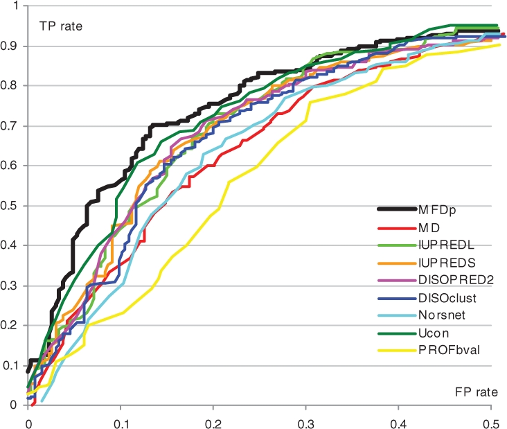
We compare predictive quality when considering all disordered regions and for the regions that are at least 30 residues long, respectively. The selection of the length threshold is consistent with values used in the recent investigation of protein–protein recognition mechanisms (Tompa et al. 2009) and in design of predictors for long segments (Han et al. 2009; Peng et al. 2006). The same as in the CASP8, we discard the disordered regions with three or fewer residues (Noivirt-Brik et al., 2009; private correspondence with authors), i.e. these residues are ignored when computing the quality measures. Similarly, for the results on the long segments we discard the shorter regions. Following the CASP8, predictions were assessed using bootstrapping in which 80% of the targets were randomly selected 1000 times and we report the corresponding averages and standard deviations see Tables 2 and 3. We recomputed the results for the CASP8 submissions and we found them consistent with the original report (Noivirt-Brik et al., 2009). We also analyze statistical significance of the differences between MFDp and the other methods. We compared the 1000 paired average results for MCC, Sw and AUC obtained from using the bootstrapping with 80% of the targets on both CASP8 and MxD datasets. Since the averages do not follow normal distribution, as tested using Shapiro–Wilk test at the 0.05 significance, we use Wilcoxon rank sum test and we measure significance of the differences at 0.01 level. Tables 2 and 3 show that MFDp consistently outperforms all methods based on the MCC index. These improvements are statistically significant with P < 0.01 when compared with all considered competitors on both datasets and for both all and long-disordered segments, except for NORSnet and IUPREDL on the long regions and the CASP8 dataset. Results on the MxD dataset demonstrate that MFDp significantly outperforms its input methods as well as MD, NORSnet and Ucon when considering the Sw and AUC values and for both all and long-disordered segments. Only MD method is shown to be comparable with respect to the AUC values. For the prediction of both all and long segments on the smaller CASP8 dataset, the MFDp significantly improves over its input predictors, MD, NORSnet and Ucon for the binary prediction measured using MCC and Sw. The fact that MFDp is successful in maintaining high-quality predictions for the long segments is important given that predictors designed for long disordered regions are usually less successful in predicting short regions (Obradovic et al., 2005; Peng et al., 2005). Our method is outperformed on the Sw and AUC values for the prediction of all segments by the top five CASP8 methods, but we significantly improve over these methods based on the MCC index. We also significantly improve over their binary assignments, measured with MCC and Sw, for the long-disordered segments. Our improvement are achieved in spite of the fact that our training chains share <25% identity to CASP8 targets, while the top predictors in CASP8 use training sequences that likely share more significant similarity. Moreover, the GS-MetaServer2 [153] and GeneSilicoMetaServer [297] are unpublished and do not offer implementations/servers. The McGuffin [379] method is not automated and requires human expert and the DISOclust [97] results submitted to CASP8 are better than the results generated by the stand-alone DISOclust provided to us by the authors. The MFDp is available as an automated web server at http://biomine.ece.ualberta.ca/MFDp.html. The ROCs for the predictions on both datasets are shown in Figure 2. This figure focuses on the FP rates < 0.5; the entire curve is given in the appendix at http://biomine.ece.ualberta.ca/MFDp.html. The curve reveals that MFDp provides favorable TP rates for the FP values between 0 and 0.4 on the MxD dataset and between 0.1 and 0.4 on the CASP8 dataset when compared with all predictors except the top-performing methods in the CASP8. Our method provides comparable TP rates for the FP rates >0.2 when compared with the top performers from the CASP8 experiment. Overall, we conclude that MFDp outperforms modern existing predictors for binary disorder predictions and provides competitive real-valued predictions.
Table 2.
Comparison of predictive quality measured on the MxD and CASP8 datasets when considering all disordered regions
| Dataset | Predictor | MCC |
Sw |
ACC |
SENS |
SPEC |
AUC |
|||||||||
|---|---|---|---|---|---|---|---|---|---|---|---|---|---|---|---|---|
| Value | SD | Signif- | Value | SD | Signif- | Value | SD | Value | SD | Value | SD | Value | SD | Signif- | ||
| icance | icance | icance | ||||||||||||||
| MxD | MFDp | 0.44 | ±0.02 | 0.51 | ±0.01 | 0.75 | ±0.01 | 0.76 | ±0.01 | 0.75 | ±0.01 | 0.81 | ±0.01 | |||
| MD | 0.43 | ±0.02 | + | 0.48 | ±0.01 | + | 0.74 | ±0.01 | 0.68 | ±0.01 | 0.80 | ±0.01 | 0.81 | ±0.01 | = | |
| DISOPRED2 | 0.40 | ±0.02 | + | 0.44 | ±0.02 | + | 0.72 | ±0.01 | 0.66 | ±0.01 | 0.78 | ±0.01 | 0.78 | ±0.01 | + | |
| IUPredL | 0.39 | ±0.02 | + | 0.42 | ±0.01 | + | 0.71 | ±0.01 | 0.60 | ±0.01 | 0.82 | ±0.01 | 0.78 | ±0.01 | + | |
| IUPredS | 0.37 | ±0.01 | + | 0.38 | ±0.01 | + | 0.69 | ±0.01 | 0.53 | ±0.01 | 0.85 | ±0.01 | 0.78 | ±0.01 | + | |
| NORSnet | 0.34 | ±0.02 | + | 0.37 | ±0.02 | + | 0.68 | ±0.01 | 0.55 | ±0.02 | 0.81 | ±0.01 | 0.74 | ±0.01 | + | |
| DISOclust | 0.33 | ±0.01 | + | 0.40 | ±0.01 | + | 0.70 | ±0.01 | 0.78 | ±0.01 | 0.62 | ±0.01 | 0.77 | ±0.01 | + | |
| Ucon | 0.31 | ±0.01 | + | 0.34 | ±0.01 | + | 0.67 | ±0.01 | 0.57 | ±0.01 | 0.77 | ±0.01 | 0.74 | ±0.01 | + | |
| PROFbval | 0.19 | ±0.01 | + | 0.22 | ±0.01 | + | 0.61 | ±0.00 | 0.84 | ±0.01 | 0.38 | ±0.01 | 0.69 | ±0.01 | + | |
| CASP8 | MFDp | 0.61 | ±0.06 | 0.63 | ±0.06 | 0.82 | ±0.03 | 0.68 | ±0.06 | 0.95 | ±0.00 | 0.89 | ±0.02 | |||
| 379 | 0.59 | ±0.06 | + | 0.65 | ±0.05 | – | 0.82 | ±0.03 | 0.71 | ±0.05 | 0.94 | ±0.00 | 0.91 | ±0.02 | – | |
| DISOPRED2 | 0.59 | ±0.06 | + | 0.61 | ±0.06 | + | 0.80 | ±0.03 | 0.65 | ±0.06 | 0.95 | ±0.00 | 0.88 | ±0.02 | + | |
| 297 | 0.57 | ±0.05 | + | 0.66 | ±0.05 | – | 0.83 | ±0.02 | 0.74 | ±0.05 | 0.92 | ±0.00 | 0.90 | ±0.02 | – | |
| 97 | 0.56 | ±0.05 | + | 0.65 | ±0.05 | – | 0.82 | ±0.02 | 0.73 | ±0.05 | 0.92 | ±0.00 | 0.91 | ±0.02 | – | |
| 153 | 0.55 | ±0.05 | + | 0.67 | ±0.05 | – | 0.83 | ±0.02 | 0.76 | ±0.05 | 0.90 | ±0.00 | 0.91 | ±0.02 | – | |
| IUPredS | 0.54 | ±0.06 | + | 0.52 | ±0.06 | + | 0.76 | ±0.03 | 0.56 | ±0.06 | 0.96 | ±0.00 | 0.85 | ±0.03 | + | |
| IUPredL | 0.53 | ±0.09 | + | 0.45 | ±0.09 | + | 0.73 | ±0.05 | 0.48 | ±0.09 | 0.98 | ±0.00 | 0.82 | ±0.03 | + | |
| 69 | 0.51 | ±0.05 | + | 0.66 | ±0.04 | – | 0.83 | ±0.02 | 0.80 | ±0.04 | 0.86 | ±0.00 | 0.90 | ±0.02 | – | |
| NORSnet | 0.48 | ±0.12 | + | 0.37 | ±0.11 | + | 0.69 | ±0.06 | 0.39 | ±0.11 | 0.98 | ±0.00 | 0.79 | ±0.04 | + | |
| DISOclust | 0.42 | ±0.05 | + | 0.59 | ±0.04 | + | 0.80 | ±0.02 | 0.78 | ±0.04 | 0.82 | ±0.01 | 0.86 | ±0.02 | + | |
| MD | 0.42 | ±0.06 | + | 0.56 | ±0.06 | + | 0.78 | ±0.03 | 0.71 | ±0.06 | 0.85 | ±0.01 | 0.85 | ±0.03 | + | |
| Ucon | 0.29 | ±0.06 | + | 0.34 | ±0.07 | + | 0.67 | ±0.03 | 0.47 | ±0.07 | 0.87 | ±0.00 | 0.74 | ±0.04 | + | |
| PROFbval | 0.19 | ±0.03 | + | 0.31 | ±0.03 | + | 0.65 | ±0.01 | 0.86 | ±0.03 | 0.45 | ±0.01 | 0.78 | ±0.03 | + | |
We report the averages and corresponding SDs for bootstrapping with 1000 repetitions of 80% of chains. Underlined methods are used as inputs for MFDp. The methods are sorted by the MCC values and the highest values are shown in bold. Results of tests of significance of the differences between MFDp and the other methods are given in the ‘significance’ columns. The tests compare average values from 1000 bootstrapping repetitions. The + and – mean that MFDp is statistically significantly better/worse with P < 0.01, and = means that results are not significantly different.
Table 3.
Comparison of predictive quality measured on the MxD and CASP8 datasets when considering disordered regions that are ≥30-residues long
| Dataset | Predictor | MCC |
Sw |
ACC |
SENS |
SPEC |
AUC |
|||||||||
|---|---|---|---|---|---|---|---|---|---|---|---|---|---|---|---|---|
| Value | SD | Signif- | Value | SD | Signif- | Value | SD | Value | SD | Value | SD | Value | SD | Signif- | ||
| icance | icance | icance | ||||||||||||||
| MxD | MFDp | 0.44 | ±0.02 | 0.52 | ±0.02 | 0.76 | ±0.01 | 0.77 | ±0.01 | 0.75 | ±0.01 | 0.82 | ±0.01 | |||
| MD | 0.44 | ±0.02 | + | 0.50 | ±0.02 | + | 0.75 | ±0.01 | 0.70 | ±0.01 | 0.80 | ±0.01 | 0.82 | ±0.01 | = | |
| IUPredL | 0.41 | ±0.02 | + | 0.45 | ±0.01 | + | 0.72 | ±0.01 | 0.63 | ±0.01 | 0.82 | ±0.01 | 0.79 | ±0.01 | + | |
| DISOPRED2 | 0.40 | ±0.02 | + | 0.46 | ±0.02 | + | 0.73 | ±0.01 | 0.67 | ±0.02 | 0.78 | ±0.01 | 0.78 | ±0.01 | + | |
| NORSnet | 0.37 | ±0.02 | + | 0.41 | ±0.02 | + | 0.70 | ±0.01 | 0.59 | ±0.02 | 0.81 | ±0.01 | 0.76 | ±0.01 | + | |
| IUPredS | 0.37 | ±0.01 | + | 0.38 | ±0.01 | + | 0.69 | ±0.01 | 0.53 | ±0.01 | 0.85 | ±0.01 | 0.78 | ±0.01 | + | |
| DISOclust | 0.33 | ±0.01 | + | 0.40 | ±0.01 | + | 0.70 | ±0.01 | 0.79 | ±0.01 | 0.62 | ±0.01 | 0.77 | ±0.01 | + | |
| Ucon | 0.32 | ±0.01 | + | 0.37 | ±0.01 | + | 0.68 | ±0.01 | 0.60 | ±0.01 | 0.77 | ±0.01 | 0.75 | ±0.01 | + | |
| PROFbval | 0.19 | ±0.01 | + | 0.22 | ±0.01 | + | 0.61 | ±0.00 | 0.84 | ±0.01 | 0.38 | ±0.01 | 0.70 | ±0.01 | + | |
| CASP8 | MFDp | 0.60 | ±0.10 | 0.73 | ±0.09 | 0.86 | ±0.04 | 0.78 | ±0.09 | 0.95 | ±0.00 | 0.90 | ±0.04 | |||
| NORSnet | 0.59 | ±0.16 | = | 0.57 | ±0.16 | + | 0.79 | ±0.08 | 0.59 | ±0.17 | 0.98 | ±0.00 | 0.87 | ±0.05 | + | |
| IUPredL | 0.59 | ±0.15 | = | 0.60 | ±0.15 | + | 0.80 | ±0.07 | 0.62 | ±0.15 | 0.98 | ±0.00 | 0.85 | ±0.06 | + | |
| DISOPRED2 | 0.58 | ±0.11 | + | 0.68 | ±0.10 | + | 0.84 | ±0.05 | 0.73 | ±0.10 | 0.95 | ±0.00 | 0.90 | ±0.04 | = | |
| 379 | 0.56 | ±0.10 | + | 0.71 | ±0.08 | + | 0.86 | ±0.04 | 0.77 | ±0.08 | 0.94 | ±0.00 | 0.93 | ±0.03 | – | |
| 297 | 0.54 | ±0.09 | + | 0.73 | ±0.08 | + | 0.87 | ±0.04 | 0.81 | ±0.08 | 0.92 | ±0.00 | 0.91 | ±0.04 | – | |
| IUPredS | 0.53 | ±0.11 | + | 0.59 | ±0.10 | + | 0.79 | ±0.05 | 0.63 | ±0.10 | 0.96 | ±0.00 | 0.86 | ±0.05 | + | |
| 97 | 0.52 | ±0.09 | + | 0.71 | ±0.08 | + | 0.85 | ±0.04 | 0.79 | ±0.08 | 0.92 | ±0.00 | 0.93 | ±0.03 | – | |
| 153 | 0.50 | ±0.09 | + | 0.72 | ±0.08 | + | 0.86 | ±0.04 | 0.81 | ±0.08 | 0.90 | ±0.00 | 0.92 | ±0.03 | – | |
| 69 | 0.44 | ±0.08 | + | 0.69 | ±0.07 | + | 0.85 | ±0.03 | 0.83 | ±0.07 | 0.86 | ±0.00 | 0.91 | ±0.03 | – | |
| DISOclust | 0.37 | ±0.07 | + | 0.63 | ±0.07 | + | 0.81 | ±0.04 | 0.81 | ±0.07 | 0.82 | ±0.01 | 0.88 | ±0.04 | + | |
| MD | 0.36 | ±0.09 | + | 0.58 | ±0.11 | + | 0.79 | ±0.05 | 0.73 | ±0.11 | 0.85 | ±0.01 | 0.86 | ±0.05 | + | |
| Ucon | 0.28 | ±0.09 | + | 0.41 | ±0.12 | + | 0.71 | ±0.06 | 0.54 | ±0.12 | 0.87 | ±0.00 | 0.77 | ±0.06 | + | |
| PROFbval | 0.16 | ±0.04 | + | 0.31 | ±0.05 | + | 0.66 | ±0.03 | 0.87 | ±0.05 | 0.45 | ±0.01 | 0.81 | ±0.06 | + | |
We report the averages and corresponding SDs for bootstrapping with 1000 repetitions of 80% of chains. Underlined methods are used as inputs for MFDp. The methods are sorted by the MCC values and the highest values are shown in bold. Results of tests of significance of the differences between MFDp and the other methods are given in the ‘significance’ columns. The tests compare average values from 1000 bootstrapping repetitions. The + and − mean that MFDp is statistically significantly better/worse with P < 0.01, and = means that results are not significantly different.
Fig. 2.

ROCs for the predictions on the (A) MxD and (B) CASP8 datasets.
3.2 Predictions of proteins with long-disordered segments
We investigate the quality of our predictions applied to find proteins with long (≥ 30 residues)-disordered regions. This binary prediction is motivated by the fact that this information is useful for target selection (Punta et al., 2009; Slabinski et al., 2007) and protein–protein recognition (Tompa et al., 2009). Similar evaluation was also performed for the MD (Schlessinger et al., 2009). Although ∼43% of disordered residues in CASP8 are in the long segments (allowing for a relatively robust per-residues evaluations), there are only 15 such segments and thus we did not use this dataset. The results on the MD dataset obtained using 5-fold cross validation for the MFDp and the predictions from the servers for MD, DISOPRED2, IUPred, NORSnet, DISOclust, Ucon and PROFbval are summarized in Table 4. The corresponding ROC curves are shown in Figure 3 (for 0–0.5-TP-rate range) and in the appendix (for the entire range). The results demonstrate that MFDp outperforms all considered predictors as measured using MCC, ACC and AUC values. This suggests that our method is a useful resource for annotation of proteins with long disordered regions.
Table 4.
Comparison of predictions of proteins with long (≥ 30 residues) disordered segments on the MxD datasets
| Predictor | MCC | ACC | SENS | SPEC | AUC |
|---|---|---|---|---|---|
| MFDp | 0.53 | 0.77 | 0.82 | 0.71 | 0.86 |
| Ucon | 0.52 | 0.73 | 0.53 | 0.95 | 0.85 |
| DISOPRED2 | 0.52 | 0.76 | 0.71 | 0.81 | 0.82 |
| IUPredS | 0.52 | 0.75 | 0.63 | 0.87 | 0.83 |
| IUPredL | 0.51 | 0.74 | 0.60 | 0.89 | 0.83 |
| MD | 0.49 | 0.74 | 0.67 | 0.81 | 0.80 |
| NORSnet | 0.48 | 0.71 | 0.51 | 0.93 | 0.80 |
| DISOclust | 0.47 | 0.73 | 0.84 | 0.62 | 0.82 |
| PROFbval | 0.39 | 0.69 | 0.73 | 0.66 | 0.76 |
Underlined methods are used as inputs for MFDp. The methods are sorted by the MCC values and the highest values are shown in bold.
Fig. 3.
ROCs for the predictions of proteins with long-disordered segments on the MxD dataset.
3.3 Case studies
We selected CASP8 target T0480 (PDBid 2K4X) which was solved with NMR, and CASP8 target T0404 (PDBid 2DFE) which was solved with X-ray crystallography, as our case studies. We compare side-by-side prediction of MFDp, its input predictors DISOPRED2, IUPred, DISOclust, the recent ensemble-based MD, and two top-performing on the CASP8 (with respect to MCC) McGuffin [379] and GeneSilicoMetaServer [297] methods (Fig. 4). For the T0480, which is a small protein with ∼50% disordered residues located at sequence termini, MFDp finds both disordered segments, achieves below-average MCC of 0.59 and improves over predictions of its ensemble predictors. The MD over-predicts disorder and GeneSilicoMetaServer generates predictions comparable to that of MFDp. The T0404 includes 25% disordered residues with one longer segment away from the termini. Most of the predictors find both disordered segments, and they also incorrectly annotate another disordered segment at the N-terminus, except IUPREDL which predicts only the middle segment. The GeneSilicoMetaServer and MD slightly over-predict disorder, and the segment in the center of the chain is most accurately predicted by MFDp, DISOPRED2 and McGuffin. Although these predictions should not be assumed typical, they demonstrate that the MFDp can outperform all of its input predictors.
Fig. 4.

Comparison of predictions from MFDp, DISOPRED2 (DP2), IUPREDL (IUPL), IUPREDS (IUPS) and DISOclust (DISOc), MD; and two CASP8 predictors with the highest MCC, McGuffin (379) and GeneSilicoMetaServer (297) for CASP8 targets T0480 (on the left) and T0404 (on the right). The ‘–’ and ‘D’ denote the ordered and disordered residues, respectively. The actual disorder annotations are shown in the first line.
4 CONCLUSIONS
The MFDp predicts disordered regions of all sizes and different types. On average, it improves over the predictions of current solutions for the binary disorder assignment and provides competitive real-value predictions, as evaluated on two datasets with low-sequence similarity. The MFDp's outputs are also shown to outperform other predictors for the identification of proteins with long-disordered regions. The main reasons for the improvements are the application of a comprehensive set of information sources including complementary disorder predictions, sequence profiles and other relevant sequence-based predictors of structural and functional protein characteristics, novel two-layer architecture and the usage of custom features that aggregate raw prediction inputs.
Funding: NSERC Canada (to L.K.); Icore/Alberta Ingenuity Scholarships (to W.S., K.C. and K.D.K.).
Conflict of Interest: none declared.
Supplementary Material
REFERENCES
- Altschul SF, et al. Gapped BLAST and PSI-BLAST: a new generation of protein database search programs. Nucleic Acids Res. 1997;25:3389–3402. doi: 10.1093/nar/25.17.3389. [DOI] [PMC free article] [PubMed] [Google Scholar]
- Berman HM, et al. The Protein Data Bank. Nucleic Acids Res. 2000;28:235–242. doi: 10.1093/nar/28.1.235. [DOI] [PMC free article] [PubMed] [Google Scholar]
- Bordoli L, et al. Assessment of disorder predictions in CASP7. Proteins. 2007;69(Suppl. 8):129–136. doi: 10.1002/prot.21671. [DOI] [PubMed] [Google Scholar]
- Cheng J, et al. Accurate prediction of protein disordered regions by mining protein structure data. Data Mining Knowl. Disc. 2005;11:213–222. [Google Scholar]
- Dosztányi Z, et al. IUPred: web server for the prediction of intrinsically unstructured regions of proteins based on estimated energy content. Bioinformatics. 2005;21:3433–3434. doi: 10.1093/bioinformatics/bti541. [DOI] [PubMed] [Google Scholar]
- Dunker AK, et al. The unfoldomics decade: an update on intrinsically disordered proteins. BMC Genomics. 2008;9(Suppl. 2):S1. doi: 10.1186/1471-2164-9-S2-S1. [DOI] [PMC free article] [PubMed] [Google Scholar]
- Dyson HJ, Wright PE. Intrinsically unstructured proteins and their functions. Nat. Rev. Mol. Cell. Biol. 2005;6:197–208. doi: 10.1038/nrm1589. [DOI] [PubMed] [Google Scholar]
- Fan R-E, et al. LIBLINEAR: a library for large linear classification. J. Mach. Learn. Res. 2008;9:1871–1874. [Google Scholar]
- Faraggi E, et al. Improving the prediction accuracy of residue solvent accessibility and real-value backbone torsion angles of proteins by fast guided-learning through a two-layer neural network. Proteins. 2009;74:857–871. doi: 10.1002/prot.22193. [DOI] [PMC free article] [PubMed] [Google Scholar]
- Han P, et al. Large-scale prediction of long disordered regions in proteins using random forests. BMC Bioinformatics. 2009;10:8. doi: 10.1186/1471-2105-10-8. [DOI] [PMC free article] [PubMed] [Google Scholar]
- Hecker J, et al. Protein disorder prediction at multiple levels of sensitivity and specificity. BMC Genomics. 2008;9(Suppl. 1):S9. doi: 10.1186/1471-2164-9-S1-S9. [DOI] [PMC free article] [PubMed] [Google Scholar]
- Hirose S, et al. POODLE-L: a two-level SVM prediction system for reliably predicting long disordered regions. Bioinformatics. 2007;23:2046–2053. doi: 10.1093/bioinformatics/btm302. [DOI] [PubMed] [Google Scholar]
- Ishida T, Kinoshita K. PrDOS: prediction of disordered protein regions from amino acid sequence. Nucleic Acids Res. 2007;35:W460–W464. doi: 10.1093/nar/gkm363. [DOI] [PMC free article] [PubMed] [Google Scholar]
- Ishida T, Kinoshita K. Prediction of disordered regions in proteins based on the meta approach. Bioinformatics. 2008;24:1344–1348. doi: 10.1093/bioinformatics/btn195. [DOI] [PubMed] [Google Scholar]
- Jones DT, Swindells MB. Getting the most from PSI-BLAST. Trends Biochem. Sci. 2002;27:161–164. doi: 10.1016/s0968-0004(01)02039-4. [DOI] [PubMed] [Google Scholar]
- Jones DT, Ward JJ. Prediction of disordered regions in proteins from position specific score matrices. Proteins. 2003;53(Suppl. 6):573–578. doi: 10.1002/prot.10528. [DOI] [PubMed] [Google Scholar]
- Linding R, et al. GlobPlot: exploring protein sequences for globularity and disorder. Nucleic Acids Res. 2003;31:3701–3708. doi: 10.1093/nar/gkg519. [DOI] [PMC free article] [PubMed] [Google Scholar]
- McGuffin LJ. Intrinsic disorder prediction from the analysis of multiple protein fold recognition models. Bioinformatics. 2008;24:1798–1804. doi: 10.1093/bioinformatics/btn326. [DOI] [PubMed] [Google Scholar]
- McGuffin LJ, et al. The PSIPRED protein structure prediction server. Bioinformatics. 2000;16:404–405. doi: 10.1093/bioinformatics/16.4.404. [DOI] [PubMed] [Google Scholar]
- Noivirt-Brik O, et al. Assessment of disorder predictions in CASP8. Proteins. 2009;77(Suppl. 9):210–216. doi: 10.1002/prot.22586. [DOI] [PubMed] [Google Scholar]
- Obradovic Z, et al. Exploiting heterogeneous sequence properties improves prediction of protein disorder. Proteins. 2005;61:176–182. doi: 10.1002/prot.20735. [DOI] [PubMed] [Google Scholar]
- Oldfield CJ, et al. Comparing and combining predictors of mostly disordered proteins. Biochemistry. 2005;44:1989–2000. doi: 10.1021/bi047993o. [DOI] [PubMed] [Google Scholar]
- Peng K, et al. Optimizing intrinsic disorder predictors with protein evolutionary information. J. Bioinform. Comput. Biol. 2005;3:35–60. doi: 10.1142/s0219720005000886. [DOI] [PubMed] [Google Scholar]
- Peng K, et al. Length-dependent prediction of protein intrinsic disorder. BMC Bioinformatics. 2006;7:208. doi: 10.1186/1471-2105-7-208. [DOI] [PMC free article] [PubMed] [Google Scholar]
- Plewczynski D, et al. Prediction of signal peptides in protein sequences by neural networks. Acta Biochim. Pol. 2008;55:261–267. [PubMed] [Google Scholar]
- Prilusky J, et al. FoldIndex: a simple tool to predict whether a given protein sequence is intrinsically unfolded. Bioinformatics. 2005;21:3435–3438. doi: 10.1093/bioinformatics/bti537. [DOI] [PubMed] [Google Scholar]
- Punta M, et al. Structural genomics target selection for the New York consortium on membrane protein structure. J. Struct. Funct. Genomics. 2009;10:255–268. doi: 10.1007/s10969-009-9071-1. [DOI] [PMC free article] [PubMed] [Google Scholar]
- Radivojac P, et al. Protein flexibility and intrinsic disorder. Prot. Sci. 2004;13:71–80. doi: 10.1110/ps.03128904. [DOI] [PMC free article] [PubMed] [Google Scholar]
- Radivojac P, et al. Intrinsic disorder and functional proteomics. Biophys. J. 2007;92:1439–1456. doi: 10.1529/biophysj.106.094045. [DOI] [PMC free article] [PubMed] [Google Scholar]
- Raychaudhuri S, et al. The role of intrinsically unstructured proteins in neurodegenerative diseases. PLoS One. 2009;4:e5566. doi: 10.1371/journal.pone.0005566. [DOI] [PMC free article] [PubMed] [Google Scholar]
- Schlessinger A, et al. PROFbval: predict flexible and rigid residues in proteins. Bioinformatics. 2006;22:891–893. doi: 10.1093/bioinformatics/btl032. [DOI] [PubMed] [Google Scholar]
- Schlessinger A, et al. Natively unstructured regions in proteins identified from contact predictions. Bioinformatics. 2007a;23:2376–2384. doi: 10.1093/bioinformatics/btm349. [DOI] [PubMed] [Google Scholar]
- Schlessinger A, et al. Natively unstructured loops differ from other loops. PLoS Comput. Biol. 2007b;3:e140. doi: 10.1371/journal.pcbi.0030140. [DOI] [PMC free article] [PubMed] [Google Scholar]
- Schlessinger A, et al. Improved disorder prediction by combination of orthogonal approaches. PLoS One. 2009;4:e4433. doi: 10.1371/journal.pone.0004433. [DOI] [PMC free article] [PubMed] [Google Scholar]
- Shimizu K, et al. POODLE-S: web application for predicting protein disorder by using physicochemical features and reduced amino acid set of a position-specific scoring matrix. Bioinformatics. 2007a;23:2337–2338. doi: 10.1093/bioinformatics/btm330. [DOI] [PubMed] [Google Scholar]
- Shimizu K, et al. Predicting mostly disordered proteins by using structure-unknown protein data. BMC Bioinformatics. 2007b;8:78. doi: 10.1186/1471-2105-8-78. [DOI] [PMC free article] [PubMed] [Google Scholar]
- Sickmeier M, et al. DisProt: the Database of Disordered Proteins. Nucleic Acids Res. 2007;35:D786–D793. doi: 10.1093/nar/gkl893. [DOI] [PMC free article] [PubMed] [Google Scholar]
- Slabinski L, et al. The challenge of protein structure determination - lessons from structural genomics. Prot. Sci. 2007;16:2472–2482. doi: 10.1110/ps.073037907. [DOI] [PMC free article] [PubMed] [Google Scholar]
- Su CT, et al. iPDA: integrated protein disorder analyzer. Nucleic Acids Res. 2007;35:465–472. doi: 10.1093/nar/gkm353. [DOI] [PMC free article] [PubMed] [Google Scholar]
- Su CT, et al. Protein disorder prediction by condensed PSSM considering propensity for order or disorder. BMC Bioinformatics. 2006;7:319. doi: 10.1186/1471-2105-7-319. [DOI] [PMC free article] [PubMed] [Google Scholar]
- Tompa P, et al. Close encounters of the third kind: disordered domains and the interactions of proteins. Bioessays. 2009;31:328–335. doi: 10.1002/bies.200800151. [DOI] [PubMed] [Google Scholar]
- Uversky VN, et al. Why are “natively unfolded” proteins unstructured under physiologic conditions? Proteins. 2000;41:415–427. doi: 10.1002/1097-0134(20001115)41:3<415::aid-prot130>3.0.co;2-7. [DOI] [PubMed] [Google Scholar]
- Vucetic S, et al. Flavors of protein disorder. Proteins. 2003;52:573–584. doi: 10.1002/prot.10437. [DOI] [PubMed] [Google Scholar]
- Vullo A, et al. Spritz server for the prediction of intrinsically disordered regions in protein sequences using kernel machines. Nucleic Acids Res. 2006;34:W164–W168. doi: 10.1093/nar/gkl166. [DOI] [PMC free article] [PubMed] [Google Scholar]
- Wang G, Dunbrack RL., Jr. PISCES: a protein sequence culling server. Bioinformatics. 2003;19:1589–1591. doi: 10.1093/bioinformatics/btg224. [DOI] [PubMed] [Google Scholar]
- Wang L, Sauer UH. OnD-CRF: predicting order and disorder in proteins using conditional random fields. Bioinformatics. 2008;24:1401–1402. doi: 10.1093/bioinformatics/btn132. [DOI] [PMC free article] [PubMed] [Google Scholar]
- Ward JJ, et al. The DISOPRED server for the prediction of protein disorder. Bioinformatics. 2004;20:2138–2139. doi: 10.1093/bioinformatics/bth195. [DOI] [PubMed] [Google Scholar]
- Wu S, Zhang Y. MUSTER: improving protein sequence profile-profile alignments by using multiple sources of structure information. Proteins. 2008;72:547–556. doi: 10.1002/prot.21945. [DOI] [PMC free article] [PubMed] [Google Scholar]
- Yang MQ, Yang JY. Sixth IEEE Symposium on BioInformatics and BioEngineering. Washington DC, USA: IEEE Computer Society; 2006. IUP: intrinsically unstructured protein predictor – a software tool for analyzing polypeptide sequences; pp. 16–18. [Google Scholar]
- Zhang H, et al. On the relation between residue flexibility and local solvent accessibility in proteins. Proteins. 2009;76:617–636. doi: 10.1002/prot.22375. [DOI] [PubMed] [Google Scholar]
Associated Data
This section collects any data citations, data availability statements, or supplementary materials included in this article.