Variance Components in Discrete Force Production Tasks

Abstract

The study addresses the relationships between task parameters and two components of variance, “good” and “bad”, during multi-finger accurate force production. The variance components are defined in the space of commands to the fingers (finger modes) and refer to variance that does (“bad”) and does not (“good”) affect total force. Based on an earlier study of cyclic force production, we hypothesized that speeding-up an accurate force production task would be accompanied by a drop in the regression coefficient linking the “bad” variance and force rate such that variance of the total force remains largely unaffected. We also explored changes in parameters of anticipatory synergy adjustments with speeding-up the task. The subjects produced accurate ramps of total force over different times and in different directions (force-up and force-down) while pressing with the four fingers of the right hand on individual force sensors. The two variance components were quantified, and their normalized difference was used as an index of a total force stabilizing synergy. “Good” variance scaled linearly with force magnitude and did not depend on force rate. “Bad” variance scaled linearly with force rate within each task, and the scaling coefficient did not change across tasks with different ramp times. As a result, a drop in force ramp time was associated with an increase in total force variance, unlike the results of the study of cyclic tasks. The synergy index dropped 100-200 ms prior to the first visible signs of force change. The timing and magnitude of these anticipatory synergy adjustments did not depend on the ramp time. Analysis of the data within an earlier model has shown adjustments in the variance of a timing parameter, although these adjustments were not as pronounced as in the earlier study of cyclic force production. Overall, we observed qualitative differences between the discrete and cyclic force production tasks: Speeding-up the cyclic tasks was associated with better adjustments of the timing accuracy, which helps achieve comparable force variance in tasks with different rates of force production. This does not happen in discrete tasks. The lack of scaling of the anticipatory changes in the synergy index with ramp time represent is the first reported feature that distinguishes anticipatory synergy adjustments from anticipatory postural adjustments. We discuss the differences between the cyclic and discrete tasks within a hierarchical control scheme offered by Schöner.

Introduction

A number of recent publications have emphasized differences in the neural control of discrete and cyclic motor tasks based on theoretical analyses, studies of movement kinematics, and brain activation maps (Sternad and Dean 2003; Schaal et al. 2004; Hogan and Sternad 2007; Ronsse et al. 2009). Most of these studies did not address issues of motor coordination in redundant motor systems, in particular issues of the relations between characteristics of motor variance in such systems and task parameters. In non-redundant systems, indices of force variability (for example, the standard deviation) typically scale with force level (Newell and Carlton 1993; Slifkin and Newell 1999; Christou et al. 2002). In redundant systems, however, this dependence may break down due to co-variation among forces produced by individual effectors (Shinohara et al. 2003, 2004). Such a co-variation stabilizes a performance variable produced by a redundant system as a whole, which is a signature mark of a synergy (reviewed in Latash et al. 2002b, 2007). In this study (and in its earlier companion, Friedman et al. 2009), we focus on differences in synergy characteristics during discrete and cyclic isometric multi-digit actions.

We view the system for movement production as a hierarchy with at least two levels, where the higher level produces a low-dimensional output related to salient characteristics of the motor task (Latash 2010; Latash et al. 2010). Neural processing of this signal by the lower level results in a higher-dimensional set of elemental variables whose values may or may not co-vary across repetitive attempts at the task. Synergies are defined as neural organizations at the lower level of the hierarchy that produce co-variation of elements stabilizing (reducing across-trials variability) of a salient output variable.

To study synergies we have been using the framework of the uncontrolled manifold (UCM) hypothesis (Scholz and Schöner 1999). Within this hypothesis, the space of elemental variables is viewed as consisting of two complementary sub-spaces. One of these sub-spaces (the UCM) corresponds to a fixed value of a potentially important performance variable. The other sub-space is orthogonal to the UCM. To quantify motor synergies, variance in the space of elemental variables is quantified within each of the two sub-spaces per degree-of-freedom (V_UCM and V_ORT). If V_UCM > V_ORT, a conclusion is drawn that there is a synergy of elemental variables stabilizing the performance variable for which the two sub-spaces have been defined.

In a recent study (Friedman et al. 2009), we found evidence for an unusual behavior of V_ORT in cyclic tasks: As expected from earlier studies (Latash et al. 2002a; Goodman et al. 2005), this variance component scaled with force rate over the cycle duration and this scaling persisted over tasks performed at different frequencies. However, the scaling coefficient changed across the tasks with the task frequency in such a way, that V_ORT magnitudes were nearly the same across tasks performed at different frequencies. These results were interpreted within an earlier model by Goodman et al. (2005) as pointing at an ability of the controller to adjust variance of a timing parameter τ to achieve about the same performance variability level across different frequencies.

In this study we ask a question whether the ability of the controller to adjust τ variance is unique for cyclic tasks or it can also be observed in discrete tasks. This question was explored at two levels, behavioral and model. At the behavioral level, we analyzed the relations between the time patterns of V_ORT and of force rate (dF/dt) across different task times. We used a linear regression model to link V_ORT to dF/dt (Latash et al. 2002a) and explored the regression coefficient within this model as a dependent variable across different task times. We also explored quantitative features of force stabilizing synergies using the two variance components (V_UCM and V_ORT) and the index of synergy (ΔV) as dependent variables.

At the model level, we compared variance of τ across different task times within the Goodman et al. (2005) model. The model includes two parameters, b and τ, related to the planned force magnitude and planned timing of force production. It has been shown, in particular, that variance in setting τ (timing variance across trials) affects primarily the V_ORT variance component, while variance in setting b is mostly reflected in the V_UCM component. In particular, the dependence of V_ORT on variance of τ results in a nearly linear dependence of V_ORT on derivative of force with respect to time (see also Latash et al. 2002a). We used the coefficient of variation of τ, CV(τ), estimated based on the data, as a dependent variable and explored its changes with task time in both discrete and cyclic tasks.

Based on an earlier study (Latash et al. 2002a) that, however, did not explore a range of force rates, we hypothesized that the discrete tasks will not show the demonstrated feature of the cyclic tasks, namely the ability to adjust the regression coefficient linking V_ORT and dF/dt and CV(τ) such that the magnitude of V_ORT is preserved across different task times.

A secondary aim of the study has been to explore whether preparation to a faster force production is accompanied by earlier/larger anticipatory synergy adjustments (ASAs). The ASAs are changes in a synergy index computed with respect to a particular performance variable (total force in our study) seen 100-200 ms prior to a planned quick change in that variable (Olafsdottir et al. 2005; Shim et al. 2005). The ASAs have been hypothesized to attenuate synergies that would otherwise act against the planned action. Based on this hypothesis and observations by Shim and his collagues (2005), we expected to see earlier and larger ASAs prior to trials with faster force production. We used the time of the earliest change in the synergy index (with respect to the time of action initiation) and the magnitude of its change by the time of action initiation as dependent variables to address this aim.

Methods

Subjects

Eight right hand dominant subjects, five males and three females (mean ±standard deviation: Age: 27±4 years, weight: 69.5±8 kg, height: 1.72±0.1 m, hand width: 7.9±0.4 cm, hand length: 17.8 ± 1.1 cm) volunteered to participate in the study. All the subjects were healthy and had no known history of any neurological or motor disorders. All the subjects gave informed consent according to the policies of the Office for Research Protections at The Pennsylvania State University.

Experimental setup

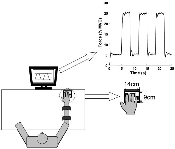
Figure 1 shows the experimental setup. The setup consisted of four one-directional piezoelectric force sensors (model 208C02; PCB Piezotronic Inc.) to measure forces applied in vertical direction by the four finger tips of the right hand. Each of these sensors had a diameter of 1.5 cm and the space between the sensors in the medio-lateral plane was 3 cm. The location of the sensors in the forward-backward direction could be adjusted to match individual subject’s anatomy. The signals from the force sensors were amplified by signal conditioners (M482M66, PCB Piezotronic Inc.) and then sampled at 200 Hz with a 12-bit resolution using a Labview program running on a PC.

Figure 1.

The experimental setup. Subjects pressed on four unidirectional force sensors with the index, middle, ring and little fingers of the right hand. The feedback showed the total force produced by all four fingers. The task was to produce ramp like trajectories between targets shown on the screen. A typical performance is shown for the ramp time of 500 ms.

During the experiment, the subject sat comfortably in a chair facing the test table, with his/her upper arms at approximately 45° of abduction in the frontal plane and approximately 45° of flexion in the sagittal plane. The elbow was flexed at approximately 45°. The forearm was strapped with two pairs of Velcro straps to a wooden board placed on the table so as to prevent movement of the forearm. To ensure that the finger posture does not change during the experiment, we placed a small wooden smooth object under the hand. The subject received task information and feedback on performance through a 17” LCD monitor placed on the table approximately 65 cm from the subject.

Experimental procedure

There were three types of tasks: (1) MVC tasks; (2) Single-finger ramp tasks; and (3) Discrete accurate force production tasks. In all these tasks, subjects received visual feedback on the force produced by the instructed finger(s) via a constantly updating plot of force magnitude (vertical axis) against time (horizontal axis).

In the MVC task, the subjects tried to produce maximal force by each of the four fingers (I - index, M - middle, R - ring, and L - little) and their combination (IMRL). Subjects initially rested all the fingers on the sensors. After the cursor passed a vertical line (at 10 s after the start of the trial), the subjects were required to press “as hard as possible” in a self-paced manner with the instructed finger(s). After reaching a maximum, the subjects were allowed to relax, while still keeping all fingers on the sensors. Each of these trials lasted 30 s. Two trials were recorded for each task finger(s) and the greater force of the two was used in later analysis. The subjects were instructed to keep all four fingers on the sensors, but were told not to pay attention to unintended force production by fingers other than the instructed finger. There was a one-minute rest break between trials. The order of the fingers was randomized across subjects.

In single-finger ramp tasks, the subjects were required to produce force so that the cursor followed a template shown on the screen. This template consisted of a horizontal line at zero force for the first 5 s, then a slanted line from 0% to 40% MVC over the next 10 s and then a horizontal line at 40% MVC for the last 5 s. In each trial, the subject was told to press with one of the fingers to produce force so as to follow the template. The template scale was set such that the top of the screen always corresponded to 50% MVC of the instructed finger. The subjects were required to keep all the fingers on the sensors but were instructed not to pay attention to any unintentional force produced by non-instructed fingers. There was feedback only on the force produced by the instructed finger, not on the forces produced by other fingers. There were two trials for each finger and we block randomized the trials across subjects. There was a 30-s rest between trials. We used the data from these trials to compute the enslaving matrix (see later).

In the accurate force production tasks, the subjects were required to press with the four fingers and produce a force profile that would resemble a ramp. The start and end of the ramps were specified by a cross on the screen. For force increase segments (ramp-up), the starting level was set at 5% MVC of IMRL and the target level was set at 25% MVC of IMRL such that the force amplitude was 20% MVC. For force decrease segments (ramp-down), the starting level was set at 25% MVC IMRL and the target level was set at 5% MVC IMRL. There were five different ramp times: 300 ms, 400 ms, 500 ms, 700 ms and 1400 ms. These times were chosen based on the results of a pilot experiment to cover the range of times within which subjects could successfully perform the task. In all conditions, the subjects were required to hold the final force level for at least 2 s. A sample performance is given in Figure 1. The order of the conditions (ramp times) was block randomized across subjects. For each condition, there were 10 trials with 3 force-up and 3 force-down ramps each. Each trial was 30 s long. In total, the subjects produced 30 force-up ramps and 30 force-down ramps. There were 10-s breaks between trials.

Data processing

The data were processed offline using Matlab (The Mathworks, Natick, MA). The force-up and force-down ramps were analyzed separately. The ramps in each condition were aligned by the point at which the subjects were instructed to start. Force rate (dF/dt) was computed using a five-point derivative after the force data were low-pass filtered with a two-way second-order zero-lag Butterworth filter at 6 Hz.

It is known that, when a subject intends to change force of one finger, other fingers of the hand also show force changes (Kilbreath and Gandevia 1994, Zatsiorsky et al. 2000). To avoid spurious effects of this phenomenon (enslaving) on finger force co-variation indices, we converted the finger force values into finger modes using the corresponding enslaving matrix, E (described below). Finger modes are hypothetical variables that can be manipulated by the central nervous system one at a time. They correspond to intentional involvement of fingers. Changing one mode value leads to proportional force production by all fingers (Zatsiorsky et al. 1998; Danion et al. 2003).

We used single-finger ramp trials to generate the enslaving matrix, E for each subject separately. For each single-finger trial, we performed a linear regression of forces produced by individual fingers against the total force produced by all four fingers over the 10 s ramp. The slopes of the regression lines were used to construct an enslaving matrix, E as follows:

$$\mathrm{E}=\left[\begin{array}{cccc}\hfill {\mathrm{M}}_{\mathrm{I},\mathrm{I}}\hfill & \hfill {\mathrm{M}}_{\mathrm{I},\mathrm{M}}\hfill & \hfill {\mathrm{M}}_{\mathrm{I},\mathrm{R}}\hfill & \hfill {\mathrm{M}}_{\mathrm{I},\mathrm{L}}\hfill \\ \hfill {\mathrm{M}}_{\mathrm{M},\mathrm{I}}\hfill & \hfill {\mathrm{M}}_{\mathrm{M},\mathrm{M}}\hfill & \hfill {\mathrm{M}}_{\mathrm{M},\mathrm{R}}\hfill & \hfill {\mathrm{M}}_{\mathrm{M},\mathrm{L}}\hfill \\ \hfill {\mathrm{M}}_{\mathrm{R},\mathrm{I}}\hfill & \hfill {\mathrm{M}}_{\mathrm{R},\mathrm{M}}\hfill & \hfill {\mathrm{M}}_{\mathrm{R},\mathrm{R}}\hfill & \hfill {\mathrm{M}}_{\mathrm{R},\mathrm{L}}\hfill \\ \hfill {\mathrm{M}}_{\mathrm{L},\mathrm{I}}\hfill & \hfill {\mathrm{M}}_{\mathrm{L},\mathrm{M}}\hfill & \hfill {\mathrm{M}}_{\mathrm{L},\mathrm{R}}\hfill & \hfill {\mathrm{M}}_{\mathrm{L},\mathrm{L}}\hfill \end{array}\right]$$ (1)

where M_i,j are the slopes of the regression line of the force produced by finger i (i = I, M, R, L) with the total force produced by all four fingers when finger j (j = I, M, R, L) was the instructed finger.

The force data from the accurate force production trials, f were converted into mode magnitudes m by using the E matrix: m = [E]⁻¹f

Further, the data from the accurate force production task were analyzed within the framework of the uncontrolled manifold (UCM) hypothesis (Scholz and Schöner 1999). The UCM hypothesis offers a method to decompose variance of elemental variables (m in our study) into two components, one that does not affect the total force (V_UCM) and the other that does (V_ORT). Briefly, for every time sample, the space of elemental variables (m) was divided into two sub-spaces, one that corresponded to a constant value of total force across trials (UCM) and one that led to changes in total force (the space orthogonal to UCM, ORT). Further, we compared variance across trials within each of the subspaces, V_UCM and V_ORT (per dimension). V_UCM > V_ORT was taken as an indication of a multi-digit synergy that stabilized total force.

For each condition and at each point in time, variance components were computed using de-meaned mode data as detailed below: Changes (from the mean) in the modes are given by the vector dm=[dm_i dm_m dm_r dm_l]^T, where T is a sign of transpose. Changes in the value of the total force can be written as a function of dm as follows:

$$d{F}_{TOT}=\left[\begin{array}{cccc}\hfill 1\hfill & \hfill 1\hfill & \hfill 1\hfill & \hfill 1\hfill \end{array}\right]\mathrm{df}=\left[\begin{array}{cccc}\hfill 1\hfill & \hfill 1\hfill & \hfill 1\hfill & \hfill 1\hfill \end{array}\right]\mathrm{E}\mathrm{dm},$$ (2)

where df = [df_i df_m df_r df_l]^T. An orthogonal set of eigenvectors in mode space, e_i defines the sub-space where mode variations do not alter the total force, i.e.

$$0=\left[\begin{array}{cccc}\hfill 1\hfill & \hfill 1\hfill & \hfill 1\hfill & \hfill 1\hfill \end{array}\right]{\mathrm{Ee}}_i$$ (3)

These eigenvectors spanned the null-space of the Jacobian of this transformation ([1 1 1 1] E). Then, the mean-free modes dm were projected onto these directions and summed:

$$f_{\parallel }=\sum _{i=1}^{n-p}\left(e_i^{\mathit{T}}\mathrm{dm}\right)e_i$$ (4)

where n = 4 is the number of degrees of freedom of the m vector, and p=1 is the number of degrees of freedom of the performance variable (F_TOT). The component orthogonal to the null space is given by:

$$f_{\perp }=\mathrm{dm}-f_{\parallel }$$ (5)

The amount of variance per DOF within the UCM is then given by:

$$V_{UCM}=\frac{\sum {\mid f_{\parallel }\mid }^2}{(n-p)N_{trials}}$$ (6)

This is the variance that does not affect the total force. Similarly, the amount of variance per DOF orthogonal to the UCM is given by:

$$V_{ORT}=\frac{\sum _{i=1}^{N_{trials}}{\mid f_{\perp }\mid }^2}{p{N}_{trials}}$$ (7)

This is the variance that affects the total force. Note that V_UCM and V_ORT are normalized per degrees of freedom in the corresponding spaces.

An index of mode co-variation (ΔV) was computed as,

$$\Delta V={\frac{V_{UCM}-V_{ORT}}{V_{TOT}}}_{,}$$ (8)

where V_TOT is the total variance per degree of freedom. Further, ΔV values were z-transformed (adapted to boundaries of ΔV) as:

$$\Delta V_z=0.5\log \left(\frac{4+\Delta V}{1.33-\Delta V}\right)$$ (9)

Relation between variance components and tasks characteristics: Linear model

A linear model to describe the relationship between the two components of variance (V_UCM and V_ORT) and characteristics of the task such as total force magnitude (F_TOT) and its rate of change (dF_TOT/dt) was proposed by Latash et al. (2002). According to this model, for each condition, there is a linear relationship between V_UCM and F_TOT, and a linear relationship between V_ORT and dF_TOT/dt (and, to a lesser extent, F_TOT):

$$V_{UCM}\left(t\right)=a_1\stackrel{‒}{F_{TOT}\left(t\right)}+c_1$$ (10)

$$V_{ORT}\left(t\right)=a_2\stackrel{‒}{F_{TOT}\left(t\right)}+b_2\mid \stackrel{‒}{d{F}_{TOT}\left(t\right)∕dt}\mid +c_2$$ (11)

where $\stackrel{‒}{F_{tot}\left(t\right)}$ and $\mid \stackrel{‒}{dFtot\left(t\right)∕dt}\mid$ are mean total force and mean force rate respectively, a₁ is a coefficient of linear regression that quantifies the dependence of V_UCM on mean total force and c₁ is an error term, a₂ is a coefficient of linear regression that quantifies the dependence of V_ORT on mean total force; b₂ is a coefficient that quantifies the dependence of V_ORT on mean force rate and c₂ is an error term. We slightly modified the model in Latash et al. (2002) to get the model described above (as in an earlier work, Friedman et al. 2009). We used absolute force rate $\mid \stackrel{‒}{dFtot\left(t\right)∕dt}\mid$ rather than force rate dF_TOT(t)/dt to be able to link V_ORT (t) (which is always positive) to dF_TOT(t)/dt (which is negative for force-down ramps). We used this model and fit its parameters, a₁, c₁, a₂, b₂ and c₂ using linear regression, to the observed variances, force, and force rate magnitudes.

Links to Goodman et al. (2005) model of motor variability

Goodman et al. (2005) proposed a model of motor variability within a multi-effector system. According to this model, for multi-finger force production, f(t) profiles of finger forces are defined as:

$$f_{kn}\left(t\right)=b_{kn}{u}_n(t∕{\tau }_{kn}),$$ (12)

where f_kn(t) is the force-time profile produced by a finger n (n = I, M, R, L) in trial k.

This model specifies two scaling parameters b_kn and τ_kn that modify a template u_n(t). These two parameters are chosen randomly from a normal distribution with average values b_n and τ_n and standard deviations SD_bn and SD_τn and are set before each trial. One consequence of this model is that force variance across trials is related to force rate multiplied by a term containing variance of τ, Var(τ), while effects of variance of b are small. Since variance of total force is defined by V_ORT, this model implies that V_ORT is primarily defined by Var(τ).

To analyze how Var(τ) affected V_ORT, we computed the coefficient of variation of the timing parameter τ (CV(τ)) based on the Goodman model and the collected data. Briefly, we related the total force variance with characteristics of task performance (mean force, force rate) as:

$$Var\left(F_{tot}\left(t\right)\right)=\stackrel{‒}{F_{tot}\left(t\right)F_{tot}\left(t\right)}x+t^2\left(\stackrel{‒}{dFtot\left(t\right)∕dt}\right)\left(\stackrel{‒}{dFtot\left(t\right)∕dt}\right)y+\nu \left(t\right),$$ (13)

where Var(F_tot (t)) , $\stackrel{‒}{F_{tot}\left(t\right)}$ , $\stackrel{‒}{dFtot\left(t\right)∕dt}$ are computed for each condition across trials. Using linear regression, we computed the coefficients x and y for each condition for each subject. Note that y in (13) above is related to CV(τ), as follows:

$$CV\left(\tau \right)=\sqrt{y}$$ (14)

Equations (13) and (14) are generalizations of Goodman et al. (2005) model for the four-finger (IMRL) case. Using (14), we computed CV(τ) for each condition for each subject.

Anticipatory synergy adjustments

To study anticipatory synergy adjustments, individual trials were aligned by the time at which the force rate in each particular trial reached 5% of its peak value in that trial (t₀). For this analysis, we considered the data between the following times: 500 ms before t₀ and 100 ms after t₀. The index of mode co-variation across trials (ΔV) was computed and further z-transformed (ΔV_Z) adapted to its boundaries, as explained earlier.

The mean value and standard deviation of ΔV_Z (ΔV_Z-MEAN and ΔV_Z-SD) were computed over the time interval between 500 ms and 300 ms before t₀; this time interval was selected to represent steady-state based on earlier studies (Olafsdottir et al. 2005; Shim et al. 2005). The time of initiation of anticipatory synergy adjustments, t_ASA, was computed for each subject and each condition separately, as the time when ΔV_z dropped below ΔV_Z-MEAN by more than ΔV_Z-SD and stayed below that value until t₀.

To study changes in the magnitude of ΔV_z, we computed an index, ΔΔV_z = ΔV_Z-MEAN - ΔV_Z(t₀), for each subject and each condition.

Statistics

Standard descriptive statistics were used. ANOVA with repeated measures was run on a number of dependent variables.

In order to test whether the variance of total force scaled with ramp time, a two-way repeated measures ANOVA was performed on peak variance of total force with factors Ramp-Time (5 levels) and Direction (2 levels). Direction was included as a factor in order to capture possible differences between the force increase and force decrease trials.

In order to test if V_UCM and V_ORT varied across conditions, we performed a two-way repeated measures ANOVA on peak-to-peak V_UCM and peak V_ORT with factors Ramp-time (5 levels) and Direction (2 levels).

For ΔV analysis, we computed ΔV_z at five equally spaced times (phase 1%, 26%… 100%). To test if ΔV changed across ramp times, or directions, or phases, a repeated measures ANOVA with factors Ramp-time (5 levels), Direction (2 levels) and Phase (5 levels) was used.

To test dependence of V_ORT on absolute magnitude of force rate, we performed a two-way repeated measures ANOVA on the parameter b₂ of the linear model (equation 8) with factors Ramp-time (5 levels) and Direction (2 levels). We used direction as a factor to capture differences between force increase and force decrease ramps.

To test if the CV(τ) varied across ramp times and directions, we performed a two-way repeated measures ANOVA on CV(τ) with factors Ramp-time (5 levels) and Direction (2 levels). To test if ASA magnitude ΔΔV_Z varied across tasks, we performed a two-way repeated measures ANOVA on ΔΔV_Z with factors Ramp-time (5 levels) and Direction (2 levels).

Results

Task performance and patterns of total force variance

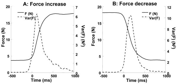
An example of performance in a typical trial is shown in the inset in Figure 1. This figure shows the task with the 500 ms ramp time. Variance of total force was calculated over all trials for force increase and force decrease and for each subject separately. The variance showed a bell shaped profile for all conditions with a peak in the middle of the ramp. Variance at the end of the force increase ramp was slightly higher than that at the beginning of the ramp. Mean performance and variance of performance in one condition by a typical subject in force increase and force decrease trials are shown in Figures 2A and 2B respectively.

Figure 2.

Total force (solid lines) and variance of the total force (dashed lines) averaged across the trials in one condition (ramp time 700 ms) produced by a typical subject. A: force increase, B: force decrease. Note the peak of force variance in the middle of the ramp.

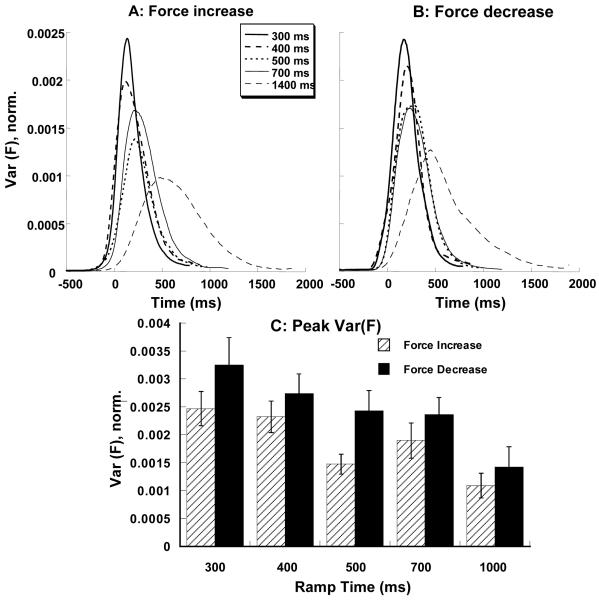
Variance of total force, Var(F), increased as the ramp-time decreased. Figure 3A shows the time profiles of force variance averaged across subjects for the force increase ramps and Figure 3B shows these time profiles for the force decrease ramps. For across-subjects comparisons, all the variances were normalized by the four-finger (IMRL) MVC squared. Figure 3C presents peak values of Var(F) averaged across subjects for both force increase and force decrease ramps. This panel shows that the variance was higher for actions with shorter ramp-times for both force increase and force decrease. It is also clear from Figure 3C that force decrease ramps were characterized by higher Var(F). These observations were confirmed by a two-way repeated measures ANOVA performed on peak variance of total force with factors Ramp-Time (5 levels) and Direction (2 levels). Significant main effects were found for Ramp-Time (F _{(4, 63)} = 13.31, p < 0.001) and Direction (F _{(1, 63)} = 15.5, p < 0.001), without a significant interaction. Pair-wise comparisons showed that the peak Var(F) for the 1400 ms ramp time tasks was significantly different from peak Var(F) in all other tasks, peak Var(F) in the 700 ms tasks was significantly different from that in the 300 ms tasks, and peak Var(F) in the 500 ms tasks was significantly different from that in the 300 ms tasks. The effect of Direction corresponded to higher Var(F) values for the force decrease ramps, compared to the force increase ramps.

Figure 3.

Variance of total force, Var(F), averaged across subjects for different ramp times. Variance values were normalized by MVC squared. A: Var(F) time profiles for the force increase ramps, B: Var(F) time profiles for the force decrease ramps, C: Peak force variance for the different ramp times and two directions of force change. Averaged across subjects data with standard error bars are shown.

Variance within and orthogonal to the uncontrolled manifold

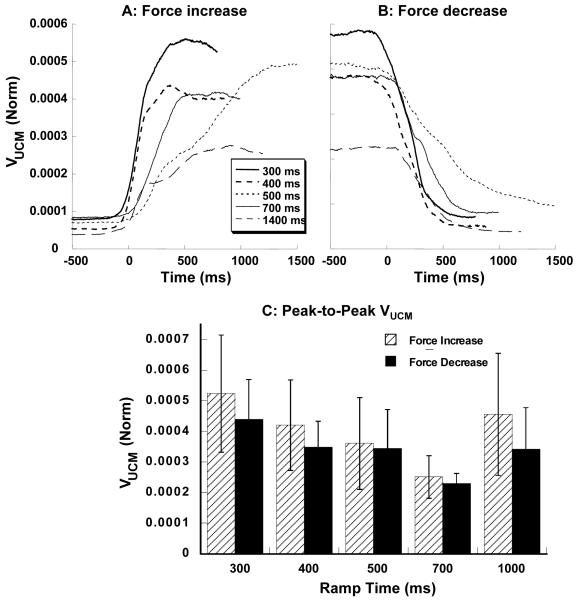
Further, finger force data were transformed into finger modes (see Methods), and the variance in the finger mode space was quantified separately in two sub-spaces: The uncontrolled manifold (UCM) and its orthogonal complements (ORT). Variance within the UCM (V_UCM) and orthogonal to the UCM (V_ORT) were computed using equations 6 and 7, respectively, for each subject and condition. Across subjects and conditions, time profiles of V_UCM resembled the F(t) time profiles. V_UCM increased with force increase and decreased with force decrease. Patterns of V_UCM time profiles for various conditions, averaged across subjects, are presented in Figure 4A for the force increase ramps and in Figure 4B for the force decrease ramps. Note that this index is normalized by MVC squared and number of dimensions (n = 3). Figure 4C shows the normalized peak-to-peak VUCM values for the force increase and force decrease ramps. A two-way repeated measures ANOVA on peak-to-peak V_UCM, with factors Ramp-Time (5 levels) and Direction (2 levels) showed a significant effect of Ramp-Time (F _{(4, 63)} = 2.75, p < 0.05) but not Direction; there was no interaction. Pair-wise contrasts showed that the effect of Ramp-Time corresponded to a significant difference between the 700 ms ramp tasks and the 300 ms ramp tasks.

Figure 4.

Variance within the UCM, V_UCM averaged across subjects for the force increase ramps (A) and force decrease ramps (B). C: Peak-to-peak V_UCM for the different ramp times and two directions of force change. Averaged across subjects data with standard error bars are shown. The values were normalized by MVC squared and by the number of dimensions within the UCM sub-space. Note that V_UCM increases during force increase and decreases during force decrease.

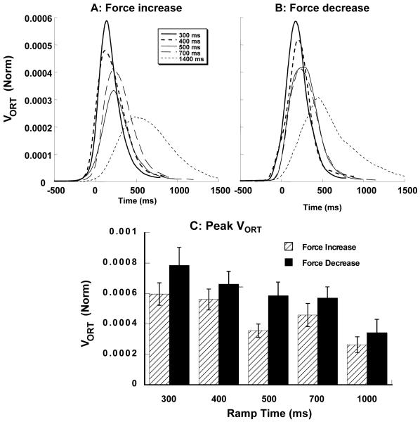
In contrast to V_UCM, V_ORT exhibited a bell-shaped time profile for both force increase and force decrease ramps. The peak of V_ORT was approximately half way through the ramp time, approximately coinciding with peak force rate. Patterns of time profiles of V_ORT for various conditions, averaged across subjects, are presented in Figures 5A and 5B for the force increase and force decrease ramps. Figure 5C shows that peak V_ORT increased as the ramp-time decreased. V_ORT is also higher for the force decrease segments as compared to the force increase segments. These observations were confirmed by a two-way repeated measures ANOVA performed on peak V_ORT with factors Ramp-Time (5 levels) and Direction (2 levels). Significant main effects were found for Ramp-Time (F _{(4, 63)} = 13.31, p < 0.001) and Direction (F _{(1, 63)} = 15.50, p < 0.001), but not for the interaction. Pair-wise comparisons showed that peak V_ORT for the 1400 ms ramp time was significantly different from peak V_ORT for all other conditions, peak V_ORT for the 700 ms ramp time was significantly different from that for the 300 ms ramps, peak V_ORT for 500 ms ramp time was significantly different from that for the 300 ms ramp. The effect of Direction was due to the higher V_ORT for the force decrease ramps as compared to the force increase ramps.

Figure 5.

Variance orthogonal to the UCM, V_ORT averaged across subjects for the force increase ramps (A) and force decrease ramps (B). C: Peak V_ORT for the different ramp times and two directions of force change. Averaged across subjects data with standard error bars are shown. The values were normalized by MVC squared and by the number of dimensions within the ORT sub-space. Note that V_ORT shows a bell-shaped profile; it increases for faster tasks.

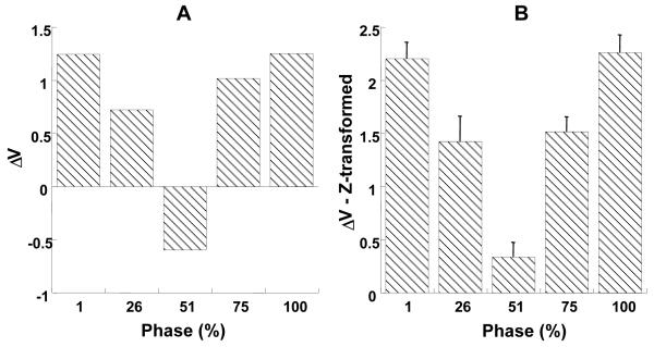
The index of mode co-variation, ΔV was higher in the beginning of the ramp and at the end of the ramp when compared with the middle portion of the ramp. Figure 6A shows a plot of ΔV, averaged across tasks and subjects for the selected five phases of force increase. Figure 6B shows a plot of log-transformed ΔV values, ΔV_z, averaged across tasks and subjects for various phases of force increase. The error bars show standard errors across subjects. A repeated measures ANOVA on ΔV_z with factors Ramp-time (5 levels), Direction (2 levels) and Phase (5 levels) showed significant main effect of Phase (F_(4,343) = 375, p < 0.001) but not of Ramp-time. Higher ΔV in the beginning of the trial and at the end of the trial when compared with the middle of the trial was confirmed by pair-wise comparisons. The interaction Direction × Phase was also significant (F_(4,343) = 77.21, p < 0.001). The interaction reflected a higher change of ΔV across various phases of the trial during force increase than during force decrease. The interaction Ramp-time × Phase was also significant (F _(16,343) =7.77, p<0.001).

Figure 6.

A: The index of mode co-variation, ΔV, B: Z-transformed values of ΔV (with standard error bars) at selected phases for the force increase ramps, averaged across subjects and tasks.

As post-hoc contrasts, we used two-way ANOVAs run separately on the data for the two ramp directions, force increase and force decrease. ANOVA on ΔV for force increase with factors Ramp-time and Phase showed a significant effect of Phase (F_(4,168) = 167.9, p < 0.001). This corresponded to a higher ΔV at the beginning and at the end of the trial when compared to the middle of the trial. The interaction Ramp-time × Phase was also significant (F_(4,168)=3.1, p<0.001). This was because ΔV was lower at the end of the trial when compared to the beginning of the task in faster tasks. But ΔV was higher at the end of the trial when compared to the beginning of the trial in slower tasks.

ANOVA on ΔV for force decrease with factors Ramp-time and Phase showed a significant effect of Phase (F_(4,168) = 275.87, p < 0.001). This corresponded to a higher ΔV at the beginning and at the end of the trial when compared to the middle of the trial. The interaction Ramp-time×Phase was also significant (F_(16,168) = 7.94, p < 0.001). This was because the difference in ΔV between the start of the trial and the end of the trial was lower in slower tasks than in faster tasks.

Relationships between characteristics of total force and components of variance

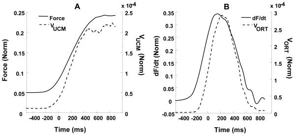
The two components of variance, V_UCM and V_ORT, showed time profiles similar to those of total force and force rate (dF/dt), respectively. These relationships are illustrated in Figure 6 for the force increase ramp over 400 ms performed by a typical subject. Figure 7A presents total force averaged across trials and V_UCM while Figure 7B presents mean dF/dt and V_ORT. Note the qualitative similarity between the curves shown in Figures 7A and 7B. This similarity suggested using a linear model described in the Methods (equation 8) to link the two variance components to total force characteristics. Table 1 presents the averages and standard errors of various parameters of this analysis. On average, the regressions accounted for more than 85% of the variance.

Figure 7.

A: Mean force (normalized by MVC) and V_UCM (normalized by MVC squared, per dimension in the UCM space) for a typical subject for one force increase condition (ramp time 500 ms). B: Mean force rate (normalized by MVC/s) and V_ORT (normalized by MVC squared) for the same subject and task. Note the similar time profiles.

Table 1.

Results of Regression Analysis

Ramp time	300 ms	400 ms	500 ms	700 ms	1400 ms
VUCM, force increase
a1 (×10−3)	2.27±0.79	7.15±4.99	6.4±4.42	7.15±5.69	5.46±3.24
c1(×10−4)	0.15±0.45	−2.74±2.36	−1.76±1.60	−3.12±2.85	−1.45±1.02
VUCM, force decrease
a1(×10−3)	2.21±0.58	4.77±2.92	3.44±1.88	3.62±2.52	3.81±2.14
c1(×10−5)	−1.02±3.74	−14.57±10.37	−5.51±7.78	−10.71±10.14	−5.21±5.57
VORT, force increase
a2(×10−4)	3.55±0.73	3.69±.77	1.21±0.43	2.91±0.76	2.08±0.4
b2(×10−4)	8.48±0.81	8.9±0.97	6.62±0.76	8.73±1.3	9.42±1.6
c2(×10−5)	−4.2±0.7	−4.3±0.8	−2.1±0.4	−3.9±0.8	−3.2±0.6
VORT, force decrease
a2(×10−4)	−1.03±0.72	−3.71±0.73	−1.84±0.71	−2.19±0.55	−2.96±0.75
b2(×10−4)	10.95±1.62	9.33±1.1	9.64±1.53	9.37±1.29	10.06±2.15
c2(×10−5)	1.34±1.61	6.35±1.67	2.29±1.44	3.05±1.14	5.75±1.7

Mean (± SEM) of the coefficients in the regression analyses of V_UCM and V_ORT using Eq. (8) over different ramp times. All fits were highly significant. No consistent change in any of the parameters was observed across conditions.

Within the equation V_UCM = a₁F_TOT + c₁, parameter a₁ did not vary consistently with ramp time, while the intercept c₁ was typically close to zero.

Within the equation V_ORT = a₂F_TOT + b₂dF/dt + c₂, parameter a₂ was relatively small and showed no regular trend with changes in ramp time. Parameter b₂ reflected the dependence of V_ORT on absolute force rate. This parameter also did not show any regular trend with ramp-time. Intercept c₂ was typically very small (close to zero).

A two-way repeated measures ANOVA was performed on parameter b₂ with factors Ramp-Time (5 levels) and Direction (2 levels). None of the effects were significant.

Links to Goodman et al. (2005) model

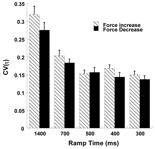
A model proposed by Goodman et al. (2005) specifies two scaling parameters, an amplitude parameter b and a timing parameter τ that modify a template u_n(t). Within this model, V_ORT is primarily defined by variance of τ, Var(τ). The coefficient of variation of the timing parameter τ was computed to check if this parameter varied systematically with ramp time. Figure 8 presents the average values of CV(τ) for various conditions. Error bars indicate standard errors. A two-way repeated measures ANOVA on CV(τ) with factors Ramp-time (5 levels) and Direction (2 levels) was performed. Significant main effects were found for Ramp-Time (F _{(4, 63)} = 66.28, p < 0.001) and Direction (F _{(1, 63)} = 7.83, p < 0.01), but not for the interaction. Pair-wise comparisons showed that CV(τ) values for ramp times 1400 ms and 700 ms were significantly different from those for all other ramp times. The effect of Ramp-Time corresponded to a decrease in CV(τ) as the ramp time decreased. In other words, as slope increased, CV(τ) decreased. The effect of Direction corresponded to a higher CV(τ) for force increase as compared to force decrease.

Figure 8.

CV(τ) for the force increase (dashed bars) and force decrease (black bars) for different ramp times. The plotted values are averages across subjects with standard error bars. CV(τ) decreases as ramp times decrease.

Anticipatory Synergy Adjustments

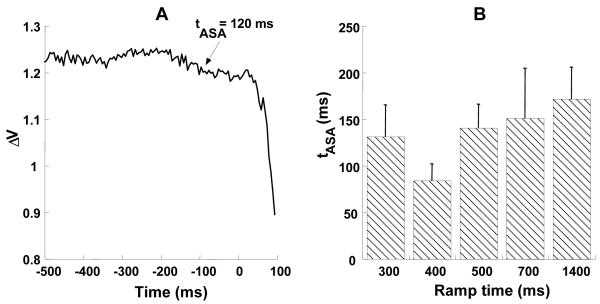
For this analysis, individual trials were aligned by the time at which the force rate reached 5% of its peak value. Then, an index of mode co-variation, ΔV was computed (See Methods). Figure 9A shows time-series of ΔV for a typical subject for the 400 ms ramp-time. Note that ΔV starts to decrease at about 120 ms before t₀.The time at which ASAs emerge (t_ASA) was computed for each ramp time for each subject. These times, averaged across subjects are presented in Figure 9B. The figure shows that t_ASA ranged from about 80 ms to about 180 ms; there was no consistent change in t_ASA with ramp time or direction. The magnitude of ASAs, ΔΔV_Z was (mean ± SE) 0.23±0.04 for force increase and 0.25±0.04 for force decrease. The index ΔΔV_Z did not show any consistent change with respect to ramp times or direction. This was confirmed by a two-way repeated measures ANOVA on ΔΔV_Z with factors Ramp-time (5 levels) and Direction (2 levels). There were no significant effects.

Figure 9.

A: A typical time profile of ΔV showing a decrease in ΔV that starts about 120 ms before force change initiation (t₀). B: Time of ASA initiation (t_ASA) as a function of ramp time. Averages across subjects with standard error bars are presented. t_ASA shows no consistent change across ramp times.

Discussion

The main question asked in our study was whether the controller was able to prevent the “bad variance”, V_ORT from increasing with the force rate as observed in the previous study of cyclic force production tasks (Friedman et al. 2009). We got a negative answer: A drop in force ramp time was associated with an increase in total force variance (and V_ORT) unlike the results of the cited study of cyclic tasks. However, analysis of the data within the Goodman model (Goodman et al. 2005) documented significant adjustments in variability of the timing parameter τ, similarly to the observations in the study of cyclic force production. We will discuss implications of these seemingly contradictory findings for the control of discrete and cyclic actions.

Our secondary goal was to explore quantitative characteristics of anticipatory synergy adjustments (ASAs) with changes in the force rate. We expected to see earlier and larger ASAs prior to trials with faster force production. This prediction was not supported by the data. Indeed, ASAs were seen prior to the initiation of force change in all the tasks, but both the timing and magnitude of ASAs were similar across tasks with different force rates. This forced us to reconsider the earlier hypothesis on the role of ASAs in preparation to an action (cf. Olafsdottir et al. 2005; Shim et al. 2005).

Components of force variance in redundant tasks

Motor redundancy may be viewed as a source of computational problems that require using sophisticated methods, for example optimization (for review see Seif-Naraghi and Winters 1990; Rosenbaum et al. 2001), to find particular solutions from the infinite sets afforded by redundant systems. A different view is represented by the principle of abundance (Gelfand and Latash 1998). According to this approach, when a neural controller faces a problem of motor redundancy, it does not look for unique solutions but rather facilitates families of solutions that are equally capable of solving the problem. Within this general framework, the uncontrolled manifold (UCM) hypothesis offers a computational approach, which we used to analyze across-trials variance in two sub-spaces of elemental variables (finger modes, see Danion et al. 2003), compatible with the total force magnitude (estimated as the average magnitude across trials) and leading to total force changes. We address these two variance components as “good” and “bad” variance or, equivalently, as V_UCM and V_ORT.

In this study, we observed multi-finger synergies stabilizing the total force (V_UCM > V_ORT) across all the tasks (similarly to earlier studies, Latash et al. 2002a; Shim et al. 2005). Changes in the force rate led to significant changes in only one of the two variance components, V_ORT, resulting in smaller differences between V_UCM and V_ORT for faster actions (reflected in the smaller synergy index values, ΔV). Force direction also had an effect on V_ORT, while V_UCM was similar between the force-up and force-down tasks: Force-down tasks were associated with larger V_ORT reflected in the larger total force variance. These results confirm the findings of Shim et al. (2005) who studied tasks with trapezoidal time profiles of force production.

We used an earlier suggested regression model (Latash et al. 2002a) linking the two variance components to force and force rate (dF/dt) magnitudes. Within this model, V_ORT is linearly linked to dF/dt. Although the linear relationships between V_ORT and dF/dt were seen in this study, as well as in the earlier study of cyclic force production (Friedman et al. 2009), the regression coefficients (b₂) in the two studies behaved differently. During cyclic force production, speeding the action up resulted in a significant drop in the regression coefficient such that V_ORT modulation with dF/dt was present within each task but not across task frequencies. This was due to adjustments of the regression coefficient to action frequency that exactly cancelled out the expected increase in V_ORT with the increase in dF/dt in faster actions. In the present study of discrete actions, V_ORT was modulated with dF/dt both within and across tasks, and there was no adjustment of the regression coefficient across tasks performed at different speeds.

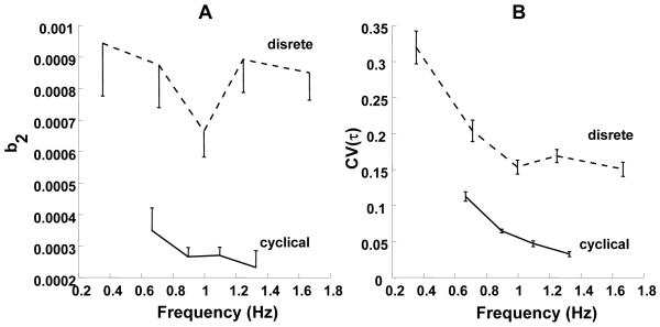
These differences are illustrated in Figure 10A that shows changes in the b₂ regression coefficient across different action frequencies. For discrete tasks, we estimated the action frequency assuming that the ramp time corresponded approximately to a half-cycle duration. Note that in this study we explored a broader range of ramp times (frequencies), and no adjustments in b₂ were observed across frequencies.

Figure 10.

A: Plots of the regression coefficient b₂ for both cyclical and discrete tasks. While b₂ decreases with an increase in action frequency in cyclical tasks, it does not show a consistent change in discrete tasks. B: CV(τ) as a function of frequency for both cyclical and discrete tasks. As frequency increases, CV(τ) decreases in both discrete and cyclical tasks. The data for the cyclical tasks are from Friedman et al. 2009.

Why does speeding the action up lead to an increase in V_ORT magnitude in the discrete but not in cyclic tasks? To address this issue we turn to a model of multi-finger force production developed earlier by Goodman and colleagues (Goodman et al. 2005).

Timing errors: Similarities and differences between discrete and cyclic actions

There have been several attempts to model typical patterns of finger force (and finger mode) variance observed in multi-finger force production tasks. These attempts involved optimal feedback control (Todorov and Jordan 2002), central back-coupling (Latash et al. 2005), and feed-forward control schemes (Goodman and Latash 2006). One of these approaches extended an earlier model by Goodman (Gutman) and his colleagues of single-joint kinematic variability (Gutman et al. 1993) to multi-finger force production. This model, described briefly in Methods, is based on two main parameters, b and τ, related to adjustments of action magnitude and speed. The model assumes that, for each particular trial, both parameters are selected from normally distributed sets that can be characterized with variances Var(b) and Var(τ). According to the model, the “bad” variance is primarily defined by Var(τ).

Figure 10B shows changes in the coeffcient of variation of τ, CV(τ), across the two studies with cyclic and discrete force production tasks. Note the much higher CV(τ) values for the discrete tasks. In both studies, CV(τ) changed with action frequency. It can be seen from this figure, however, that the drop in CV(τ) with frequency was faster for the cyclic tasks. Fitting the data with logarithmic functions produces: CV(τ) = 0.17848 - 0.217log(f); R = 0.953 for the discrete actions, and CV(τ) = 0.060298 - 0.267log(f); R = 0.989 for the cyclic actions, where f stands for frequency. Note the larger regression coefficient for the cyclic actions. The faster drop in CV(τ) in cyclic tasks was associated with significant adjustments in b₂ that allowed the system to maintain constant total force variance across tasks. In discrete tasks, the smaller CV(τ) adjustment was insufficient to cause b₂ adjustments, and total force variance increased with a decrease in action time (increase in action frequency).

Our findings fit a general theoretical view that the neural control of cyclic tasks may involve adjustments in fewer control parameters (Hogan, Sternad 2007; Ronsse et al. 2009). In the dynamic systems parlance, control of a cyclic task may be associated with setting a limit cycle attractor with constant parameters, while the control of discrete actions involves transition between two point attractors at a controlled rate that has to be defined for each such transition. This general view has been supported by findings suggesting that neural implementation of cyclic and discrete motor tasks may be different (Schaal et al. 2004; Spencer et al. 2007).

We should, however, mention a recent publication that reported better timing accuracy in discrete tasks as compared to cyclic tasks (Elliott et al. 2009). This study, however, differed from our experiments in a major aspect: It involved tapping tasks under different instructions including continuous sine-like force production and discrete taps that were still produced rhythmically. This is a major difference from our tasks, where there was no rhythm underlying the production of discrete force ramps. Also, the emphasis of the Elliott et al. study was on timing accuracy, not force magnitude accuracy.

What is the role of anticipatory synergy adjustments?

Several earlier studies reported changes in the index (ΔV) of force stabilizing multi-finger synergies 100-150 ms prior to the earliest signs of force change in anticipation of a fast voluntary force change (Olafsdottir et al. 2005; Shim et al. 2005) and in anticipation of a self-triggered force perturbation (Kim et al. 2006; Shim et al. 2006). These phenomena have been termed anticipatory synergy adjustments (ASAs). Some of the features of ASAs suggest rather direct parallels with the well known anticipatory postural adjustments (APAs, reviewed in Massion 1992). Such features involve the similar timing of both adjustments, their changes under simple reaction time instruction, and attenuation with healthy aging (Inglin and Woollacott 1988; De Wolf et al. 1998; Olafsdottir et al. 2005, 2007).

In our study, we observed ASAs within about the same time interval as in earlier studies, 80-200 ms prior to the first detectable change in total force. A surprising result was the presence of ASAs prior to very slow force ramps that were similar in both time and magnitude characteristics to the ASAs observed prior to the fastest tasks. An earlier hypothesis linked ASAs to attenuation of a synergy that would act against a planned quick force change (Olafsdottir et al. 2005). Our results suggest that the controller does not distinguish among force changes at different rates when it facilitates ASAs. Note that APAs in the leg/trunk muscles prior to fast arm movements scale both their timing and magnitude with the planned action speed and may even disappear prior to slow actions (Horak et al. 1984; Crenna et al. 1987). The current finding seems to be the first one to report a qualitative difference in the behaviors of ASAs and APAs.

The lack of the difference in ASA characteristics across tasks with different ramp times may be in part due to a common feature of these tasks, that is early small-amplitude, poorly reproducible force jumps that are very hard to avoid even if one plans a smooth and slow force increase. Such early force jumps are reflected in a disproportionate transient increase in “bad variance” of finger force reported over the first 100-200 ms after the initiation of force production (Shim et al. 2003, 2005). The current results suggest that ASAs are poorly graded with planned action speed and represent relatively standard synergy adjustments to planned changes in performance variables produced by redundant sets of effectors.

Concluding comments

According to a general scheme suggested by Schöner (2002), movement production involves a multi-level hierarchical system. Two levels of this scheme are those of timing (when to do an action and how quickly to do it) and of synergies (how to organize elemental variables such that they stabilize important features of performance). According to this scheme, if there are timing errors originating from the higher timing level, they cannot be corrected at the lower synergy level.

In our study, variance of τ has been assumed to reflect variance at the hypothetical timing level of the Schöner scheme. This variance is indeed reflected primarily in the “bad” variance at the level of individual fingers; in other words, the co-variation organized at the synergy level is unable to handle errors introduced by this variance. The difference between the discrete and cyclic tasks suggests, however, that the controller is able to mitigate the effects of varied τ on performance only for cyclic tasks but not for discrete ones. This is likely to originate from two sources of the observed τ variance. First, for an ongoing cyclic task, there is variance of τ across cycles that reflects different values taken from the same distribution. Second, if a task is to be stopped and repeated, the new realization is associated with specifying a new distribution of τ and selecting a value from that distribution.

In other words, τ variance in discrete tasks reflects two sources of variance, between distributions of τ for different task realizations and within-a-distribution variance. The within-a-distribution variance is common across the cyclic and discrete tasks. Our results suggest that the controller is able to adjust to this τ variance component by changing the coefficient that links “bad” variance and force rate. This is likely true for both rhythmic and discrete tasks. The controller, however, seems unable to handle the between-distributions source of τ variance that dominates force variance in discrete tasks and leads to the described qualitative difference between the discrete and cyclic tasks.

References

- Christou EA, Grossman M, Carlton LG. Modeling variability of force during isometric contractions of the quadriceps femoris. J Mot Behav. 2002;34:67–81. doi: 10.1080/00222890209601932. [DOI] [PubMed] [Google Scholar]
- Crenna P, Frigo C, Massion J, Pedotti A. Forward and backward axial synergies in man. Exp Brain Res. 1987;65:538–548. doi: 10.1007/BF00235977. [DOI] [PubMed] [Google Scholar]
- De Wolf S, Slijper H, Latash ML. Anticipatory postural adjustments during self-paced and reaction-time movements. Exp Brain Res. 1998;121:7–19. doi: 10.1007/s002210050431. [DOI] [PubMed] [Google Scholar]
- Danion F, Schöner G, Latash ML, Li S, Scholz JP, Zatsiorsky VM. A force mode hypothesis for finger interaction during multi-finger force production tasks. Biol Cybern. 2003;88:91–98. doi: 10.1007/s00422-002-0336-z. [DOI] [PubMed] [Google Scholar]
- Elliott MT, Welchman AE, Wing AM. Being discrete helps keep to the beat. Exp Brain Res. 2009;192:731–737. doi: 10.1007/s00221-008-1646-8. [DOI] [PubMed] [Google Scholar]
- Friedman J, SKM V, Zatsiorsky VM, Latash ML. The sources of two components of variance: An example of multifinger cyclic force production tasks at different frequencies. Exp Brain Res. 2009;196:263–277. doi: 10.1007/s00221-009-1846-x. [DOI] [PMC free article] [PubMed] [Google Scholar]
- Gelfand IM, Latash ML. On the problem of adequate language in movement science. Motor Control. 1998;2:306–313. doi: 10.1123/mcj.2.4.306. [DOI] [PubMed] [Google Scholar]
- Goodman SR, Latash ML. Feedforward control of a redundant motor system. Biol Cybern. 2006;95:271–280. doi: 10.1007/s00422-006-0086-4. [DOI] [PubMed] [Google Scholar]
- Goodman SR, Shim JK, Zatsiorsky VM, Latash ML. Motor variability within a multi-effector system: Experimental and analytical studies of multi-finger production of quick force pulses. Exp Brain Res. 2005;163:75–85. doi: 10.1007/s00221-004-2147-z. [DOI] [PMC free article] [PubMed] [Google Scholar]
- Gutman SR, Latash ML, Gottlieb GL, Almeida GL. Kinematic description of variability of fast movements: Analytical and experimental approaches. Biol Cybern. 1993;69:485–492. [PubMed] [Google Scholar]
- Hogan N, Sternad D. On rhythmic and discrete movements: reflections, definitions and implications for motor control. Exp Brain Res. 2007;181:13–30. doi: 10.1007/s00221-007-0899-y. [DOI] [PubMed] [Google Scholar]
- Horak FB, Esselman PE, Anderson ME, Lynch MK. The effects of movement velocity, mass displaced and task certainty on associated postural adjustments made by normal and hemiplegic individuals. J Neurol Neurosurg Psychiat. 1984;47:1020–1028. doi: 10.1136/jnnp.47.9.1020. [DOI] [PMC free article] [PubMed] [Google Scholar]
- Inglin B, Woollacott MH. Anticipatory postural adjustments associated with reaction time arm movements: a comparison between young and old. J Gerontol. 1988;43:M105–M113. doi: 10.1093/geronj/43.4.m105. [DOI] [PubMed] [Google Scholar]
- Kilbreath SL, Gandevia SC. Limited independent flexion of the thumb and fingers in human subjects. J Physiol. 1994;479:487–497. doi: 10.1113/jphysiol.1994.sp020312. [DOI] [PMC free article] [PubMed] [Google Scholar]
- Kim SW, Shim JK, Zatsiorsky VM, Latash ML. Anticipatory adjustments of multi-finger synergies in preparation for self-triggered perturbations. Exp Brain Res. 2006;174:604–612. doi: 10.1007/s00221-006-0505-8. [DOI] [PubMed] [Google Scholar]
- Latash ML. Stages in learning motor synergies: A view based on the equilibrium-point hypothesis. Hum Move Sci. 2010a doi: 10.1016/j.humov.2009.11.002. in press. [DOI] [PMC free article] [PubMed] [Google Scholar]
- Latash ML. Motor synergies and the equilibrium-point hypothesis. Motor Control. 2010b doi: 10.1123/mcj.14.3.294. in press. [DOI] [PMC free article] [PubMed] [Google Scholar]
- Latash ML, Friedman J, Kim SW, Feldman AG, Zatsiorsky VM. Prehension synergies and control with referent hand configurations. Exp Brain Res. 2010;202:213–229. doi: 10.1007/s00221-009-2128-3. [DOI] [PMC free article] [PubMed] [Google Scholar]
- Latash ML, Scholz JF, Danion F, Schöner G. Finger coordination during discrete and oscillatory force production tasks. Exp Brain Res. 2002a;146:412–432. doi: 10.1007/s00221-002-1196-4. [DOI] [PubMed] [Google Scholar]
- Latash ML, Scholz JP, Schöner G. Motor control strategies revealed in the structure of motor variability. Exerc Sport Sci Rev. 2002b;30:26–31. doi: 10.1097/00003677-200201000-00006. [DOI] [PubMed] [Google Scholar]
- Latash ML, Scholz JP, Schöner G. Toward a new theory of motor synergies. Motor Control. 2007;11:276–308. doi: 10.1123/mcj.11.3.276. [DOI] [PubMed] [Google Scholar]
- Latash ML, Shim JK, Smilga AV, Zatsiorsky V. A central back-coupling hypothesis on the organization of motor synergies: a physical metaphor and a neural model. Biol Cybern. 2005;92:186–191. doi: 10.1007/s00422-005-0548-0. [DOI] [PMC free article] [PubMed] [Google Scholar]
- Massion J. Movement, posture and equilibrium – interaction and coordination. Prog Neurobiol. 1992;38:35–56. doi: 10.1016/0301-0082(92)90034-c. [DOI] [PubMed] [Google Scholar]
- Newell KM, Carlton LG. Force variability in isometric responses. J Exp Psychol: Hum Percept Perform. 1993;14:37–44. [PubMed] [Google Scholar]
- Olafsdottir H, Yoshida N, Zatsiorsky VM, Latash ML. Anticipatory covariation of finger forces during self-paced and reaction time force production. Neurosci Lett. 2005;381:92–96. doi: 10.1016/j.neulet.2005.02.003. [DOI] [PMC free article] [PubMed] [Google Scholar]
- Olafsdottir H, Yoshida N, Zatsiorsky VM, Latash ML. Elderly show decreased adjustments of motor synergies in preparation to action. Clin Biomech. 2007;22:44–51. doi: 10.1016/j.clinbiomech.2006.08.005. [DOI] [PMC free article] [PubMed] [Google Scholar]
- Rosenbaum DA, Meulenbroek RJ, Vaughan J, Jansen C. Posture-based motion planning: applications to grasping. Psychol Rev. 2001;108:709–734. doi: 10.1037/0033-295x.108.4.709. [DOI] [PubMed] [Google Scholar]
- Ronsse R, Sternad D, Lefèvre P. A computational model for rhythmic and discrete movements in uni- and bimanual coordination. Neural Comput. 2009;21:1335–1370. doi: 10.1162/neco.2008.03-08-720. [DOI] [PMC free article] [PubMed] [Google Scholar]
- Schaal S, Sternad D, Osu R, Kawato M. Rhythmic arm movement is not discrete. Nat Neurosci. 2004;7:1136–1143. doi: 10.1038/nn1322. [DOI] [PubMed] [Google Scholar]
- Scholz JP, Schöner G. The uncontrolled manifold concept: Identifying control variables for a functional task. Exp Brain Res. 1999;126:289–306. doi: 10.1007/s002210050738. [DOI] [PubMed] [Google Scholar]
- Schöner G. Timing, clocks, and dynamical systems. Brain Cognition. 2002;48:31–51. doi: 10.1006/brcg.2001.1302. [DOI] [PubMed] [Google Scholar]
- Seif-Naraghi AH, Winters JM. Optimized strategies for scaling goal-directed dynamic limb movements. In: Winters JM, Woo SL-Y, editors. Multiple Muscle Systems. Biomechanics and Movement Organization. Springer-Verlag; New York: 1990. pp. 312–334. [Google Scholar]
- Shim JK, Latash ML, Zatsiorsky VM. The central nervous system needs time to organize task-specific covariation of finger forces. Neurosci Lett. 2003;353:72–74. doi: 10.1016/j.neulet.2003.08.079. [DOI] [PubMed] [Google Scholar]
- Shim JK, Olafsdottir H, Zatsiorsky VM, Latash ML. The emergence and disappearance of multi-digit synergies during force production tasks. Exp Brain Res. 2005;164:260–270. doi: 10.1007/s00221-005-2248-3. [DOI] [PMC free article] [PubMed] [Google Scholar]
- Shim JK, Park J, Zatsiorsky VM, Latash ML. Adjustments of prehension synergies in response to self-triggered and experimenter-triggered load and torque perturbations. Exp Brain Res. 2006;175:641–653. doi: 10.1007/s00221-006-0583-7. [DOI] [PMC free article] [PubMed] [Google Scholar]
- Shinohara M, Li S, Kang N, Zatsiorsky VM, Latash ML. Effects of age and gender on finger coordination in maximal contractions and submaximal force matching tasks. J Appl Physiol. 2003;94:259–270. doi: 10.1152/japplphysiol.00643.2002. [DOI] [PubMed] [Google Scholar]
- Shinohara M, Scholz JP, Zatsiorsky VM, Latash ML. Finger interaction during accurate multi-finger force production tasks in young and elderly persons. Exp Brain Res. 2004;156:282–292. doi: 10.1007/s00221-003-1786-9. [DOI] [PubMed] [Google Scholar]
- Slifkin AB, Newell KM. Noise, information transmission, and force variability. J Exp Psychol: Hum Percept Perform. 1999;25:837–851. doi: 10.1037//0096-1523.25.3.837. [DOI] [PubMed] [Google Scholar]
- Spencer RMC, Verstynen T, Brett M, Ivry R. Cerebellar activation during discrete and not continuous timed movements: an fMRI study. NeuroImage. 2007;36:378–387. doi: 10.1016/j.neuroimage.2007.03.009. [DOI] [PMC free article] [PubMed] [Google Scholar]
- Sternad D, Dean WJ. Rhythmic and discrete elements in multi-joint coordination. Brain Res. 2003;989:152–171. doi: 10.1016/s0006-8993(03)03292-x. [DOI] [PubMed] [Google Scholar]
- Todorov E, Jordan MI. Optimal feedback control as a theory of motor coordination. Nature Neurosci. 2002;5:1226–1235. doi: 10.1038/nn963. [DOI] [PubMed] [Google Scholar]
- Zatsiorsky VM, Li ZM, Latash ML. Coordinated force production in multi-finger tasks: Finger interaction and neural network modeling. Biol Cybern. 1998;79:139–150. doi: 10.1007/s004220050466. [DOI] [PubMed] [Google Scholar]
- Zatsiorsky VM, Li ZM, Latash ML. Enslaving effects in multi-finger force production. Exp Brain Res. 2000;131:187–195. doi: 10.1007/s002219900261. [DOI] [PubMed] [Google Scholar]