

Abstract
This is the second article in a series of three studies that investigate the anatomical determinants of thalamocortical (TC) input to excitatory neurons in a cortical column of rat primary somatosensory cortex (S1). Here, we report the number and distribution of NeuN-positive neurons within the C2, D2, and D3 TC projection columns in P27 rat somatosensory barrel cortex based on an exhaustive identification of 89 834 somata in a 1.15 mm3 volume of cortex. A single column contained 19 109 ± 444 neurons (17 560 ± 399 when normalized to a standard-size projection column). Neuron density differences along the vertical column axis delineated “cytoarchitectonic” layers. The resulting neuron numbers per layer in the average column were 63 ± 10 (L1), 2039 ± 524 (L2), 3735 ± 905 (L3), 4447 ± 439 (L4), 1737 ± 251 (L5A), 2235 ± 99 (L5B), 3786 ± 168 (L6A), and 1066 ± 170 (L6B). These data were then used to derive the layer-specific action potential (AP) output of a projection column. The estimates confirmed previous reports suggesting that the ensembles of spiny L4 and thick-tufted pyramidal neurons emit the major fraction of APs of a column. The number of APs evoked in a column by a sensory stimulus (principal whisker deflection) was estimated as 4441 within 100 ms post-stimulus.
Keywords: cortex layer, neuron density, POm, somatosensory barrel cortex, VPM
Introduction
The trigeminal system of rodents is unique in its discrete one-to-one relationship between individual whiskers and cortical barrel columns. For building mechanistic models of cortical columns, or making quantitative predictions about their functional properties, it is a crucial prerequisite to provide precise numbers on the spatial dimensions of cortical columns and the number of neurons in all layers of a column.
In the preceding article, we have quantified the dimensions of thalamocortical (TC) projections originating in the ventral posteromedial (VPM) and the medial part of the posterior group (POm) thalamic nuclei (Wimmer et al. 2010). This allowed the definition of an anatomical “projection column.” The dimensions of such a projection column were approximated by a cylindroid with a height of approximately 1840 μm and a cross-sectional area of approximately 121 000 μm2 (Wimmer et al. 2010). In this article, we aimed at counting the number of neurons in such a projection column. Together with the data on TC projections, these numbers are then used to compute the average TC innervation of excitatory neurons in a cortical column as presented in the subsequent article (Meyer et al. 2010).
The number of neurons in a cortical column has been previously estimated by extrapolations based on measurements of neuron density (sampled using Sterio’s disector method; Sterio 1984). However, the estimates for neuron density in rat somatosensory cortex varied by almost a factor of 2: between 48 000 per cubic millimeter (Beaulieu 1993) and 77 000 per cubic millimeter (Keller and Carlson 1999). To obtain more precise measurements that will allow a quantitative interpretation of the data on neuron numbers, we therefore aimed at counting the number of neurons in an entire TC projection column. It was first necessary to precisely count at least one complete column to exclude fixation and sampling artifacts. This is reported in the present study for the C2 and D2 barrel columns in a P27 rat. In addition, we used an automated counting method (Oberlaender et al. 2009) calibrated by the manual counts to evaluate a third data set comprising the D3 column from the same animal.
We labeled neuronal nuclei and the surrounding cytosol by the neuron-specific nuclear protein “Neuronal Nuclei” (NeuN; Mullen et al. 1992) in serial sections of the barrel field cut in the tangential plane. These stainings were combined with viral expression of a fluorescent protein in TC axons (Wimmer et al. 2004, 2010) to delineate the TC projection column. Together, this allowed to measure the number of neurons in a TC projection column by complete manual counting. We used the vertical cell density profile to quantitatively define layer borders and measured the number of neurons that constitute particular cytoarchitectonic layers of a projection column. Finally, the data on neuron numbers in the cytoarchitectonically defined cortical layers of a cortical column were used to estimate the “action potential (AP) budget” of a single cortical column following a deflection of the principal whisker (de Kock et al. 2007).
Materials and Methods
Preparation
All experimental procedures were performed in accordance with the German Animal Welfare Act.
The methods used for virus delivery were the same as described before (Wimmer et al. 2004, 2010). Briefly, male P24 Wistar rats (40–60 g body weight) were anaesthetized by intraperitoneal injection of 5 μg/kg fentanyl, 2 mg/kg midazolam, and 150 μg/kg medetomidine. Adeno-associated virus (AAV)–mOrange (100–200 nL; 3 × 10⁶ infectious particles/mL) was stereotaxically injected into VPM using calibrated injection capillaries. The injection coordinates were as follows (in mm): 2.85 posterior of bregma, 3.2 lateral of the midline, and 5.05 deep from the pia. VPM-injected animals were perfused 11 days after injection.
For removal of tissue for immunohistochemistry, rats were euthanized and perfused transcardially with 1 mL/g body weight of 100 mM sodium phosphate buffer (NaH2PO4/Na2HPO4), pH 7.2 (PB), followed by 1 mL/g body weight of PB containing 4% paraformaldehyde (PFA). The animal used for neuron counting in the C2, D2, and D3 columns (right cerebral hemisphere) was male and 27 days old (body weight: 85 g). The brain was removed from the skull and postfixed in PB containing 4% PFA for 2–5 h. Tangential (for neuron counting) or semi-coronal (for comparison of GAD67 labeling and VPM axon projections) slices of 50 μm thickness were cut in PB using a vibrating microslicer (Slicer HR-2; Sigmann Elektronik). Semi-coronal slices were cut at an angle of 50° to the interhemispheric sulcus (measured counterclockwise for slicing right hemispheres) so that the slicing plane was approximately parallel to the barrel arcs, where inter-barrel distances are larger than within the barrel rows.
In vivo neuron recording and labeling were performed as described previously (de Kock et al. 2007).
Immunohistochemistry
Slices were double immunolabeled for the 67 kDa isoform of glutamate decarboxylase (GAD67) (Kaufman et al. 1986; Kobayashi et al. 1987; Julien et al. 1990) and neuron-specific nuclear protein (NeuN) (Mullen et al. 1992). Slices were permeabilized and blocked in 0.5% Triton X-100 (TX) (Sigma-Aldrich) in PB containing 4% normal goat serum (NGS) (Jackson ImmunoResearch Laboratories) for 2 h at room temperature. Primary antibodies (Chemicon) were diluted to 1:800 (mouse anti-GAD67, catalog number MAB5406) and 1:500 (mouse anti-NeuN, catalog number MAB377). They were incubated at 4 °C in PB containing 1% NGS for 40–48 h. Secondary antibodies (1:500 goat anti-mouse IgG2a Alexa 488; 1:500 goat anti-mouse IgG1 Alexa 647) were incubated at room temperature in PB containing 3% NGS and 0.3% TX for 2–3 h. Slices were mounted on slides, embedded with SlowFade Gold (Invitrogen), and enclosed with a coverslip.
Image Acquisition
Slices were imaged using BX51 (Olympus) and Axiovert 135 (Carl Zeiss AG) microscopes at a magnification of ×2.5 (numerical aperture [NA] 0.12) or ×4 (NA 0.10). A TCS SP5 confocal laser scanning microscope (Leica Microsystems) with a ×40 Leica (HCX PL APO CS; NA 1.25, oil immersion) objective was used to obtain image stacks of 1024 × 1024 pixel xy size from the different fluorescence channels. The effective voxel size was 0.366 × 0.366 × 0.610 μm3. Laser excitation wavelengths were 458 nm (Argon) for Alexa 488 and 633 nm (Helium–Neon) for Alexa 647. The wavelength selection windows were as follows: 495–550 nm for Alexa 488 and 640–720 nm for Alexa 647. Mosaic scanning with a scanning table (Märzhäuser) was used to scan up to 5 × 5 tiles (∼1875 × 1875 × 50 μm3) per slice.
Manual Placement of Soma Markers
The confocal image stacks were aligned manually in AMIRA 4.0 or 4.1 (Visage Imaging). Then, the optical sections parallel to the confocal scanning plane (x–y plane) of the NeuN fluorescence channel were examined, and 3D-markers were placed manually at the presumed “soma” center. The z-coordinate of a soma center was chosen as the z-coordinate of the optical section containing the largest cross section of the nucleus of a cell. If a cell was not completely located within a slice, it was counted only if the maximum soma diameter was contained in the slice (judged by either a successive increase and a decrease of the cross section size or by a constant cross section size for at least 3 successive optical sections). This ensured that only cells whose soma center was located within the slice were counted, thus eliminating edge effects.
Accuracy of Manual Counting
To determine the precision of the slicing and counting method, the following control experiments were made: 1) The inter-user variability of the counting algorithm was found to be small: in a region from L4 with a very high soma density, 3 observers counted 487 ± 2.1% neurons (range 478–498 neurons). 2) We checked that for consecutive slices, all cells at the slice borders could be recovered in the adjacent slice (for an example of 6 consecutive tangential slices, see inset in Fig. 3A) and that the selection criterion was mutually exclusive for the large majority of cells contained in 2 adjacent sections. 3) We simulated the effect of cutting somata by virtually cutting a 50-μm thick slice to 36 μm thickness (cutting off 7 μm at the top and bottom, respectively). Then, the resulting data set was counted. Next, the full-thickness slice was counted, and the resulting landmark set was cut to 36 μm thickness (again taking away 7 μm at the top and bottom, respectively). Both methods yielded comparable results (479 and 498 neurons, respectively, i.e., a 3.8% underestimation due to the slicing artifact). 4) For 35 consecutive slices containing the C2 column, 20% of the slice volume was cropped off the edge of each slice. The average ratio of the number of neurons contained in the cropped subvolume to the number of all neurons counted in the slice was 80.9 ± 5.0%. Assuming a homogeneous neuron density along the z-axis of each 50-μm thick slice, this also shows that our counting is not affected by edge effects.
Figure 3.

Definition of layer borders based on the density of NeuN-positive cell bodies along the vertical column axis. (A) Cytoarchitectonic layer borders (dashed black horizontal lines) determined based on the vertical neuron density gradients (red line, left panel) by fitting Gaussian functions to the neuron density z-profile of the C2 column at the presumed layer borders. Inset: Example of fit used to define the L4-to-L5A border. HWHM, half width half maximum. Maximum intensity projection images of 6 consecutive slices of the C2 column illustrating that the fitted L4-to-L5A layer border (green dashed line) matched the apparent density drop in the anti-NeuN immunofluorescence. For a summary of the resulting layer heights, see Table 2. (B) Comparison of the such defined layer borders with profiles of thalamic projection density (profiles from Meyer et al. 2010). *The border between L5A and L5B could not be defined based on changes in neuron density. We therefore used GAD67 immunofluorescence to delineate the border between L5A and L5B, which provided clear subdivision of layer 5 (cf. Fig. 1B) and matched the putative L5A outline defined by the POm projection density.
Accuracy of Automated Counting
For one of the columns analyzed in this report (the D3 column), we used an automated counting method that was calibrated by the manual counts (Oberlaender et al. 2009). For calibration, we compared the results of the automated counting in the C2 and D2 columns with the entirely manually counted results and found deviations of less than 3% for the whole-column counts and ∼6% as average absolute discrepancy at any depth from the pia (see Supplementary Fig. 1 for details of this comparison).
Layer Border Definition
Gaussian functions,  , were fitted to the peaks of the neuron density profile to delineate L2 from L3, L3 from L4, L5A from L4, L5B from L6A, and L6B from L6A in IgorPro 4.09 (Wavemetrics) with manually set c1, c2, and z0. Layer borders zlim were then defined as the depth zlim at half maximum:
  . At the L1-to-L2 border, the fit to the neuron density profile overestimated the width of L1 due to the sudden (within 10 μm) rise in neuron density at this border; this border was therefore defined by inspection of a high-resolution neuron density profile. The L5A-to-L5B border was defined by visual inspection of the GAD67 epifluorescence image.
Results
Definition of the Outlines of a TC Projection Column
We used the anatomically well-defined TC projections from the ventroposteromedial thalamic nucleus (VPM) as anatomical landmarks to define a cortical projection column. TC axons were labeled by virus-mediated fluorescence as reported in the preceding article (Wimmer et al. 2010). Figure 1A shows the fluorescence intensity of TC (VPM) projections in a semi-coronal slice from rat barrel cortex. The barrels in L4 are clearly discernible as areas of higher TC projection density. The circumference of the TC projection column in the horizontal plane was defined by the maximum outline of VPM projection intensity in L4. We incidentally found that immunolabeling of the 67 kDa isoform of glutamate decarboxylase (GAD67) permitted delineation of outlines that were well aligned to the column outlines defined by the labeling of TC axons (cf. Fig. 1A vs. Fig. 1B). GAD67 immunolabeling could thus be used for correlating the projection column outlines to the measurements of the number of neurons. This correspondence greatly facilitated the experiments because the labeling of TC axons was not needed for each of the experiments. A similar delineation of barrels in L4 was not found for simultaneous immunolabeling of both the 65 and the 67 kDa isoforms of GAD (data not shown). We did not further investigate the source of this labeling but used the outlines of the anti-GAD67 fluorescence intensity in L4 as surrogate labels to define the column outlines in tangential sections of barrel cortex for counting all neurons in a column (Fig. 1C,D).
Figure 1.
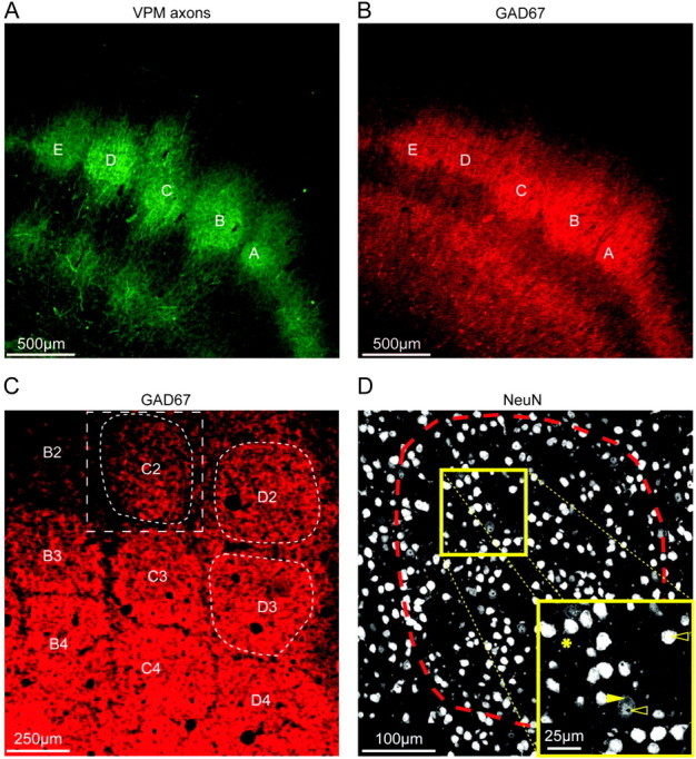
Outlines of TC projection columns. (A) Fluorescence image of a semi-coronal slice of barrel cortex showing thalamic VPM axons visualized by viral-mediated fluorescence (mOrange). Barrels A–E in layer 4 can be delineated as spots of high VPM axon density. (B) GAD67 immunofluorescence image of the slice shown in (A). The GAD67 immunofluorescence showed hot spots in layer 4 whose outlines match the patches of TC projection. (C) GAD67 fluorescence image of a tangential slice of L4 of barrel cortex. Arcs 2–4 of rows B–D are shown. Barrels can be delineated as hot spots of GAD67 immunofluorescence. The white box (dashed rectangle) illustrates the region of interest that was selected for imaging the C2 barrel column (dashed barrel outline) through the entire depth of the cortex using confocal scanning microscopy. The D2 and D3 barrel columns were also imaged. (D) NeuN immunofluorescence image (single optical slice) from a confocal scan of a tangential slice (thickness: 50 μm) of the region of interest outlined in (C). Dashed line: barrel outline of the C2 barrel. The inset illustrates that NeuN immunolabeling predominantly stains the nucleus. However, it also outlines the cytosol (arrows); sometimes, even parts of dendrites can be followed (asterisk), as reported before (Mullen et al. 1992).
Neurons were identified using immunolabeling of the neuron-specific nuclear protein NeuN (Mullen et al. 1992). Figure 1D shows one optical slice of the C2 barrel. The inset in Figure 1D illustrates that the anti-NeuN labeling predominantly labels the nucleus. However, it also stains the surrounding cytosol (open vs. filled arrows) as reported before (Mullen et al. 1992). In some cases, the dendrites extending from the soma can even be followed (asterisk in Fig. 1D; cf. Fig. 2A and inset in Fig. 3A). We therefore refer to labeling and counting the soma of neurons in the following when we describe anti–NeuN labeled tissue.
Figure 2.
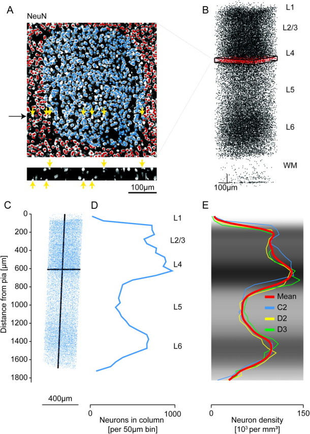
Number and distribution of NeuN-positive cell bodies. (A) Overlay of a maximum intensity NeuN immunofluorescence image with markers that were manually placed at the presumptive midpoints of NeuN-positive cell bodies (blue markers were located within the C2 barrel outline). Yellow arrows indicate examples of somata that were located at the edge of a slice and were contained to less than half in that slice (see reslice in the bottom panel; black arrow indicates reslice location); these neurons were counted in the adjacent slice; for estimates of the measurement error introduced by this counting procedure, see Materials and Methods and Discussion. (B) 29 159 markers identified as NeuN-positive somata in the region of interest comprising the C2 barrel column. Red: slice shown in (A). (C) 18 597 manually placed markers indicating NeuN-positive cell bodies within the C2 barrel column, which was defined by extrapolation of the barrel outline in L4 (see Fig. 1) along the vertical column axis (which was assumed to be perpendicular to the pial surface). (D) 1D profile of marker density projected onto the vertical column axis. (E) 1D profiles of NeuN density along the respective vertical column axis for the C2, D2, and D3 columns and the mean profile. Gray scale indicates mean NeuN density. Profiles were scaled to the length of a “standard” TC projection column (1840 μm, see Wimmer et al. 2010 and Results). The indicated layers represent approximate layer boundaries; for a quantitative definition of layer borders, see Figure 3, Table 2, and Results.
Number of Cells in a Column: Analysis of Tangential Serial Sections
After alignment and definition of the column circumference, we analyzed consecutive tangential sections (50 μm thickness) by marking each cell body as illustrated in Figure 2A. A marker was placed only if the maximum soma diameter was contained in the slice (for details of neuron counting, see Materials and Methods). We first manually labeled all cells in a rectangular region of interest surrounding the presumptive column outline (458 × 473 μm2 size, 40 sections for the C2 column, Fig. 2A,B). Then, the column outline as delineated in L4 was extrapolated to all layers along the presumptive column axis (Fig. 2C). The C2 column had a cross-sectional area of 135 922 μm2 and a height of 1711 μm, thus a column volume of 0.233 mm3. The total number of NeuN-positive somata in the thus-defined column was 18 597 (79 952 neurons per cubic millimeter, Table 1). NeuN-positive somata in the D2 column were counted similarly. For the D3 column, we used an automated soma counting method, which was calibrated to the manual counts of the C2 and D2 columns (see Oberlaender et al. 2009, Materials and Methods, and Supplementary Fig. 1). Together, this analysis yielded an average of 19 109 ± 444 neurons per column (Table 1). We also normalized the neuron number per column to the volume of the standard TC projection column as defined before (height 1840 μm, cross-sectional area 121 000 μm2, see Wimmer et al. 2010). Because all 3 columns evaluated here had slightly larger volumes than the presumed “standard column” (Table 2), the estimated number of neurons in a standard column was 17 560 ± 399 (i.e., 8% less than for the average counts, see Tables 1 and 2).
Table 1.
Neuron counts and neuron density for the C2, D2 and D3 barrel columns and the surrounding septa
| NeuN count |
NeuN density (103/mm3) |
NeuN count standard column |
||||||||||
| C2 | D2 | D3 | Mean ± SD | C2 | D2 | D3 | Mean ± SD | C2 | D2 | D3 | Mean ± SD | |
| L1 | 72 | 52 | 65 | 63 ± 10 | 9.6 | 4.9 | 5.2 | 6.6 ± 2.7 | 69 | 46 | 60 | 58 ± 12 |
| L2 | 2619 | 1897 | 1601 | 2039 ± 524 | 99.2 | 81.8 | 78.3 | 86.4 ± 11.2 | 2507 | 1674 | 1471 | 1884 ± 549 |
| L3 | 2727 | 4001 | 4478 | 3735 ± 905 | 107.7 | 94.8 | 102.3 | 101.6 ± 6.5 | 2610 | 3530 | 4115 | 3418 ± 758 |
| L4 | 4465 | 4877 | 3999 | 4447 ± 439 | 125.0 | 117.1 | 129.6 | 123.9 ± 6.3 | 4274 | 4303 | 3675 | 4084 ± 355 |
| L5A | 2011 | 1517 | 1684 | 1737 ± 251 | 54.0 | 50.5 | 58.8 | 54.4 ± 4.1 | 1925 | 1339 | 1547 | 1604 ± 297 |
| L5B | 2139 | 2231 | 2336 | 2235 ± 99 | 57.7 | 57.7 | 64.2 | 59.8 ± 3.8 | 2047 | 1969 | 2147 | 2054 ± 89 |
| L6A | 3687 | 3691 | 3980 | 3786 ± 168 | 91.9 | 91.7 | 93.3 | 92.3 ± 0.9 | 3529 | 3257 | 3657 | 3481 ± 204 |
| L6B | 877 | 1113 | 1208 | 1066 ± 170 | 37.7 | 43.3 | 44.8 | 42 ± 3.8 | 839 | 982 | 1110 | 977 ± 135 |
| L1-L6B | 18 597 | 19 379 | 19 351 | 19 109 ± 444 | 80.0 | 76.8 | 79.9 | 78.9 ± 1.8 | 17 801 | 17 099 | 17 781 | 17 560 ± 399 |
| Septuma | 8067a | 70.9a | ||||||||||
Notes: Neuron counts are based on exhaustive manual and automated counts of the complete volumes containing these columns. Standard column refers to a standardized TC projection column (Wimmer et al. 2010) of height 1840 μm and cross-sectional area 121 000 μm2. The height and area measurements for each column and layer are reported in Table 2.
Only a fraction of the septum surrounding the C2 column was evaluated (see Fig. 2).
Table 2.
Geometrical measurements for the C2, D2, and D3 barrel columns
| Height (μm) |
Area (103 μm2) |
Volume (mm3) |
||||||||||
| C2 | D2 | D3 | Mean ± SD | C2 | D2 | D3 | Mean ± SD | C2 | D2 | D3 | Mean ± SD | |
| L1 | 55 | 75 | 95 | 75 ± 20 | 0.007 | 0.011 | 0.013 | 0.01 ± 0.003 | ||||
| L2 | 194.2 | 163.9 | 154.5 | 171 ± 21 | 0.026 | 0.023 | 0.020 | 0.023 ± 0.003 | ||||
| L3 | 186.2 | 298 | 330.5 | 272 ± 76 | 0.025 | 0.042 | 0.044 | 0.037 ± 0.01 | ||||
| L4 | 262.7 | 294.3 | 233.1 | 263 ± 31 | 0.036 | 0.042 | 0.031 | 0.036 ± 0.005 | ||||
| L5A | 273.9 | 212.1 | 216.3 | 234 ± 35 | 0.037 | 0.030 | 0.029 | 0.032 ± 0.005 | ||||
| L5B | 273 | 273.2 | 274.7 | 274 ± 1 | 0.037 | 0.039 | 0.036 | 0.037 ± 0.001 | ||||
| L6A | 295 | 284.4 | 321.9 | 300 ± 19 | 0.040 | 0.040 | 0.043 | 0.041 ± 0.001 | ||||
| L6B | 171.2 | 181.4 | 203.4 | 185 ± 16 | 0.023 | 0.026 | 0.027 | 0.025 ± 0.002 | ||||
| L1-L6B | 1711 | 1782 | 1829 | 1774 ± 59 | 135.9 | 141.6 | 132.4 | 136.6 ± 4.6 | 0.233 | 0.252 | 0.242 | 0.242 ± 0.01 |
| Septuma | 0.113a | |||||||||||
Notes: Layer heights were determined by fits to the neuron density profiles (see Results and Materials and Methods).
Only a fraction of the septum surrounding the C2 column was evaluated (see Fig. 2).
Distribution of Neurons Along the Vertical Column Axis
We then computed the neuron density profile along the vertical column axis (shown in Fig. 2D for the C2 column). Next, we computed the density profiles for the C2, D2, and D3 columns, each normalized to the presumed standard column height of 1840 μm, and computed the mean neuron density profile (Fig. 2E). The mean neuron density had peaks in L4 (132 741 per cubic millimeter), upper L2/3 (104 664 per cubic millimeter), and upper L6 (98 282 per cubic millimeter) and minima in L1 (1855 per cubic millimeter) and L5 (49 598 per cubic millimeter).
To obtain the number of neurons per cortical layer in the column, we then used the neuron density profile for each of the columns to define layer borders along the vertical column axis. Layer borders were defined using Gaussian fits to the peaks of the profile (exemplified for the lower L4 border of the C2 column in Fig. 3A). The fitted layer border matched well with the apparent density drop in the anti-NeuN maximum intensity projection image (Fig. 3A, right panel). A border between L5A and L5B could not be defined based on the density of NeuN-positive somata (Fig. 3A, left panel). However, both the POm projection (Fig. 3B, right panel; profiles as in Meyer et al. 2010) and the GAD67 immunofluorescence images indicated a clear subdivision of layer 5. We used this subdivision to approximate the L5A-to-L5B border.
The ensuing layer heights are reported in Table 2, together with the normalized layer heights for a standardized projection column of height 1840 μm and a cross-sectional area of 121 000 μm2.
Number of Neurons Per Layer and Type in a Cortical Column
The delineation of layer borders then allowed the counting of neurons in each of the layers of a cortical column. We found that most neurons in a column are located in layer 4 (4447, see Table 1), followed by layer 6A (3786) and layer 3 (3735). Assuming an average fraction of non-excitatory (mostly GABAergic) interneurons (INs) of ∼15% (Lin et al. 1985; Beaulieu 1993), it follows that a cortical column contains the following number of excitatory neurons: 4908 in L2/3, 3780 in L4, 1477 in L5A (containing mostly “slender-tufted” pyramidal neurons), 1900 in L5B (containing mostly “thick-tufted” pyramidal neurons), and 4124 in L6.
The density-based layer borders do not necessarily correlate with the vertical distribution of neuron types. We therefore also estimated the number of neurons per neuron type (at the example of the D2 column) using layer borders derived from the recording depths of identified neurons (inset in Fig. 4A; layer borders were estimated as the average depth of the uppermost and deepest neuron of 2 neighboring layers, respectively). This yielded 6489 neurons in the supragranular layers, 4816 neurons in L4 (4094 spiny L4 neurons when corrected for INs), 1194 neurons in L5A (1015 slender-tufted pyramidal neurons), 1528 neurons in L5B (1299 thick-tufted pyramidal neurons), and 5352 neurons in L6. The underlying layer borders were (for a standard projection column) 586 μm (L3 pyramidal neuron to L4 spiny neuron), 919 μm (L4 spiny neuron to L5 slender-tufted pyramidal neuron), 1104 μm (L5 slender-tufted to L5 thick-tufted pyramidal neuron), and 1308 μm (L5 thick-tufted to L6 pyramidal neuron).
Figure 4.

Estimation of the number of action potentials emitted from a cortical column in response to a sensory stimulus. (A) Average number of APs per neuron type elicited by stimulation of the principal whisker within a 50 ms and 100 ms post-stimulus time window, respectively. Inset: Number of evoked APs per neuron in dependence of soma depth from the pia for the 100 ms time window (different colors illustrate different neuron types as determined by their dendritic morphology). Data from de Kock et al. (2007). (B) Number of excitatory neurons in a cortical column per type (Fig. 3A and Table 1). (C) Estimated number of APs evoked in a cortical column in response to stimulation of the principal whisker. Note that the majority of APs are emitted by spiny L4 neurons (35% within 50 ms, 34% within 100 ms time window) and thick-tufted L5 pyramidal neurons (28% in both time windows). For the number of spontaneous and the total number of APs within these time windows, see Table 3.
Neuron Density in the Septa Between Columns
We also measured the neuron density in the part of the septum-related cortex immediately surrounding the C2 column, which was part of the region of interest chosen for manual counting (see red markers in Fig. 2A). Neuron density was markedly lower in the septum-related cortex than within a column (71 000 vs. 80 000 per cubic millimeter, cf. Table 1).
Estimation of the Action Potential Output of a Single Cortical Column
The measurement of the number of neurons along the vertical column axis then provided a more precise quantification of the AP budget of a single cortical column in response to deflection of the principal whisker (for a first estimate, see de Kock et al. 2007). Figure 4A shows the recorded average number of APs in response to the stimulus in dependence of the neuron type and in dependence of the distance of the approximate soma location from the pia (inset in Fig. 4A, sorted by the cell type that was determined by the respective dendritic morphology). The average number of APs per neuron type was then multiplied by the estimated number of excitatory neurons per type (i.e., by the number of neurons per layer) in a column (Fig. 4B and Table 3). Figure 4C shows the resulting estimates of the number of APs evoked in excitatory neurons within a 50 and 100 ms time window after the stimulus, respectively. In the average column, most APs were evoked in the population of neurons in L4 (∼1500 APs evoked within 100 ms) and L5B (∼1200 APs evoked within 100 ms), and the sparsest AP output was from neurons in L5A (∼225 APs evoked within 100 ms). The estimated total number of APs generated by excitatory neurons within the home column was ∼3160 (50 ms post-stimulus) and ∼4440 (100 ms post-stimulus).
Table 3.
Estimates for the AP output of a cortical column in response to a stimulation of the principal whisker
| APs/neuron |
Number of excitatory cells | APs/column |
|||||||||||
| 50 ms post-stimulus |
100 ms post-stimulus |
50 ms post-stimulus |
100 ms post-stimulus |
||||||||||
| Spontaneous | Evoked | Total | Spontaneous | Evoked | Total | Spontaneous | Evoked | Total | Spontaneous | Evoked | Total | ||
| L2/3 | 0.02 | 0.07 | 0.08 | 0.03 | 0.10 | 0.13 | 4908 | 78 | 329 | 407 | 155 | 504 | 660 |
| L4 | 0.03 | 0.29 | 0.32 | 0.06 | 0.40 | 0.45 | 3780 | 107 | 1102 | 1208 | 214 | 1502 | 1715 |
| L5A (slender-tufted) | 0.05 | 0.03 | 0.09 | 0.11 | 0.15 | 0.26 | 1477 | 80 | 46 | 126 | 160 | 223 | 383 |
| L5B (thick-tufted) | 0.18 | 0.47 | 0.65 | 0.36 | 0.64 | 1.01 | 1900 | 347 | 896 | 1242 | 693 | 1225 | 1918 |
| L6(A) | 0.02 | 0.24 | 0.27 | 0.05 | 0.31 | 0.35 | 3218 | 75 | 783 | 858 | 150 | 987 | 1137 |
| L2-L6A | 15 283 | 686 | 3155 | 3841 | 1372 | 4441 | 5813 | ||||||
Notes: Number of APs per neuron generated in each of the excitatory cell types by stimulation of the principal whisker within the 50- and 100-ms post-stimulus interval from de Kock et al. (2007). Number of excitatory cells is estimated from the NeuN counts (see Table 1), corrected for an overall ratio of GABAergic INs of 15%.
Discussion
We measured the absolute number of neurons in 3 columns (C2, D2, and D3) in barrel cortex of a P27 rat. The number of neurons in a column is required for precise quantitative models of cortical function (Helmstaedter et al. 2007), for predictions about, for example, the AP budget of a column (de Kock et al. 2007), and for the quantification of TC innervation domains for the different types of excitatory neurons (the subsequent article, Meyer et al. 2010).
Comparison With Previous Results
Previous work has provided estimates of cell numbers and densities in different areas of the mammalian cortex using sampling-based density measurements (disector method: Sterio 1984; Beaulieu et al. 1992; Beaulieu 1993; Keller and Carlson 1999). Although the expected error of such measurements (based on the sampling statistics) is low (5–10%), the results from different studies disagreed widely, covering a range of almost a factor 2 (48 000 per cubic millimeter, Beaulieu 1993; 77 000 per cubic millimeter, Keller and Carlson 1999, for rat primary somatosensory cortex; similar disagreements can be found for primary visual cortex). Also, such measurements did only sparsely sample the different layers or septa versus columns. It was therefore not possible to derive numbers at the precision that is required for mechanistic modeling of whole-column or whole-layer circuits. The neuron density reported here (78 900 ± 1800 per cubic millimeter) agrees with the numbers reported by Keller and Carlson (1999).
Thick-tufted pyramidal cells in L5B have been reported to form “bundles” of apical dendrites (Fleischhauer et al. 1972; Peters and Walsh 1972; Krieger et al. 2007). The number of such bundles per column is approximately 150 (distance between bundles: ∼30 μm; Peters and Walsh 1972), with ∼7 apical dendrites per bundle, thus ∼1000 L5B pyramidal neurons forming bundles. This is a lower estimate for the number of excitatory neurons in L5B. Comparison with the number reported here (1300–1900, see above) suggests that only a fraction of the neurons in L5B contribute to the formation of apical dendrite bundles.
A recent study reports counts of neuronal cell bodies in mouse using the nuclear marker DAPI in 1400 μm-thick sections (Tsai et al. 2009). As expected for this section thickness, staining for NeuN is however reported to be too weak for consistent counting based on NeuN, only. We have used thin (50 μm) sections which provide rather homogeneous depth penetration of the NeuN-antibody and readily allow the identification of neuronal somata (Fig. 1D).
Shrinkage and Cutting Artifacts
The measurement of cell density is critically dependent on the definition of the volume within which the neuron counting was made. Therefore, shrinkage artifacts strongly affect the estimation of cell densities. The exhaustive analysis of one entire volume of interest, however, is not dependent on this uncertainty in the density measurement. Therefore, the total numbers of neurons in the whole column and in the cortical layers did not have to be corrected for shrinkage due to fixation and embedding artifacts.
The neuron density measurement (only provided for comparison with previous studies) was however sensitive to shrinkage artifacts. Given the accuracy of the slicer we used, slice thickness was assumed to be 50 μm regardless of the measured optical thickness of maximum intensity projections of confocal images of the slices. We found a thickness reduction (measured by optical slice thickness) of ∼10%, which was attributed to squeezing and shrinkage artifacts occurring during post-slicing processing of the slices. Shrinkage occurring during perfusion fixation was not quantified. Cutting of cell bodies at the slice border was an additional source of error; we controlled for an overestimation of neuron numbers due to this effect, estimating the resulting error to contribute only a slight overestimation (∼3%) of the neuron numbers (see Materials and Methods).
Precision of Layer Border Definitions
We used the neuron density profiles measured along the vertical column axis to define the borders between cortical layers. This definition was evident for the borders between the granular and infragranular layers due to the marked differences in cell densities at these transitions. However, the borders between most other layers are not as sharp as that between L4 and L5. Lack of sharp cytoarchitectonic borders causes a blur in the estimated number of cells in L2/3 and L4. In L4, a significant proportion of cells are star pyramidal cells (as defined by the shape of their dendritic arbors with a vertically oriented apical dendrite). The star pyramidal cells could be part of either L4 or L3 (Feldmeyer et al. 1999), the only morphological difference being the presence of an apical tuft in L3 pyramidal neurons. We used fits to the cell density profiles to delineate L4 from L2/3, which does not account for cell morphology.
Similarly, the distinction between L5A and L5B could not be justified based on the cell density profiles (Fig. 3A). Yet, the VPM projection pattern, the anti-GAD67 immunofluorescence, and even the native slice observed in brightfield illumination clearly show a sharp boundary within L5 (Fig. 1A,B). It can be speculated whether this delineation is due to other histological differences (e.g., axon density) or differences in IN density.
Estimate of the Fraction of GABAergic INs
For computing the number of excitatory neurons in the column, we have used a rough average estimate of the fraction of GABAergic INs of 15%. This corresponds to the numbers reported by Lin et al. (1985) and Beaulieu (1993) and roughly agrees with our own measurements (H.S.M., B.S., M.H., unpublished data). The effects of differences in IN ratio for different layers of the cortex on the quantitative predictions made here and in the subsequent manuscript (Meyer et al. 2010) are negligible compared with the effects of the uncertainty of geometrical measurements (see the subsequent article for an in-depth discussion of the magnitude of these errors).
Action Potential Counts
Using the average action potential responses of different cell types defined by their somatic and dendritic morphology (de Kock et al. 2007), the average representation of whisker deflection by action potentials in a cortical column can be estimated by simple multiplication with the number of excitatory neurons per layer (Fig. 4). The resulting estimate for the AP budget after whisker deflection depends thus on the precision of the estimated number of neurons. Previous estimates using the layer densities as reported in Beaulieu (1993) are now revised using the neuron numbers obtained in the present study. The estimated AP budget of a cortical column in response to a principal whisker deflection is 3155 and 4441 for the 50 and 100 ms post-stimulus interval, respectively (Table 3). Previous estimates that had to rely on available cell density measurements (Beaulieu 1993), only, had concluded ∼2400 APs to be evoked within the 100-ms post-stimulus interval (using the per-neuron AP rates reported in de Kock et al. (2007), which were also used in the present study). Note that these numbers summarize the “evoked” AP budget of a column, that is, those APs that are generated in addition to the spontaneous APs. Spontaneous APs in a cortical column are estimated to sum to 686 and 1372 in the 50- and 100-ms post-stimulus interval, respectively. Due to the lack of AP response data, L1 and L6B were not included in the present estimation.
These estimates of average AP output are likely to change if the response variability and the prevalence of the different cell types within a given layer can be accounted for. Here, we assumed that the measured cell types are representative for a particular layer that was defined on the basis of changes in neuron density. A limitation of our estimation is that the actual correspondence of neuron density–based layer borders (e.g., between L2/3 and L4) and the soma depth ranges of different morphological neuron types (e.g., of L3 pyramidal neurons and L4 star pyramidal neurons) remains unclear. The population responses of L4 and L2/3 estimated in this study could therefore vary depending on the actual number of neurons per type in a column. Using layer borders from in vivo recording depths of identified neurons to estimate the number of neurons per type yielded different population AP responses for neurons in L5 in the 100 ms interval (range: 837 vs. 1225 for L5 thick-tufted pyramidal neurons and 154 vs. 223 for slender-tufted pyramidal neurons). In L5, however, there may be no clear laminar separation between L5A and L5B containing slender- and thick-tufted cells at all (as indicated by the significant overlap of the 2 populations based on recording depth, see inset in Fig. 4A). This means that presumably not all excitatory L5A cells are thin tufted and not all L5B cells are thick tufted (Schubert et al. 2001, 2006; de Kock et al. 2007). Whether this apparent mismatch between the cell type definition based on soma location and cell morphology is due to variability in the depth measurements in in vivo recordings or represents an actual overlap of slender-tufted and thick-tufted pyramidal neuron somata in L5 is an unresolved issue. If there is cell type overlap, knowledge of the relative abundance of different neuron types in the cytoarchitectonic layers is thus required for a more precise estimation of type-specific population AP responses. Finally, the varying fraction of inhibitory cells between layers was not taken into account.
Relationship to Ontogenetic Columns
The concept of “cortical columns” has been applied to a variety of vertically organized assemblies of neurons in the neocortex based on functional (Mountcastle 1957, 1997; Hubel and Wiesel 1968), anatomical (Hubel and Wiesel 1969; Herkenham 1980; Koralek et al. 1988; Jones 2000; Rockland and Ichinohe 2004), and developmental (Rakic 1976, 1988) data. The concept of cortical columns has also been contested based on this apparent ambiguity in definition (Horton and Adams 2005; Douglas and Martin 2007). From the perspective of developmental studies, the finding of vertically oriented clonally related neurons has inspired the concept of ontogenetic columns, which (in the primate) constitute ensembles of on the order of 102 neurons each (Rakic 1988). As suggested by Rakic (1988), the assembly of functional cortical columns could then correspond to a lateral combination of such ontogenetic columns. This lateral integration of neurons into functional units could be governed both by local factors (which can be specifically disrupted; Torii et al. 2009) and by (external) sensory input. Following these notions, our sole criterion for defining a cortical column, that is, the dimensions of TC axonal projections, would represent such an external cue for assembling ontogenetic columns into functional cortical columns. In a rough estimate, the column size we report (∼19 000 neurons per column) may correspond to ∼190 ontogenetic columns. The detailed synaptic connectivity within a functional cortical column could be specific to these underlying ontogenetic cell lineages (Yu et al. 2009). Such clonally related groups of neurons however do not seem to correspond to such groups of pyramidal cells whose apical dendrites bundle as reported for L5 (Rockland and Ichinohe 2004; Krieger et al. 2007). It remains to be investigated to which degree the number of neurons in functional columns (as defined by common sensory input) in other cortical areas and species differ from the number of neurons in a cortical column from rat vibrissal cortex as defined here on the basis of TC axonal projections.
Outlook
We have provided the number of neurons per layer in a cortical column that was defined by the approximate TC projection volume. The variability of neuron numbers within cortical columns both between animals and within the barrel field is still unknown. Our data indicate that at least the latter may be rather low (less than 10%, see Table 1). Another future issue is to define more clearly how many cells of a particular cell type (as defined by the geometry of its dendrites or its axonal arbor projection targets) are contributing to the number of cells in a particular layer. Apart from the division in excitatory and inhibitory cells, it is expected that further subdivisions will be found between different “soma–dendritic types” of cells in a layer as it is exemplified by thin- and thick-tufted pyramidal neurons in L5. Using specific genetic markers for individual dendritic cell types that are now available (Heintz 2004) is probably one way how estimates of the fraction of various subtypes in a column and within a particular layer may be obtained (Groh et al. 2009).
The results of this study are essential for a quantitative description of the amount of TC input to a cortical column, as reported in the subsequent article (Meyer et al. 2010).
Supplementary Material
Supplementary material can be found at: http://www.cercor.oxfordjournals.org/
Funding
Max Planck Society.
Supplementary Material
Acknowledgments
We thank Marlies Kaiser and Ellen Stier for histology; Rolf Rödel and Karl Schmidt for technical assistance; Daniel Schwarz, Anna Meier, Zeynep Aydin, Christina Ernst, Jana Hechler, and Betty Pickard for neuron counting; and Guenter Giese for providing an excellent imaging facility. Conflict of Interest: None declared.
Author contributions: Conceived and designed the experiments: H.S.M., V.C.W., B.S., and M.H. (neuron counts and virus injections); C.P.J.d.K. and B.S. (AP measurements). Contributed adeno-associated virus: V.C.W. Performed the experiments: H.S.M. (neuron counts and virus injections) and C.P.J.d.K. (AP measurements). Analyzed the data: H.S.M., M.O., B.S., and M.H. Wrote the paper: H.S.M. and M.H.
References
- Beaulieu C. Numerical data on neocortical neurons in adult rat, with special reference to the GABA population. Brain Res. 1993;609:284–292. doi: 10.1016/0006-8993(93)90884-p. [DOI] [PubMed] [Google Scholar]
- Beaulieu C, Kisvarday Z, Somogyi P, Cynader M, Cowey A. Quantitative distribution of GABA-immunopositive and -immunonegative neurons and synapses in the monkey striate cortex (area 17) Cereb Cortex. 1992;2:295–309. doi: 10.1093/cercor/2.4.295. [DOI] [PubMed] [Google Scholar]
- de Kock CP, Bruno RM, Spors H, Sakmann B. Layer- and cell-type-specific suprathreshold stimulus representation in rat primary somatosensory cortex. J Physiol. 2007;581:139–154. doi: 10.1113/jphysiol.2006.124321. [DOI] [PMC free article] [PubMed] [Google Scholar]
- Douglas RJ, Martin KA. Mapping the matrix: the ways of neocortex. Neuron. 2007;56:226–238. doi: 10.1016/j.neuron.2007.10.017. [DOI] [PubMed] [Google Scholar]
- Feldmeyer D, Egger V, Lubke J, Sakmann B. Reliable synaptic connections between pairs of excitatory layer 4 neurones within a single ‘barrel’ of developing rat somatosensory cortex. J Physiol. 1999;521(Pt 1):169–190. doi: 10.1111/j.1469-7793.1999.00169.x. [DOI] [PMC free article] [PubMed] [Google Scholar]
- Fleischhauer K, Petsche H, Wittkowski W. Vertical bundles of dendrites in the neocortex. Z Anat Entwicklungsgesch. 1972;136:213–223. doi: 10.1007/BF00519179. [DOI] [PubMed] [Google Scholar]
- Groh A, Meyer HS, Schmidt EF, Heintz N, Sakmann B, Krieger P. Cell-type specific properties of pyramidal neurons in neocortex underlying a layout that is modifiable depending on the cortical area. Cereb Cortex. 2009;20(4):826–836. doi: 10.1093/cercor/bhp152. [DOI] [PubMed] [Google Scholar]
- Heintz N. Gene expression nervous system atlas (GENSAT) Nat Neurosci. 2004;7:483. doi: 10.1038/nn0504-483. [DOI] [PubMed] [Google Scholar]
- Helmstaedter M, de Kock CP, Feldmeyer D, Bruno RM, Sakmann B. Reconstruction of an average cortical column in silico. Brain Res Rev. 2007;55:193–203. doi: 10.1016/j.brainresrev.2007.07.011. [DOI] [PubMed] [Google Scholar]
- Herkenham M. Laminar organization of thalamic projections to the rat neocortex. Science. 1980;207:532–535. doi: 10.1126/science.7352263. [DOI] [PubMed] [Google Scholar]
- Horton JC, Adams DL. The cortical column: a structure without a function. Philos Trans R Soc Lond B Biol Sci. 2005;360:837–862. doi: 10.1098/rstb.2005.1623. [DOI] [PMC free article] [PubMed] [Google Scholar]
- Hubel DH, Wiesel TN. Receptive fields and functional architecture of monkey striate cortex. J Physiol. 1968;195:215–243. doi: 10.1113/jphysiol.1968.sp008455. [DOI] [PMC free article] [PubMed] [Google Scholar]
- Hubel DH, Wiesel TN. Anatomical demonstration of columns in the monkey striate cortex. Nature. 1969;221:747–750. doi: 10.1038/221747a0. [DOI] [PubMed] [Google Scholar]
- Jones EG. Microcolumns in the cerebral cortex. Proc Natl Acad Sci U S A. 2000;97:5019–5021. doi: 10.1073/pnas.97.10.5019. [DOI] [PMC free article] [PubMed] [Google Scholar]
- Julien JF, Samama P, Mallet J. Rat brain glutamic acid decarboxylase sequence deduced from a cloned cDNA. J Neurochem. 1990;54:703–705. doi: 10.1111/j.1471-4159.1990.tb01928.x. [DOI] [PubMed] [Google Scholar]
- Kaufman DL, McGinnis JF, Krieger NR, Tobin AJ. Brain glutamate decarboxylase cloned in lambda gt-11: fusion protein produces gamma-aminobutyric acid. Science. 1986;232:1138–1140. doi: 10.1126/science.3518061. [DOI] [PMC free article] [PubMed] [Google Scholar]
- Keller A, Carlson GC. Neonatal whisker clipping alters intracortical, but not thalamocortical projections, in rat barrel cortex. J Comp Neurol. 1999;412:83–94. doi: 10.1002/(sici)1096-9861(19990913)412:1<83::aid-cne6>3.0.co;2-7. [DOI] [PubMed] [Google Scholar]
- Kobayashi Y, Kaufman DL, Tobin AJ. Glutamic acid decarboxylase cDNA: nucleotide sequence encoding an enzymatically active fusion protein. J Neurosci. 1987;7:2768–2772. doi: 10.1523/JNEUROSCI.07-09-02768.1987. [DOI] [PMC free article] [PubMed] [Google Scholar]
- Koralek KA, Jensen KF, Killackey HP. Evidence for two complementary patterns of thalamic input to the rat somatosensory cortex. Brain Res. 1988;463:346–351. doi: 10.1016/0006-8993(88)90408-8. [DOI] [PubMed] [Google Scholar]
- Krieger P, Kuner T, Sakmann B. Synaptic connections between layer 5B pyramidal neurons in mouse somatosensory cortex are independent of apical dendrite bundling. J Neurosci. 2007;27:11473–11482. doi: 10.1523/JNEUROSCI.1182-07.2007. [DOI] [PMC free article] [PubMed] [Google Scholar]
- Lin CS, Lu SM, Schmechel DE. Glutamic acid decarboxylase immunoreactivity in layer IV of barrel cortex of rat and mouse. J Neurosci. 1985;5:1934–1939. doi: 10.1523/JNEUROSCI.05-07-01934.1985. [DOI] [PMC free article] [PubMed] [Google Scholar]
- Meyer HS, Wimmer VC, Hemberger M, Bruno RM, de Kock CP, Frick A, Sakmann B, Helmstaedter M. Cell-type specific thalamic innervation in a column of rat vibrissal cortex. Cereb Cortex. 2010 doi: 10.1093/cercor/bhq069. doi: 10.1093/cercor/bhq069. [DOI] [PMC free article] [PubMed] [Google Scholar]
- Mountcastle VB. Modality and topographic properties of single neurons of cat's somatic sensory cortex. J Neurophysiol. 1957;20:408–434. doi: 10.1152/jn.1957.20.4.408. [DOI] [PubMed] [Google Scholar]
- Mountcastle VB. The columnar organization of the neocortex. Brain. 1997;120(Pt 4):701–722. doi: 10.1093/brain/120.4.701. [DOI] [PubMed] [Google Scholar]
- Mullen RJ, Buck CR, Smith AM. NeuN, a neuronal specific nuclear protein in vertebrates. Development. 1992;116:201–211. doi: 10.1242/dev.116.1.201. [DOI] [PubMed] [Google Scholar]
- Oberlaender M, Dercksen VJ, Egger R, Gensel M, Sakmann B, Hege HC. Automated three-dimensional detection and counting of neuron somata. J Neurosci Methods. 2009;180:147–160. doi: 10.1016/j.jneumeth.2009.03.008. [DOI] [PubMed] [Google Scholar]
- Peters A, Walsh TM. A study of the organization of apical dendrites in the somatic sensory cortex of the rat. J Comp Neurol. 1972;144:253–268. doi: 10.1002/cne.901440302. [DOI] [PubMed] [Google Scholar]
- Rakic P. Prenatal genesis of connections subserving ocular dominance in the rhesus monkey. Nature. 1976;261:467–471. doi: 10.1038/261467a0. [DOI] [PubMed] [Google Scholar]
- Rakic P. Specification of cerebral cortical areas. Science. 1988;241:170–176. doi: 10.1126/science.3291116. [DOI] [PubMed] [Google Scholar]
- Rockland KS, Ichinohe N. Some thoughts on cortical minicolumns. Exp Brain Res. 2004;158:265–277. doi: 10.1007/s00221-004-2024-9. [DOI] [PubMed] [Google Scholar]
- Schubert D, Kotter R, Luhmann HJ, Staiger JF. Morphology, electrophysiology and functional input connectivity of pyramidal neurons characterizes a genuine layer va in the primary somatosensory cortex. Cereb Cortex. 2006;16:223–236. doi: 10.1093/cercor/bhi100. [DOI] [PubMed] [Google Scholar]
- Schubert D, Staiger JF, Cho N, Kotter R, Zilles K, Luhmann HJ. Layer-specific intracolumnar and transcolumnar functional connectivity of layer V pyramidal cells in rat barrel cortex. J Neurosci. 2001;21:3580–3592. doi: 10.1523/JNEUROSCI.21-10-03580.2001. [DOI] [PMC free article] [PubMed] [Google Scholar]
- Sterio DC. The unbiased estimation of number and sizes of arbitrary particles using the disector. J Microsc. 1984;134:127–136. doi: 10.1111/j.1365-2818.1984.tb02501.x. [DOI] [PubMed] [Google Scholar]
- Torii M, Hashimoto-Torii K, Levitt P, Rakic P. Integration of neuronal clones in the radial cortical columns by EphA and ephrin-A signalling. Nature. 2009;461:524–528. doi: 10.1038/nature08362. [DOI] [PMC free article] [PubMed] [Google Scholar]
- Tsai PS, Kaufhold JP, Blinder P, Friedman B, Drew P, Karten HJ, Lyden PD, Kleinfeld D. Correlations of Neuronal and Microvascular Densities in Murine Cortex Revealed by Direct Counting and Colocalization of Nuclei and Vessels. J Neurosci. 2009;29:14553–14570. doi: 10.1523/JNEUROSCI.3287-09.2009. [DOI] [PMC free article] [PubMed] [Google Scholar]
- Wimmer VC, Bruno RM, de Kock CP, Kuner T, Sakmann B. Dimensions of a projection column and architecture of VPM- and POm-axons in rat vibrissal cortex. doi: 10.1093/cercor/bhq068. Cereb Cortex. doi: 10.1093/cercor/bhq068. [DOI] [PMC free article] [PubMed] [Google Scholar]
- Wimmer VC, Nevian T, Kuner T. Targeted in vivo expression of proteins in the calyx of Held. Pflugers Arch. 2004;449:319–333. doi: 10.1007/s00424-004-1327-9. [DOI] [PubMed] [Google Scholar]
- Yu YC, Bultje RS, Wang X, Shi SH. Specific synapses develop preferentially among sister excitatory neurons in the neocortex. Nature. 2009;458:501–504. doi: 10.1038/nature07722. [DOI] [PMC free article] [PubMed] [Google Scholar]
Associated Data
This section collects any data citations, data availability statements, or supplementary materials included in this article.