Combining Machine Learning and Homology-Based Approaches to Accurately Predict Subcellular Localization in Arabidopsis^,,,

Abstract

A complete map of the Arabidopsis (Arabidopsis thaliana) proteome is clearly a major goal for the plant research community in terms of determining the function and regulation of each encoded protein. Developing genome-wide prediction tools such as for localizing gene products at the subcellular level will substantially advance Arabidopsis gene annotation. To this end, we performed a comprehensive study in Arabidopsis and created an integrative support vector machine-based localization predictor called AtSubP (for Arabidopsis subcellular localization predictor) that is based on the combinatorial presence of diverse protein features, such as its amino acid composition, sequence-order effects, terminal information, Position-Specific Scoring Matrix, and similarity search-based Position-Specific Iterated-Basic Local Alignment Search Tool information. When used to predict seven subcellular compartments through a 5-fold cross-validation test, our hybrid-based best classifier achieved an overall sensitivity of 91% with high-confidence precision and Matthews correlation coefficient values of 90.9% and 0.89, respectively. Benchmarking AtSubP on two independent data sets, one from Swiss-Prot and another containing green fluorescent protein- and mass spectrometry-determined proteins, showed a significant improvement in the prediction accuracy of species-specific AtSubP over some widely used “general” tools such as TargetP, LOCtree, PA-SUB, MultiLoc, WoLF PSORT, Plant-PLoc, and our newly created All-Plant method. Cross-comparison of AtSubP on six nontrained eukaryotic organisms (rice [Oryza sativa], soybean [Glycine max], human [Homo sapiens], yeast [Saccharomyces cerevisiae], fruit fly [Drosophila melanogaster], and worm [Caenorhabditis elegans]) revealed inferior predictions. AtSubP significantly outperformed all the prediction tools being currently used for Arabidopsis proteome annotation and, therefore, may serve as a better complement for the plant research community. A supplemental Web site that hosts all the training/testing data sets and whole proteome predictions is available at http://bioinfo3.noble.org/AtSubP/.

Subcellular proteomics has gained tremendous attention of late, owing to the role played by organelles in carrying out defined cellular processes. Several experimental efforts have been made to catalog the complete subcellular proteomes of various organisms (Michaud and Snyder, 2002; Huh et al., 2003; Taylor et al., 2003; Andersen and Mann, 2006), with the aim being to improve our understanding of defined cellular processes at the organellar and cellular levels. Although such efforts have generated valuable information, cataloging all subcellular proteomes is far from complete, as experimental methods are expensive and more time consuming. Alternatively, computational prediction systems provide fast, economic (mostly free), automatic, and reasonably accurate assignment of subcellular location to a protein, especially for high-throughput analysis of large-scale genome sequences, ultimately giving the right direction to design cost-effective wet-lab experiments.

The existing bioinformatics localization predictors in the literature can be broadly grouped into three categories: (1) amino acid composition based; (2) N-terminal sorting signals based; and (3) homology based (e.g. those based on domain or motif co-occurrence). These methods have previously been reviewed in detail (Mott et al., 2002; Scott et al., 2004). However, in bioinformatics in general, and in subcellular localization prediction in particular, it is often debated whether predictions should be done over broad systematic groups such as all eukaryotes or all plants, or over narrower groups such as dicots, or even at the single-species level. On the one hand, species-specific features of sorting signals and amino acid composition could make the prediction better if trained on the particular species where it is going to be used; on the other hand, the smaller data set available for a single species could make the single-species predictor less accurate. How to strike the balance between these two concerns is an important question, which has received far too little attention until now. In this study, we have investigated this important question by conducting a systematic species-specific case study on predicting subcellular localization in Arabidopsis (Arabidopsis thaliana). Although some recent reviews/advances in the prediction of protein-targeting signals have stressed the need for “species-specific” prediction tools (Schneider and Fechner, 2004; Chou and Shen, 2007a), very few have been developed/reported in the literature. The PSLT method (Scott et al., 2004), a Bayesian framework that uses a combination of InterPro motifs, signaling peptides, and transmembrane domains, was developed for predicting genome-wide subcellular localization of human proteins. Two others, HSLpred (Garg et al., 2005) and Hum-PLoc (Chou and Shen, 2006), were also developed specifically for human proteins; another species-specific system, TBpred, was developed for Mycobacterium tuberculosis (Rashid et al., 2007). However, none of these methods have rigorously tested whether their species-specific methods were actually better than the “general” ones.

In plants, some widely used prediction tools are TargetP (Emanuelsson et al., 2000), LOCtree (Nair and Rost, 2005), PA-SUB (Lu et al., 2004), MultiLoc (Höglund et al., 2006), WoLF PSORT (updated version of PSORT II; Horton et al., 2007), and Plant-PLoc (Chou and Shen, 2007b), all having good accuracy (greater than 70%). A recent computational effort was made in developing a plant species-specific prediction system, RSLpred, for genome-wide subcellular localization annotations of rice (Oryza sativa) proteins (Kaundal and Raghava, 2009). However, although Arabidopsis was the first model plant that was completely sequenced back in the year 2000, there is still no efficient prediction method available for accurately annotating its proteome at the subcellular level. To date, we only know the subcellular localization of about 6,000 proteins that are experimentally proven (e.g. using GFP fusions, mass spectrometry [MS], or other approaches) out of the total 27,379 protein-coding genes as predicted by The Arabidopsis Information Resource (TAIR) release 9 (www.arabidopsis.org). To narrow this huge gap between the large number of predicted genes in the Arabidopsis genome and the limited experimental characterization of their corresponding proteins, a fully automatic and reliable prediction system for complete subcellular annotation of the Arabidopsis proteome would be very useful.

This article presents AtSubP (for Arabidopsis subcellular localization predictor), an integrative system that addresses the aforementioned issues and problems. In this study, we develop this species-specific predictor and rigorously compare its performance with some of the widely used general tools, including the one being currently used by TAIR (Rhee et al., 2003), and discuss if species-specific predictors are more suitable for individual proteome-wide annotations. AtSubP uses the combinatorial presence of diverse features of a protein sequence, such as its amino acid composition, residue order-based dipeptide composition, N- and C-terminal composition, similarity search-based Position-Specific Iterated (PSI)-BLAST information, and the Position-Specific Scoring Matrix (PSSM), as its evolutionary information in a statistically coherent manner. Under five major classification approaches, we devised 15 different possible techniques to develop 105 different classifiers for each of the seven subcellular compartments under study (chloroplast, cytoplasm, Golgi apparatus, mitochondrion, extracellular, nucleus, and plasma membrane). The performance of these models was systematically evaluated based on a 5-fold cross-validation test and two diverse independent tests: one from Swiss-Prot and the other containing MS/GFP-proven sequences as an experimental test data set from the SUBcellular location database for Arabidopsis (SUBA; http://suba.plantenergy.uwa.edu.au/) and the eukaryotic Subcellular Localization DataBase (eSLDB; http://gpcr.biocomp.unibo.it/esldb/). Our novel approach of combining some diverse protein features into a smart hybrid technique led to the best classifier that achieved an outstanding accuracy level of 91%, with a high-confidence precision and Matthews correlation coefficient (MCC) of 90.9% and 0.89, respectively. The similarity search-based PSI-BLAST module alone performed moderately, achieving an overall accuracy of 78%, suggesting the advantages of machine learning-based classifiers.

To expand on the application and data-mining aspects of the method, we cross-matched the AtSubP’s predictions with the available Swiss-Prot and TAIR annotations as well as compared its performance with some of the widely used general tools on both independent test sets. To explore the species-specific effects, a new All-Plant classifier was developed from a mixture of plant proteins using the same location definitions and encoding schemes as in AtSubP, and their performances were compared in an independent testing. As another benchmark, the performance of an Arabidopsis-specific classifier was cross-checked on six other eukaryotic organisms (rice [Oryza sativa], soybean [Glycine max], human [Homo sapiens], yeast [Saccharomyces cerevisiae], fruit fly [Drosophila melanogaster], and worm [Caenorhabditis elegans]). The basic purpose of all these diverse tests was to explore the advantages of developing a species-specific predictor(s), if any. To further test this hypothesis, we also analyzed the variation in amino acid composition across various eukaryotic organisms and compared with Arabidopsis, both at the sequence level and in the signal peptide-containing regions.

Finally, AtSubP was used to annotate all 27,379 Arabidopsis proteins contained in TAIR release 9; among them, 21,649 (79.1%) proteins were predicated with their localization information, 7,982 (29.2%) sequences being predicted with high confidence. A user-friendly Web server, available at http://bioinfo3.noble.org/AtSubP/, was also developed to host all the training/testing data sets, whole proteome annotations, and options for annotating the query sequences using five diverse prediction modules based on user selection of protein feature(s).

RESULTS

The prediction accuracy was assessed by two distinct approaches: a 5-fold cross-validation test and the independent data set tests. In order to achieve maximum accuracy, a total of 105 different classifiers corresponding to seven subcellular localizations from 15 different techniques (15 × 7 = 105) were attempted under five broad alternative encoding schemes followed (described in detail in “Materials and Methods”). In this article, we have presented and discussed only the best classifier results; individual results tables of all other classifiers and their supporting material can be found in the Supplemental Data. However, the performance comparison of overall sensitivities achieved by these 15 diverse techniques constructed on the basis of different features of a protein sequence is presented in Figure 1.

Figure 1.

Performance comparison of overall sensitivities achieved by PSI-BLAST and various SVM modules constructed on the basis of different features of a protein sequence. For detailed performance of each classifier, see individual tables in Supplemental Data.

Statistical Tests of the Best Classifier

In the 5-fold cross-validation test, of all the diverse approaches followed to attain maximum performance, the best overall sensitivity was achieved from a hybrid-based technique (H-IX) combining the simple amino acid composition (AA), PSSM-based evolutionary information, and terminal-based N-Center-C composition with the binary output of PSI-BLAST (Table I). To decide on the statistical significance of one classifier over the other, we systematically calculated the P values at the 0.05 level of significance between every two classifiers based on their overall sensitivities achieved in a 5-fold cross-validation test. The P values as presented in Supplemental Table S1 reveal that the H-IX combination, which achieved the highest accuracy, was significant over all the modules developed except for the H-VII combination. This means that the overall sensitivity achieved by H-VII was statistically at par with the overall sensitivity achieved by H-IX. However, we noted that H-IX revealed higher prediction accuracy by using less dimensional vector (488 D) as compared with the 508-D vector length in H-VII. Moreover, within the same 488-D input vectors, H-IX showed significant improvement over H-VIII when using PSSM-based information in H-IX instead of dipeptide composition as used in H-VIII (Supplemental Table S1). Therefore, we considered H-IX as the best classifier and used it in our further analysis as discussed below.

Table I. Performance of the best classifier of AtSubP based on different statistical measures of quality.

Best classifier is based on the AA+PSSM+N-Center-C+PSI-BLAST hybrid combination and best results using the RBF kernel (γ = 3, C = 2, j = 2).

Subcellular Location	No. of Sequences	Sensitivity	Precision	Specificity	MCC	Error Rate
		%	%	%		%
Chloroplast	601	85.9	88.4	97.4	0.84	4.8
Cytoplasm	220	75.9	81.5	98.7	0.77	2.8
Golgi apparatus	106	86.8	82.9	99.4	0.84	1.0
Mitochondria	391	84.1	86.8	98.2	0.83	3.5
Extracellular	452	97.6	95.0	99.2	0.96	1.1
Nucleus	1,197	96.7	95.3	97.2	0.94	3.0
Plasma membrane	247	89.1	85.9	98.8	0.86	2.0
Overall	3,214	91.0	90.9	97.9	0.89	3.0

This classifier achieved an overall prediction accuracy (sensitivity) of 91% with a high-confidence MCC of 0.89. Sensitivity and specificity are two competing but nonexclusive measures of quality useful for testing the performance of classification methods. The MCC provides a balanced measure between sensitivity and specificity for each class. An ideal classification method should have both sensitivity and specificity values close to 100%. Referring to Table I, our specificity rates were also almost near 100%. Even at the highest sensitivity level, the specificity rates were still above 97.2%. In other words, the worst case false-positive rate expected for any location would not be greater than 2.8%. This classifier also showed a high-confidence precision of more than 90%, also called as the positive predictive value, and a very low error rate (3.0%), which indicated a highly reliable and accurate classifier. The individual statistics obtained with this best classifier for each of the seven subcellular localizations (Table I) indicated that “nucleus” and “secreted” proteins achieved the highest prediction accuracies of more than 96% (i.e. these sequences might have some unique nuclear localization signals and signal peptides, respectively, as compared with the other proteins in the data set), and that is why they were better identifiable through the machine-learned classifiers. However, cytoplasm and mitochondria were comparatively the least performing categories among all, achieving low sensitivities (75.9% for cytoplasm and 84.1% for mitochondria). Mitochondrial proteins are the most difficult to predict, as also proven in some of the earlier studies (Peng and Rajapakse, 2005; Sarda et al., 2005). On the other hand, the low performance of cytoplasm as compared with other categories was probably because it is the default location for protein synthesis as well as the hub of cellular core metabolism; therefore, it is likely to have the most “shared” functional domains, thus negatively affecting the prediction performance. Individual tables showing the results of other classifiers developed in this study are provided in Supplemental Tables S7a to S20a.

Benchmarking on Independent Data Sets and Comparison with Other Prediction Programs

Independent testing is the better approach to test the accuracy of a classifier, as the sequences used in these data sets are never seen by the system during the training process. We created two independent data sets, one from the Swiss-Prot database and the other containing experimentally annotated sequences from SUBA/eSLDB databases (for details, see “Materials and Methods”). As shown in Table II, the overall prediction accuracy of AtSubP on independent testing set I was about 85.2% (i.e. 304 protein sequences were correctly predicted out of the total 357 sequences in this set). Similarly, 64 sequences were correctly predicted by AtSubP out of the total 84 protein sequences in the experimentally proven independent data set II, thereby achieving an overall accuracy of 76.2% (Table III).

Table II. Performance of AtSubP in comparison with other methods on independent data set I of Arabidopsis proteins from Swiss-Prot.

Subcellular Location	No. of Sequences	Our Method Percentage Accuracy	TargetP Percentage Accuracy	LOCtree Percentage Accuracy	PA-SUB Percentage Accuracy	MultiLoc Percentage Accuracy	Wolf PSORT Percentage Accuracy	Plant-PLoc Percentage Accuracy
Chloroplast	67	76.1 (51)a	70.2 (47)	47.8 (32)	53.7 (36)	52.2 (35)	68.7 (46)	37.3 (25)
Cytoplasm	24	79.2 (19)	–b	58.3 (14)	70.8 (17)	58.3 (14)	70.8 (17)	41.7 (10)
Golgi apparatus	12	58.3 (7)	–b	00.0 (0)	08.3 (1)	16.7 (2)	25.0 (3)	–b
Mitochondria	43	65.1 (28)	53.5 (23)	41.9 (18)	48.8 (21)	44.2 (19)	27.9 (12)	11.6 (5)
Extracellular	50	96.0 (48)	86.0 (43)	70.0 (35)	70.0 (35)	64.0 (32)	16.0 (8)	30.0 (15)
Nucleus	133	99.3 (132)	–b	75.9 (101)	74.4 (99)	73.7 (98)	79.0 (105)	56.4 (75)
Plasma membrane	28	67.9 (19)	–b	–b	10.7 (3)	17.9 (5)	28.6 (8)	35.7 (10)
Overall accuracy	357	85.2 (304/357)	70.3 (113/160)	60.8 (200/329)	59.4 (212/357)	57.4 (205/357)	55.7 (199/357)	40.6 (140/345)

^aValues in parentheses represent the number of correctly predicted sequences.

^bPrediction not available.

Table III. Performance of AtSubP in comparison with other methods on an experimentally proved independent data set II of Arabidopsis proteins from SUBA/eSLDB.

Subcellular Location	No. of Sequences	Our Method Percentage Accuracy	TargetP Percentage Accuracy	LOCtree Percentage Accuracy	PA-SUB Percentage Accuracy	MultiLoc Percentage Accuracy	Wolf PSORT Percentage Accuracy	Plant-PLoc Percentage Accuracy
Chloroplast	20	70.0 (14)a	50.0 (10)	60.0 (12)	30.0 (6)	45.0 (9)	45.0 (9)	65.0 (13)
Cytoplasm	1	100.0 (1)	–b	00.0 (0)	100.0 (1)	00.0 (0)	100.0 (1)	00.0 (0)
Golgi apparatus	1	100.0 (1)	–b	00.0 (0)	00.0 (0)	00.0 (0)	00.0 (0)	–b
Mitochondria	8	62.5 (5)	37.5 (3)	25.0 (2)	37.5 (3)	37.5 (3)	25.0 (2)	00.0 (0)
Extracellular	1	100.0 (1)	100.0 (1)	100.0 (1)	00.0 (0)	00.0 (0)	00.0 (0)	00.0 (0)
Nucleus	44	81.8 (36)	–b	45.5 (20)	50.0 (22)	54.6 (24)	45.5 (20)	27.3 (12)
Plasma membrane	9	66.7 (6)	–b	–b	33.3 (3)	22.2 (2)	33.3 (3)	33.3 (3)
Overall accuracy	84	76.2 (64/84)	48.3 (14/29)	46.7 (35/75)	41.7 (35/84)	45.2 (38/84)	41.7 (35/84)	33.7 (28/83)

^aValues in parentheses represent the number of correctly predicted sequences.

^bPrediction not available.

We further evaluated the performance of our species-specific approach (i.e. AtSubP) in comparison with some widely used general methods, as most of the research community relies on these tools for their subcellular annotations. For example, TAIR is currently using the TargetP system (Emanuelsson et al., 2000) for annotating the complete subcellular proteome of Arabidopsis (ftp://ftp.arabidopsis.org/home/tair/Proteins/Properties/TargetP_analysis.tair9). We compared not only TargetP but some other tools, such as LOCtree (Nair and Rost, 2005), PA-SUB (Lu et al., 2004), MultiLoc (Höglund et al., 2006), WoLF PSORT (Horton et al., 2007), and Plant-PLoc (Chou and Shen, 2007b), all of which originally reported good accuracy. However, a number of previous researchers (Emanuelsson, 2002; Heazlewood et al., 2004, 2005) found only 40% to 50% accuracy of the existing systems in their experimental data sets when testing the available tools for Arabidopsis annotation. They all had recommended developing new prediction systems in the future, especially for the target species, if enough training data are available. We also tested the performance of these prediction tools with our Arabidopsis-specific independent sets (I and II); the results are shown in Tables II and III. In both independent test sets, the best overall performance was achieved by TargetP (70.6% on set I and 48.3% on set II) followed by LOCtree (60.8% on set I and 46.7% on set II) among the compared tools. Although these accuracies were quite lower as compared with the performance of our AtSubP method (85.2% on set I and 76.2% on set II), TargetP still continues to perform well in spite of its being one of the oldest methods, followed by LOCtree, which provides more localization coverage as compared with TargetP. On the other hand, some of the latest developed tools, like WoLF PSORT and Plant-PLoc, performed badly over both of these independent sets. For example, WoLF PSORT correctly predicted with an overall accuracy of only 55.7% and 41.7% on sets I and II, respectively. Similarly, the recently developed Plant-PLoc also showed a low overall prediction accuracy (i.e. 40.6% on set I and 33.7% on set II). PA-SUB, which originally reported high accuracy, also showed average (59.4% on set I) to below average (41.7% on set II) overall accuracy in our Arabidopsis-specific independent test sets. The individual performance of each localization class in these prediction servers is given in Table II for set I and Table III for set II.

In the experimentally annotated test sequences (set II), we observed a substantially improved performance of AtSubP (greater than 76% accuracy) over the general methods, which performed poorly (all less than 50% accuracy). Even TargetP showed inferior results on this test set (only 48.3% accuracy) as compared with its performance on test set I (70.6% overall accuracy). Second, all these general methods revealed the same trend of performance on both the independent data sets (i.e. TargetP showed the highest accuracy, followed by LOCtree, PA-SUB, MultiLoc, WoLF PSORT, and Plant-PLoc). It is worth mentioning here that TargetP still continues to predict with fairly good accuracy. Probably, that is why this tool is being used widely by the plant research community (e.g. TAIR uses it for annotating the Arabidopsis proteome). However, the accuracy of our method was significantly higher than TargetP on both these independent data sets (about 15% on test set I and 28% on experimentally annotated test set II). Another advantage of our system is that it provides subcellular predictions for seven classes as compared with only three (chloroplast, mitochondria, and extracellular) by TargetP. Therefore, keeping in view these two major advantages, we believe that AtSubP will act as a useful tool for better annotating the whole subcellular proteome of Arabidopsis.

Comparison with the Corresponding All-Plant Method

As each of the general methods mentioned above have been developed using different training data sets and following diverse classification techniques, the above comparison may not be fair enough to prove the advantages of a species-specific predictor(s). Second, one would question whether the inclusion of non-Arabidopsis proteins in the original training set would make our genome-specific method perform better or worse on some independent Arabidopsis proteins. To confidently answer these questions, we trained a corresponding method (using the same encoding method and location definitions as used in original training/testing) on a data set derived from all the plant species and then compared the performance of two methods (AtSubP versus All-Plant) on the Arabidopsis-specific independent data set. For this, again, a 488-D hybrid vector (AA+PSSM+N-Center-C+PSI-BLAST) was generated to develop a new support vector machine (SVM)-based hybrid classifier from the newly created All-Plant data set containing 6,183 sequences, also reduced to the 30% identity level (for details, see “Materials and Methods”). Please note that for the All-Plant method, the entire feature combinations were again explored as done in the Arabidopsis-specific method and all 15 classifiers were developed accordingly (see individual results tables in Supplemental Tables S7b–S20b). We also found the same hybrid combination (AA+PSSM+N-Center-C+PSI-BLAST) as the best classifier for the All-Plant method (Supplemental Table S5).

Therefore, the comparison of AtSubP’s best classifier with its corresponding All-Plant module on the Arabidopsis-specific independent test set showed a significantly increased performance by about 21%. As shown in Table IV, AtSubP correctly predicted about 304 proteins out of the total 357 in test set I with an overall accuracy of 85.2%. However, the same All-Plant classifier achieved an overall accuracy of just 64.2% (predicted 229 proteins correctly out of 357). These results were quite surprising although encouraging to us, as they clearly pointed toward the advantages of a species-specific predictor(s), because the All-Plant data set was quite large (6,183 sequences) as compared with the AtSubP training data set (3,214 sequences); hence, more sequences were available under each localization class for training the classifier. Therefore, ideally, the All-Plant method should have performed much better than AtSubP on the independent testing data set. However, we found the opposite result. Moreover, we followed the same criteria (location definition, sequence cutoff level, encoding scheme, training process, etc.) for developing these two methods. This strongly demonstrates that species-specific prediction systems are far better than the general ones, especially in cases where an individual proteome-wide annotation is concerned. Biologically, this suggested some significant differences in the sorting signals and mechanisms between species, which enabled a higher performance of a prediction method designed for a specific organism (Arabidopsis in this case). Therefore, it would be very interesting to experimentally identify such unique species-specific features/sorting signals in the future that are responsible for subcellular localization in the cell, particularly across some closely related species. This would provide new insights to our current understanding of genome analysis based on evolutionary reconstruction, comparative genomics, or phylogenomics, to name a few.

Table IV. Performance comparison of species-specific AtSubP and the newly developed All-Plant method on independent data set I (from Swiss-Prot) of Arabidopsis proteins.

Accuracy was determined using the best hybrid-based SVM classifier.

Subcellular Location	No. of Sequences	Arabidopsis-Specific Percentage Accuracy	All-Plant Percentage Accuracy
Chloroplast	67	76.1 (51)a	59.7 (40)
Cytoplasm	24	79.2 (19)	54.2 (13)
Golgi apparatus	12	58.3 (7)	41.7 (5)
Mitochondria	43	65.1 (28)	46.5 (20)
Extracellular	50	96.0 (48)	74.0 (37)
Nucleus	133	99.3 (132)	76.7 (102)
Plasma membrane	28	67.9 (19)	42.9 (12)
Overall accuracy	357	85.2 (304/357)	64.2 (229/357)

^aValues in parentheses represent the number of correctly predicted sequences.

Performance on Other Organisms

As another benchmark, we cross-checked the performance of Arabidopsis-specific classifiers on six other eukaryotic organisms (rice, soybean, human, yeast, fruit fly, and worm). If there are any species-specific features of protein sorting in Arabidopsis, the performance on other organisms should be slightly lower or worse. For this, we ran the Arabidopsis-trained AtSubP’s best classifier on each of the more than 30% identity reduced data sets of these six diverse species. The results as presented in Table V revealed inferior predictions for each localization class on all the species (overall accuracy less than 51%). Among these, maximum prediction accuracy of 50.3% was achieved for soybean proteins, which was obvious, as it is more closely related to Arabidopsis, being a dicot, followed by monocot rice (45.2%). For the other four species (human, yeast, fruit fly, and worm), which belonged to a different taxonomic group, the prediction accuracy was reduced drastically, ranging from only about 32% to 38% (Table V). However, when run on Arabidopsis proteins, the same hybrid classifier had achieved more than 90% overall sensitivity during a 5-fold cross-validation test (Table I), 85.2% overall prediction accuracy during an independent test on data set I (Table II), and 76.2% overall prediction accuracy on independent testing set II (Table III). This huge gap between the performances indicated that there might be some species-specific features of protein sorting in Arabidopsis that led to the better performance of the Arabidopsis-specific classifier on its proteins and lower or worse performance on other proteomes. The above test again suggests that the general prediction systems trained on a mixture of eukaryotic proteins are not suitable for making predictions to a particular organism’s annotation.

Table V. Performance of the best Arabidopsis-specific classifier on other eukaryotic organisms.

Corr. Pred. (Avail.), Correctly predicted (available); % Acc., percentage accuracy; –, not applicable.

Subcellular Location	Rice		Soybean		Human		Yeast		Fruit Fly		Worm
	Corr. Pred. (Avail.)a	% Acc.	Corr. Pred. (Avail.)	% Acc.	Corr. Pred. (Avail.)	% Acc.	Corr. Pred. (Avail.)	% Acc.	Corr. Pred. (Avail.)	% Acc.	Corr. Pred. (Avail.)	% Acc.
Chloroplast	53 (108)	49.1	55 (105)	52.4	–	–	–	–	–	–	–	–
Cytoplasm	22 (66)	33.3	7 (17)	41.2	205 (974)	21.1	176 (521)	33.8	59 (199)	29.7	50 (159)	31.5
Golgi apparatus	19 (39)	48.7	0 (0)	00.0	100 (289)	34.6	35 (103)	34.0	25 (56)	44.6	21 (44)	47.7
Mitochondria	8 (28)	28.6	4 (11)	36.4	190 (674)	28.2	123 (585)	21.0	40 (168)	23.8	45 (156)	28.9
Extracellular	23 (100)	23.0	1 (2)	50.0	303 (1,299)	23.3	5 (19)	26.3	34 (184)	18.5	29 (147)	19.7
Nucleus	143 (238)	60.1	8 (13)	61.5	1,377 (2,839)	48.5	500 (948)	52.7	314 (587)	53.5	247 (469)	52.7
Cell membrane	7 (30)	23.3	0 (1)	00.0	138 (1,150)	12.0	17 (136)	12.5	19 (221)	8.6	9 (80)	11.3
Overall accuracy	275 (609)	45.2	75 (149)	50.3	2,313 (7,225)	32.0	856 (2312)	37.0	491 (1,415)	34.7	401 (1,055)	38.0

^aEach data set reduced to a 30% identity cutoff.

Why Do Prediction Performances Differ across Organisms?

The above two tests showed that a species-specific predictor works better for its respective proteome annotation rather than for other organisms. Therefore, what might be the reason for this variation in prediction performance? To test this, we first analyzed the variation in amino acid composition across various eukaryotic organisms as studied above and compared with the amino acid composition of the Arabidopsis proteome. The complete proteomes of rice, soybean, human, yeast, fruit fly, and worm were downloaded from their respective genome project Web sites, and the whole amino acid composition was calculated for each of them.

It was previously known that amino acid composition differs across species (Nakashima and Nishikawa, 1994; Lobry, 1997; Andrade et al., 1998; Tekaia et al., 2002; Bogatyreva et al., 2006; Tekaia and Yeramian, 2006). In our analysis, we also found a significant variation in the composition of a few amino acids among the compared organisms (Supplemental Fig. S1). For example, all the nonplant species (human, yeast, fruit fly, and worm) were rich in Gln and Thr, both polar residues, whereas nonpolar residues such as Val and Trp were comparatively found in more abundance in plants (Arabidopsis, rice, and soybean). Even within the plant group, some polar amino acids (Glu, Lys, Ser, Thr) were more prevalent in Arabidopsis as compared with rice and soybean. Similarly, rice was shown to be significantly rich in some nonpolar residues (Ala, Gly, Pro, Trp) and one charged polar residue (Arg) but much lower in other polar amino acids, such as Asn, Ser, and Tyr (pairwise differences were statistically significant at the 5% confidence level using the independent samples t test). This suggests that the differences in prediction performance of our above benchmark tests may be correlated with this variation in amino acid composition across organisms; thus, it seemed more reasonable to develop species-specific predictors for achieving better accuracy on that particular proteome.

However, to work out any species-specific effects, we tested whether the protein amino acid composition also differed significantly within the same localization class. Accordingly, we calculated the average amino acid compositions for some of the subcellular localizations across these organisms, in some cases (e.g. chloroplast and mitochondria) for the signal peptide-containing regions. For example, the amino acid composition of first 30 residues at the N-terminal region of “chloroplast”-localized proteins (potentially the chloroplast transit peptide [cTP]-containing region) in Arabidopsis was compared with its corresponding region of chloroplast-localized proteins in rice and soybean.

Species-Specific Signal Sequences

As shown in Figure 2 (pie charts), the cTP-containing region in chloroplast-localized proteins of Arabidopsis were found to be significantly rich in polar residues (34.2%) as compared with the cTP regions of rice (23.0%) and soybean (26.6%) and very low in nonpolar residues (50.4%) as compared with rice (60.5%) and soybean (53.8%). In particular, Arabidopsis cTPs were significantly rich in Ser and sulfur-containing Cys residues but low in Glu, Arg, Trp, Val, and Gly (Fig. 2, bar chart). On the other hand, rice cTPs were significantly rich in Ala, Gly, Leu, and Pro (all nonpolar residues), and soybean cTPs were rich in Ile, Lys, Asp, and Tyr as compared with the Arabidopsis cTPs. The pairwise differences between these residues, calculated using Student’s t test, were statistically significant at the 5% confidence level.

Figure 2.

Average amino acid composition of the first 30 residues at the N-terminal region (potentially the cTP-containing region) of chloroplast-localized proteins in Arabidopsis compared with other plant cTPs. The pie charts at the top show the same data except that the amino acid types have been grouped by the electrostatic properties of their side chains. [See online article for color version of this figure.]

Similarly, the mitochondrial transit peptide (mTP)-containing regions of “mitochondrion”-localized proteins in Arabidopsis also showed a statistically significant variation in the amino acid composition across the organisms (Supplemental Fig. S3). For example, among all the compared eukaryotes, the Arabidopsis mTPs showed the maximum percentage of positive residues (17.3%) and least negative residues (3.9%); soybean mTPs were the least abundant in positive residues (12.2%). In particular, Arabidopsis mTPs were significantly rich in Ser and Phe as compared with other eukaryotic mTPs (Supplemental Fig. S2). Furthermore, if we compare Arabidopsis only within the plant group, its mTPs were found to be significantly rich in some polar residues (Tyr, Ser, Gln), one positively charged polar residue (Lys), and two nonpolar residues (Phe, Cys), whereas they were very low in Ala and Gly (both nonpolar residues) and negatively charged Glu, as compared with the rice and soybean mTPs (pairwise differences between these residues were statistically significant at the 5% confidence level).

This shows that even within the same localization class, the signal sequences that target the whole protein to its respective location differ significantly from species to species. Similarly, we also found a significant variation in the average amino acid compositions of some other localizations, for example, cytoplasm-localized (Supplemental Fig. S4) and nucleus-localized (Supplemental Fig. S5) proteins when compared across various eukaryotic organisms. The above tests suggested that the average amino acid composition varied significantly across the organisms, even within the same localization class. However, to practically demonstrate its role in protein targeting, we compared the performances of amino acid composition-based classifiers developed from both the Arabidopsis-specific and All-Plant data sets on independent test set I. Please note that these test sequences were not present in the Arabidopsis-specific or the All-Plant training data sets. The results as presented in Supplemental Table S4b show that the amino acid-based classifier trained from Arabidopsis sequences only predicted more sequences correctly (223 out of 357; i.e. 62.5% accuracy) as compared with the same classifier developed from the All-Plant sequences (179 out of 357; i.e. 50.1% overall accuracy). This performance gap explained the prediction differences related to amino acid composition differences of Arabidopsis with other organisms and supports the earlier studies (Nakashima and Nishikawa, 1994; Cedano et al., 1997; Lobry, 1997; Andrade et al., 1998; Karlin et al., 2002; Pe’er et al., 2004) that amino acid composition is related to its subcellular localization. Thus, it is more appropriate to develop species-specific prediction systems rather than to train the classifiers on a mixture of various eukaryotic sequences.

Reliability Index and ROC Curves

A reliability index (RI) curve is an important part of any prediction tool, because it puts a measure of credibility or reliability on the output of the classifier. Unlike previous studies, we chose to present the RI curve (and receiver operating characteristic [ROC] curves as well) based on the classifier’s performance in independent testing rather than based on a 5-fold cross-validation test, as it provides a more realistic picture of the classifier’s performance. To evaluate this, the RI assignment was first carried out for the overall best classifier’s performance on independent data set I according to the difference between the highest and second highest SVM output scores (the RI curve based on 5-fold cross-validation results is presented in Supplemental Fig. S6). Ideally, the accuracy and probability of correct prediction should increase with the increase in RI values, which is demonstrated in this study as well (Fig. 3). The expected prediction accuracy with RI equal to a given value and the fraction of sequences predicted at each greater or equal RI value were calculated. For example, the expected accuracy for a sequence with RI = 2 was 89.9%, with 88.5% of sequences having RI ≥ 2. In other words, AtSubP was able to predict about 89% of sequences with an average prediction accuracy of around 90% at RI ≥ 2. This demonstrates that a user can predict a large number of sequences with significantly higher accuracy for RI ≥ 2. Another calculation from Figure 3 showed that AtSubP was capable of correctly predicting about 75% of the sequences with an accuracy of around 94% for RI ≥ 3.

Figure 3.

Expected prediction accuracy with a RI equal to a given value for the best classifier (based on the performance on independent test set I). The fractions of sequences that are predicted with RI ≥ 1, 2, 3, 4, or 5 are also given. An RI curve based on a 5-fold cross-validation test is provided in the Supplemental Figure S6. [See online article for color version of this figure.]

A plot of a ROC curve is another measure that depicts the relationship between specificity and sensitivity for a single class. To evaluate the classifier stringently, we further plotted the ROC curves based on the independent test performance. The ROC curve for the perfect classifier would result in a straight line up to the top left corner and then straight to the top right corner. Figure 4 shows the ROC curve for each of the seven localizations in AtSubP for our best classifier’s performance on independent data set I (ROC curves based on 5-fold cross-validation results are presented in Supplemental Fig. S7). Each point on the curve was plotted based on different confidence score thresholds. For all the localizations except mitochondria and plasma membrane, the ROC curves remained very close to the left side of the chart, primarily because the majority of classes had very high specificity at all the thresholds. This is a desirable characteristic of ROC curves. In other words, there is a high probability of correct prediction by these localization models, with a very minute chance of negative prediction. However, even for mitochondria and plasma membrane, the ROC depicted “excellent classification” area under the curve (AUC = 0.887) values (based on rules for interpreting AUC values [Hosmer and Lemeshow, 2000]). The AUC specifies the probability that, when we draw one positive and one negative example at random, the decision function assigns a higher value to the positive than to the negative example. The high-confidence AUCs for all other localizations are also shown in Figure 4.

Figure 4.

ROC curves for the best classifier (based on the performance on independent test set I). A plot of the ROC curve for each localization is shown. The ontological labels are as follows: Chloro(plast), Cyto(plasm), Golgi (apparatus), Mito(chondria), Extracell(ular), Nucl(eus), and Cel(l) memb(rane). ROC curves based on a 5-fold cross-validation test are provided in the Supplemental Figure S7. [See online article for color version of this figure.]

Arabidopsis Proteome Annotation

While TAIR represents the primary source for the majority of information concerning Arabidopsis, it tends to focus mostly on genomic and transcript data. Although Gene Ontology annotations and descriptor fields can be readily searched at TAIR, all these data cannot be collectively investigated as defined sets using Boolean queries. Interestingly, they are still using the TargetP program, which predicts only three subcellular localizations, for providing the subcellular annotations on their Web site (ftp://ftp.arabidopsis.org/home/tair/Proteins/Properties/TargetP_analysis.tair9) for the whole Arabidopsis proteome, perhaps due to the fact that there is no other option/tool for better annotation. To support this, we have provided a few examples from experimentally proven sequences available at SUBA, where TargetP provided incorrect or no prediction results whereas the AtSubP predictions correctly matched with the corresponding GFP data (Supplemental Table S21). This information was also uploaded on the AtSubP Web site under the Appendix tag (http://bioinfo3.noble.org/AtSubP/appendix.html, Appendix I). Similarly, we have provided some evidence (TAIR IDs numbered 18–23; Supplemental Table S21) from a wave list published recently (Geldner et al., 2009). Please note that the current list is not exhaustive, as we have included only those examples whose sequences were not used in the original training/testing of the AtSubP system (i.e. independent examples).

Therefore, as our system achieved far better accuracy than TargetP and provided more localization coverage as well, we ran our best classifier on the complete Arabidopsis proteome from TAIR 9. Table VI represents the predictions made at various threshold cutoff scores ranging from 0.0 to 1.0, where the higher the cutoff, the greater the prediction confidence level.

Table VI. Performance of the best classifier of AtSubP on the complete Arabidopsis proteome retrieved from TAIR at various cutoff scores.

Data used were a total of 27,379 protein sequences retrieved from TAIR release 9. The higher the cutoff score, the better the prediction confidence level.

Subcellular Location	Predictions at Threshold
	>0.0	0.1	0.2	0.3	0.4	0.5	0.6	0.7	0.8	0.9	1.0
Chloroplast	2,897	2,554	2,263	1,944	1,708	1,478	1,281	1,080	911	773	607
Cytoplasm	2,650	2,496	2,326	2,174	2,042	1,883	1,727	1,557	1,414	1,253	1,046
Golgi apparatus	359	337	312	287	264	250	218	192	164	139	83
Mitochondrion	3,163	2,825	2,518	2,218	1,954	1,718	1,477	1,282	1,119	953	732
Extracellular	2,572	2,383	2,177	1,976	1,767	1,619	1,473	1,333	1,205	1,082	883
Nucleus	8,547	8,053	7,553	7,100	6,643	6,224	5,817	5,428	5,060	4,664	4,120
Cell membrane	1,461	1,425	1,377	1,319	1,244	1,161	1,046	938	830	695	511
Total	21,649	20,073	18,526	17,018	15,622	14,333	13,039	11,810	10,703	9,559	7,982

At the greater than 0.0 cutoff threshold, about 2,897 sequences were predicted to be localized to chloroplast, which constituted about 10.6% of the whole Arabidopsis proteome. The maximum percentage of proteins, more than 31% (8,547 proteins), were predicted toward the nucleus. Similarly, 9.7% (2,650) cytoplasmic, 1.3% (359) Golgi apparatus, 11.6% (3,163) mitochondrial, 9.4% (2,572) extracellular, and about 5.3% (1,461) plasma membrane proteins were predicted to be present in the Arabidopsis proteome. In total, all seven localizations under study accounted for about 79.1% coverage of the Arabidopsis proteome.

However, at the highest confidence level (greater than 1.0 cutoff threshold), about 29.2% coverage of the Arabidopsis proteome was predicated with the localization information, which can be further categorized into 2.2% (607 proteins) as chloroplast, 3.8% (1,046) cytoplasmic, 0.3% (83) Golgi apparatus, 2.7% (732) mitochondrial, 3.2% (883) extracellular, 15.1% (4,120) nucleus, and 1.9% (511) plasma membrane proteins (Table VI).

In addition, we annotated each of the 27,379 proteins at the greater than 0.0 cutoff threshold and provided the complete list on our Web server with individual SVM-predicted scores for each sequence along with its final predicted localization. The above-mentioned high-confidence predictions are also available separately on AtSubP under the Datasets tag.

Predictions Matching Swiss-Prot Annotations

Furthermore, we cross-matched our predictions (greater than 1.0 cutoff) with the available Swiss-Prot annotations in each class. For most of the sequences, no annotation was available in Swiss-Prot; however, we still matched the available annotations with our predictions to increase the confidence level (Table VII). Four localizations (chloroplast, mitochondrion, extracellular, and nucleus) achieved around 96% correct match accuracy; the Golgi apparatus showed 100% correct match. The lowest performing module (i.e. for cytoplasm) also showed more than 91% correct match with the available Swiss-Prot annotations. Only the cell membrane category achieved around 74% accuracy, because some 29 proteins got confused with the membrane category, which is separately defined by Swiss-Prot. It should be noted here that Swiss-Prot classifies cell membrane and membrane into two different categories as defined in the CC (comments or notes) fields of the database; therefore, these 29 proteins from our cell membrane predictions showed matches in their membrane category, although all of these indicated the presence of transmembrane helices and so might be actually cell membrane proteins. However, we still achieved a striking overall match accuracy of around 93%, which is quite encouraging.

Table VII. Confusion matrix for predictions matching with Swiss-Prot annotations for the whole Arabidopsis proteome at the greater than 1.0 score cutoff level.

The ontological labels are as follows: Chloro(plast), Cyto(plasm), Memb(rane), Mito(chondria), Extra(cellular), Nucl(eus), Cel(l) memb(rane), Golgi (apparatus), Cel(l) wal(l), Endo(plasmic reticulum), Vacu(ole), Perox(isome). Dual, Dual-localized sequences; No Annot, no annotation available in Swiss-Prot; % Match ACC, percentage match accuracy calculated as {(No. of sequences correctly matched with Swiss-Prot annotation)/(total sequences predicted by AtSubP in each class [i.e. row sum – No. of sequences with no match found in Swiss-Prot; i.e. no annotation])} × 100.

Subcellular Location	Chloro	Cyto	Golgi	Mito	Extra	Nucl	Celmemb	Celwal	Endo	Vacu	Perox	Memb	Dual	No Annot	Row Sum	% Match ACC
Chloro (607)	266	4	0	4	0	0	0	0	1	0	0	1	2	329	607	95.7
Cyto (1,046)	2	181	0	0	0	0	0	0	1	0	0	1	13	848	1,046	91.4
Golgi (83)	0	0	43	0	0	0	0	0	0	0	0	0	0	40	83	100.0
Mito (732)	4	0	0	214	0	0	0	0	0	1	1	1	1	510	732	96.4
Extra (883)	1	0	1	0	514	0	0	8	0	2	0	3	8	346	883	95.7
Nucl (4,120)	0	5	0	0	0	1,144	0	0	2	0	0	8	33	2,928	4,120	96.0
Celmemb (511)	1	0	0	0	1	1	121	0	0	4	0	29	6	348	511	74.2
Column sum	274	190	44	218	515	1,145	121	8	4	7	1	43	63	5,349	7,982	Average = 92.8

Predictions Matching TAIR Annotations

To further improve the confidence of predictions, we generated another confusion matrix for our predictions (greater than 1.0 cutoff) matching with the available TAIR annotations (Table VIII). Only the experimentally proven subcellular annotations (codes are as follows: Inferred [I] from, Direct Assay [DA], Expression Pattern [EP], Genetic Interaction [GI], Mutant Phenotype [MP], and Physical Interaction [PI] for experimental evidence] were downloaded from the latest TAIR release 9. Out of the total 7,982 high-confidence predictions generated by AtSubP, 7,288 did not have any annotation information available in TAIR; however, we still matched the other 694 predictions with the experimentally proven TAIR annotations. As shown in Table VIII, AtSubP achieved an overall match accuracy of more than 80%, which is quite encouraging, with nucleus-localized predictions being the highest (88.5%) followed by chloroplast (83.7%) and extracellular (82.2%) categories. It is noteworthy that for about 55 proteins in TAIR, we found different annotations for the same sequence (e.g. GFP-based annotations showed cytoplasm localization, whereas MS-based annotations showed nucleus localization for the same protein). In the case of these confused annotations, we put them all into the “dual” category and did not consider them while calculating the match accuracy. This might be the reason for our predictions achieving lower match accuracy with TAIR (80.2%) as compared with the Swiss-Prot annotations (92.8%). However, even after this stringent filtering, AtSubP still achieved more than 80% correct match with the experimentally proven sequences, indicating the strength and applicability of the prediction system.

Table VIII. Confusion matrix for predictions matching with available TAIR annotations for the whole Arabidopsis proteome at the greater than 1.0 score cutoff level.

The ontological labels are as follows: Chloro(plast), Cyto(plasm), Memb(rane), Mito(chondria), Extra(cellular), Nucl(eus), Cel(l) memb(rane), Golgi (apparatus), Cel(l) wal(l), Endo(plasmic reticulum), Vacu(ole), Perox(isome). Dual, Dual-localized sequences; No Annot, no annotation available in TAIR; % Match ACC, percentage match accuracy calculated as {(No. of sequences correctly matched with TAIR annotation)/(total sequences predicted by AtSubP in each class [i.e. row sum – No. of sequences with no match found in TAIR; i.e. no annotation])} × 100.

Subcellular Location	Chloro	Cyto	Golgi	Mito	Extra	Nucl	Celmemb	Celwal	Endo	Vacu	Perox	Memb	Dual	No Annot	Row Sum	% Match ACC
Chloro (607)	128	1	0	2	0	1	5	0	0	1	0	3	12	454	607	83.7
Cyto (1,046)	3	95	1	2	0	3	8	0	1	3	2	3	14	911	1,046	70.4
Golgi (83)	0	0	8	0	0	0	0	0	0	0	0	0	2	73	83	80.0
Mito (732)	2	3	1	67	0	1	2	2	0	0	2	1	6	645	732	77.0
Extra (883)	2	1	0	1	83	1	2	1	0	1	0	1	8	782	883	82.2
Nucl (4,120)	1	1	0	1	0	115	1	0	0	0	0	1	10	3,990	4,120	88.5
Celmemb (511)	2	1	0	3	0	2	62	1	0	3	1	0	3	433	511	79.5
Column sum	138	102	10	76	83	123	80	4	1	8	5	9	55	7,288	7,982	Average = 80.2

We also included another column representing PSI-BLAST hit information for each Arabidopsis query protein. This will provide users with more confidence in the predictions. The complete list of TAIR identifiers (in decreasing order of their confidence reliability) of the top-scoring predicted proteins (greater than 1.0 cutoff) in each class is provided on our Web server (http://bioinfo3.noble.org/AtSubP/) along with their corresponding Swiss-Prot/TAIR annotations and the PSI-BLAST hit information, if available.

DISCUSSION

Subcellular localization is one of the key functional characteristics of potential gene products such as proteins, as they must be localized correctly at the subcellular level to have normal biological function. In Arabidopsis, significant improvements have been made during the last few years in high-throughput tagging of its proteins with fluorescent markers (Tian et al., 2004; Koroleva et al., 2005; Dunkley et al., 2006; Li et al., 2006). Besides, several online databases containing readily accessible localization data are also available, such as the PPDB (Sun et al., 2008), especially on specific tissues and purified cellular compartments such as mitochondria (Heazlewood et al., 2004), nucleolus (Brown et al., 2005), plastids (Sun et al., 2008), and other multiple organelles (Wiwatwattana and Kumar, 2005). In spite of these technological advances in high-throughput proteomics, both at the level of data analysis software and mass spectrometry hardware, as reviewed by Pan et al. (2005), the experimental evidence for subcellular localization of some 70% of the Arabidopsis proteome is still not known. Through the development of new approaches in computer science, coupled with an increased data set of proteins of known localization (as available in Arabidopsis), computational tools can now provide fast and reasonably accurate localization predictions for many organisms. Many prediction systems now exceed the accuracy of some high-throughput laboratory methods for the identification of protein subcellular localization (Scott et al., 2004; Rey et al., 2005). This has resulted in subcellular localization prediction becoming one of the most important analyses prior to designing the experimental work. However, to be able to do this, the prediction methods need to be very reliable and highly accurate.

As a comprehensive study on the model plant Arabidopsis, we present here an integrative system, AtSubP, combining machine learning techniques and homology-based approaches to demonstrate the advantages of developing a species-specific localization predictor(s) over the general ones and how they are more suitable for high-throughput genome annotations. In order to achieve maximum accuracy, we attempted various classification techniques extracting diverse features from a protein sequence. Combining these features into a smart hybrid technology improved the prediction performance drastically (overall accuracy of 91%). AtSubP was rigorously tested and compared with some of the widely used general prediction systems using two independent testing sets, one from Swiss-Prot and the other containing GFP/MS-based experimentally proven sequences from the eSLDB/SUBA databases. All the general tools compared, including TargetP, which is currently used by TAIR for Arabidopsis annotation, showed very low performance on both these independent test sets.

In the past, most of the emphasis has been on developing general tools with higher accuracy, but we noted that these tools did not perform well or rather failed for a specific organism’s proteome-wide annotation, as also reported in earlier studies on Arabidopsis (Heazlewood et al., 2004, 2005; Kleffmann et al., 2004). The best way to prove this aspect was to develop a corresponding method using protein sequences from different organisms lumped together and then, following the same encoding schemes, compare with a species-specific method. Therefore, if there are some differences in the sorting mechanisms between species, they would be highlighted in this comparison. For example, we compared our Arabidopsis-specific method with a newly created All-Plant method (also developed using the same location definitions and encoding schemes as in AtSubP) and found that the genome-specific system outperformed its corresponding method by about 21%, which is a huge gap in performance. This shows that there are some species-specific sorting patterns or signals in each organism that lead to the higher accuracy of a genome-specific predictor.

To test this hypothesis, we first analyzed the variation in amino acid composition across various eukaryotic organisms and found a significant difference in some residue compositions. Various other methods of multivariate analysis used to study the amino acid residue composition have also led to the identification of species-specific compositional patterns (Karlin et al., 2002). As amino acid usage is already known to differ between organisms (which we also tested in this study), this again suggests that methods relying on amino acid composition should take into account their species-specific background. Second, some of the previous workers also reported about the usefulness of amino acid composition for the prediction of subcellular localization (Cedano et al., 1997) and how it carries a signal, almost entirely due to the surface residues, that identifies the subcellular location (Andrade et al., 1998). We found amino acid differences not only across the localizations but also within the same localization class when compared among different eukaryotes. This suggests that it is more reasonable to develop a prediction classifier for a particular species (if enough training data are available) rather than training the classifier(s) on a mixture of eukaryotic protein sequences.

However, apart from variation in the targeting signals, codon usage biases leading to changes in amino acid frequency might be another possibility for the higher accuracy of species-specific predictor(s). As it was reported earlier that the overall bias in synonymous codon usage of a genome is species specific (Campbell and Gowri, 1990; Fennoy and Bailey-Serres, 1993; Sandberg et al., 2003; Liu and Xue, 2005), this possibility could also be elaborated to make use of “genome signatures” for the species-specific prediction systems. Therefore, the present bioinformatics analysis should not be interpreted to reach some biological conclusion(s), such as if protein targeting is species specific. The overall objective of this study was to provide a better prediction system to the plant research community for genome-wide Arabidopsis annotation.

Furthermore, it has been shown in the past that not only amino acid composition but also oligopeptide frequencies (dipeptides, tripeptides, etc.) reflect independent segregation between species, and there are several identified distinct factors that shape the landscape of species-specific proteomic composition (Pe’er et al., 2004), thereby indicating that all these general prediction methods might be skipping these species-specific compositional patterns in their training process. This also suggests that as the SVM is based on a “pattern recognition” technique, the genome-specific prediction models might be learning more efficiently from these species-specific patterns, whereas the general prediction models might not be capable of recognizing such species-specific patterns and capture/learn only from the common patterns among the various organisms’ proteins in the training data sets.

AtSubP also addressed the problems of low prediction accuracy for underrepresented compartments. For example, extracellular proteins had low representation as compared with the chloroplast and nucleus categories in our training data set, but they achieved a significantly highest sensitivity of more than 97% among all the localizations under study. Similarly, Golgi apparatus, which had the lowest number of sequences available for training the classifier, still achieved around 87% overall sensitivity, which is considerably higher than the overall sensitivities achieved by the chloroplast, cytoplasm, and mitochondrial categories, which had comparatively more sequences available. Conclusively, all the localizations achieved high values of sensitivity, precision, specificity, and MCC as well as very low error rates. In addition, AtSubP outperformed all the existing tools currently being used for Arabidopsis proteome annotation.

CONCLUSION

We developed a highly accurate prediction system, AtSubP, for genome-wide subcellular annotations in the model plant Arabidopsis. A number of computational prediction methods are available, but all these methods have limitations in terms of their accuracy and breadth of coverage when species-specific predictions are made, as most of them have been developed by training on a mixture of eukaryotic or prokaryotic proteins. From this study, we also demonstrate the advantages of developing species-specific predictors over the general ones and how they are better suited to their respective proteome-wide annotations. Thus, AtSubP attempts to address an important fundamental question regarding the issue of how well the subcellular localization predictors perform when grouping all eukaryotes together versus making predictions for narrower phylogenetic lineages. This will have impacts on our ability to make predictions accurately and also indirectly help us gain a better understanding of the biology of protein subcellular localization assignment.

Based on the above findings, we advocate the active development of similar species-specific systems in other organisms, provided there are sufficient training data, which will help accelerate their respective annotation projects. We believe that AtSubP will contribute significantly in providing new directions to the development of such future predictors. Also, it can be widely used by TAIR and other parts of the research community for accurate and broader coverage of proteome-wide subcellular annotations in Arabidopsis.

MATERIALS AND METHODS

Data Sets

In this study, we generated a range of data sets for better training/testing and wider benchmarking of our developed prediction classifiers. These include (1) main data, generated from the UniProtKB/Swiss-Prot protein knowledgebase (release 57.9), for developing the classifiers under 5-fold cross-validation training/testing; (2) independent test data set I of Arabidopsis (Arabidopsis thaliana) proteins (sequences not used in the 5-fold training/testing), generated by keeping aside about 10% of the sequences for validation from the above main data; (3) independent test data set II (from eSLDB/SUBA), for another validation on experimentally proved sequences; (4) the All-Plant data set (from Swiss-Prot) for developing a corresponding All-Plant method; and (5) data sets from other eukaryotes to cross-check the performance of our method on nontrained organisms. Subsequently, for each of the above data sets, sequences were removed from the pool using CD-HIT software (Huang et al., 2010), such that no pair of sequences within each group had more than 30% sequence identity. For better clarity, the detailed step-by-step procedure for compiling and creating these data sets is discussed in Supplemental Materials and Methods S1 and presented in Supplemental Tables S2, S3, S4a, and S6.

Features and Modules

We evaluated our predictions with various alternative classification methods using a strong machine learning technique, SVM. The SVM approach, originally introduced by Vapnik and coworkers (Cortes and Vapnik, 1995; Vapnik, 1995) about two decades ago, is based on the statistical and optimization theory, which has been successfully applied in a number of classification and regression problems. One big advantage of SVMs is the sparseness of the solution (i.e. the separating hyperplane solely depends on the support vectors and not on the complete data set, thereby making it less prone to overfitting than other classification methods such as the artificial neural networks; Byvatov and Schneider, 2003). Apart from its efficient application in subcellular localization prediction (Hua and Sun, 2001; Park and Kanehisa, 2003; Bhasin and Raghava, 2004; Garg et al., 2005; Nair and Rost, 2005; Xie et al., 2005), it has also been diversely used in the classification of microarray data (Brown et al., 2000), protein secondary structure prediction (Ward et al., 2003), and disease forecasting (Kaundal et al., 2006). In this study, we used SVM_light (Joachims, 1999), a freely downloadable package of SVM (http://svmlight.joachims.org/old/svm_light_v4.00.html), to develop various classifiers. This software enables the user to define a number of parameters besides allowing a choice of built-in kernel functions, including linear, polynomial, and radial basis function (RBF). In our preliminary tests, using the RBF kernel showed significantly better performance as compared with the linear and polynomial kernels (data not shown). Therefore, we used the RBF kernel in all further analysis and present the results accordingly.

To perform a comprehensive study and achieve maximum accuracy, we utilized various features of a protein sequence and attempted 15 different approaches (Fig. 5) under five major classification methods, which are hereby discussed in brief.

Figure 5.

Overall architecture of methodology followed for developing one similarity-based PSI-BLAST and 14 diverse SVM-based classifiers using various protein features. [See online article for color version of this figure.]

Composition-Based Classifiers

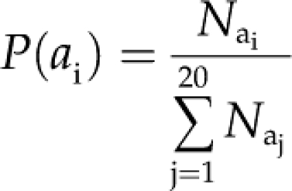
Simple Amino Acid Composition. Amino acid composition is the fraction of each amino acid in a protein sequence. The fraction of all the natural 20 amino acids was calculated using the following equation:

(1)

where P(a_i) is the fraction of a_i amino acid, N_ai is the total number of a_i amino acid, and the denominator represents the total number of amino acids in a protein sequence.

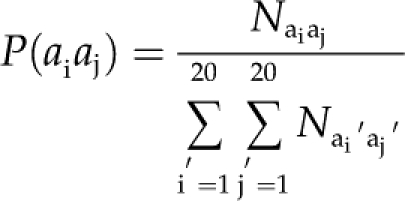
Dipeptide Composition. To encapsulate the global information about each protein sequence utilizing the sequence order effects, the dipeptide composition was calculated. This representation, which gives a fixed pattern length of 400 (20 × 20), encompasses the information of the amino acid composition along with the local order of amino acids. The fraction of each dipeptide was calculated according to the equation:

(2)

where P(a_ia_j) is the fraction of each a_ia_j dipeptide, N_aiaj is the total number of a_ia_j dipeptides, and the denominator represents the total number of all possible dipeptides.

Split Amino Acid Composition Technique

Terminal-Based N-Center-C (Three-Part) Composition. Many proteins in the cell contain important signal peptides at their N- or C-terminal region, which determine the subcellular location of the protein. It is not a simple task to directly identify these signal peptides from the sequence. Instead, this module calculated the amino acid composition separately from the N-terminal region, the C-terminal region, and the remaining center portion. For each part, a 20-D vector was extracted using Equation 1, so the combined feature vector of this module had 60 dimensions. The rationale behind using this type of approach is the fact that percentage composition of a whole sequence does not give adequate weight to the compositional bias, which is known to be present in the protein terminus. Separate SVM modules were developed by altering the various levels of N- and C-terminal residue length (10, 15, 20, 25, and 30 amino acids) in order to achieve maximum accuracy. However, residue length = 25 was found to be the best compromise and was used further in the development of the final method.

Four-Part Composition. This module assumed that different segments of a sequence can provide complementary information about the subcellular localization. It divided the query sequence into several fragments with equal length (four parts in this case) and calculated the amino acid composition (using Eq. 1) from the corresponding fragments separately. All the 20-D vectors from different segments were concatenated to form the final 80-D feature vector. This type of approach has comparatively shown some good results in earlier studies (Xie et al., 2005; Guo et al., 2006).

Similarity Search-Based PSI-BLAST Module

PSI-BLAST is a tool that produces a PSSM constructed from a multiple alignment of the top-scoring BLAST responses to a given query sequence (Altschul et al., 1997). This scoring matrix produces a profile designed to identify the key positions of conserved amino acids within a motif. When a profile is used to search a database, it can often detect subtle relationships between proteins that are distant structural or functional homologs. These relationships are often not detected by a BLAST search with a sample sequence query. Therefore, in this study, we used PSI-BLAST instead of normal standard BLAST because it has the capability to detect remote homologies. A module AtPSI-BLAST was designed in which a query sequence was searched against the entire Swiss-Prot database using PSI-BLAST. It carried out an iterative search in which the sequences found in one round were used to build score models for the next round of searching. Three iterations of PSI-BLAST were carried out at a cutoff E value of 0.001 (other levels of E value were also tried, but E = 0.001 was found to be the best compromise). This module could predict any of the seven localizations under study (chloroplast, cytoplasm, Golgi apparatus, mitochondrion, extracellular/secreted, nucleus, and plasma membrane) depending upon the similarity of the query protein to the proteins in the data set. If the top hits were more than 90% identical with the query, they were discarded, and then the annotation of the (sub)top hit was used as the predicted site of the query. The module would return “unknown subcellular localization” if no significant similarity was found.

Evolutionary Information-Based PSSM Module

PSI-BLAST is a strong measure of residue conservation in a given location. In the absence of any alignments, PSI-BLAST simply returns a 20-dimensional vector representing probabilities of conservation against mutations to 20 different amino acids, including itself. A matrix consisting of such vector representations for all the residues in a given sequence is called the PSSM. When a residue is conserved through cycles of PSI-BLAST, it is likely to be due to a purpose (i.e. biological function), and that is why it represents the evolutionary information of a protein sequence. The idea of adopting PSSM extracted from sequence profiles generated by PSI-BLAST as input information was first proposed by Jones (1999). This information is expressed in a position-specific scoring table (profile), which is created from a group of sequences previously aligned by PSI-BLAST against the nonredundant database at GenBank. The PSSM provides a matrix of dimension L rows and 20 columns for a protein chain of L amino acid residues, where 20 columns represent the occurrence/substitution of each type of 20 amino acids. It gives the log-odds score for finding a particular matching amino acid in a target sequence. This approach differs from other methods of sequence comparison in common use because any number of known sequences can be used to construct the profile, allowing more information to be used in testing of the target sequence. After that, every element in this matrix is divided by the length of the sequence and then scaled to the range of 0 to 1 using the standard linear function:

(3)

where X is the individual PSSM score of each amino acid in the matrix, Min_val is the minimum value in the PSSM matrix, and Max_val is the maximum value in the PSSM matrix.

Finally, this PSSM was used to generate a 400-dimensional input vector to the SVM by summing up all rows in the PSSM corresponding to the same amino acid in the primary sequence. The detailed process of converting an L × 20 size PSSM matrix into a 400-D input vector is diagrammatically shown in Figure 6.

Figure 6.

Schematic representation of the algorithm used to convert L × 20 size PSSM matrix into a 400-D input vector. The PSSM provides a matrix of dimension L rows and 20 columns for a protein chain of L amino acid residues, where 20 columns represent the occurrence/substitution of each type of 20 amino acids. [See online article for color version of this figure.]

Hybrid Technique Including a Novel Hybrid Approach Developed

Methodologies such as “hybrids” are devised to acquire more comprehensive information about the proteins by combining various features of a protein sequence. We developed various hybrid classifiers exploring different features of a protein sequence in different combinations to enhance the prediction accuracy. For example, at first we combined the 20-D vector of amino acid composition with the 400-D vector of dipeptide composition to form a 420-D input feature vector for SVM to develop the first hybrid classifier. In this way, we intended to combine the compositional information with the sequence order effects of a protein sequence to capture more comprehensive information, leading to enhanced accuracy. Similarly, many other combinations were attempted to extract more and more diverse information from the protein sequences (Fig. 5) and used in SVM for training the classifiers to achieve maximum accuracy. The PSI-BLAST output was also used in developing the hybrid classifiers by converting it to binary variables using the representations in Table IX. In fact, using such binary variables from similarity search output along with some other important features of a protein sequence resulted in dramatic improvement of the prediction accuracy. For example, the novel and smart combination of the 20-D amino acid composition, the terminal information-based 60-D composition vector, the evolutionary information-based 400-D PSSM vector, along with the above-mentioned 8-D PSI-BLAST output vector led to a significant increase in the prediction accuracy (for details, see “Results”).

Table IX. PSI-BLAST output as binary variables.

Location	Encoding Vector
Chloroplast	1 0 0 0 0 0 0 0
Cytoplasm	0 1 0 0 0 0 0 0
Golgi apparatus	0 0 1 0 0 0 0 0
Mitochondria	0 0 0 1 0 0 0 0
Extracellular	0 0 0 0 1 0 0 0
Nucleus	0 0 0 0 0 1 0 0
Plasma membrane	0 0 0 0 0 0 1 0
Unknown	0 0 0 0 0 0 0 1

Performance Evaluation

In the training of SVMs, we used the method of one versus the others or one versus the rest. For example, an SVM for the chloroplast protein group was trained with the chloroplast protein sequences used as positive samples and proteins in the other six subcellular location groups used as negative samples, because SVMs basically train classifiers between only two different samples. Thus, we built 105 SVM classifiers corresponding to seven subcellular localizations under 15 different types of approaches followed as discussed above. For each of these 15 different approaches, a query protein was tested against seven SVM classifiers to give seven prediction scores against each query protein.

The next step is to evaluate the performance of each classifier. As we developed a number of classifiers in this study, it is important to define the evaluation criteria precisely for better comparison. Most of the information retrieval papers report precision and recall, while bioinformatics, medical, and machine learning papers tend to report sensitivity and specificity apart from the MCC. We included all of them and added one more statistic, “error rate,” to the existing evaluation features. Sensitivity was calculated as TP/(TP + FN), where true positives (TP) were the number of labels correctly predicted as L_k for class k that were actually labeled L_k, and false negatives (FN) were the number of labels incorrectly predicted as not L_k that were actually labeled L_k. It is also sometimes referred to as “recall,” defined as the percentage of positively labeled instances that were predicted as positive. Specificity is another statistic, defined as the percentage of negatively labeled instances that were predicted as negative; this was calculated as TN/(TN + FP), where true negatives (TN) were the number of labels correctly predicted as not L_k that were actually not labeled L_k, and false positives (FP) were the number of labels incorrectly predicted as L_k that were actually not labeled as L_k. However, specificity is not as informative as precision for multi-labeled (nonbinary) classifiers. Therefore, it is always useful to include precision, which tells us about the percentage of positive predictions that are correct, calculated as TP/(TP + FP). Keeping in view the biological applications, we included another important statistic in this study: error rate gave us an idea about total percentage of wrong predictions, calculated as (FP + FN)/(TP + TN + FP + FN). The lower the error rate, the better the prediction classifier. The MCC is another measure used in machine learning for judging the quality of binary (two-class) as well as multi-labeled classifications. It takes into account the true and false positives and negatives and is generally regarded as a balanced measure that can be used even if the classes are of very different sizes. It returns a value between −1 and +1. A coefficient of +1 represents a perfect prediction, 0 represents an average random prediction, and −1 represents an inverse prediction. The MCC was calculated as:

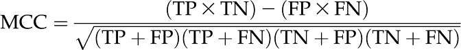(4)

In this way, the total number of TP, TN, FP, and FN were calculated from the scoring matrix in row-wise sorting, as followed by many other researchers (Hua and Sun, 2001; Bhasin and Raghava, 2004; Garg et al., 2005; Xie et al., 2005; Guo et al., 2006; Kaundal and Raghava, 2009): that is, an unknown or test protein sequence was classified into a particular localization class that corresponded to the highest output SVM score predicted from each of the seven models and ultimately calculated the sensitivity (recall), specificity, precision, error rate, and MCC values. An overall version of each statistic computed as its weighted average was also presented for judging the overall performance of the classifier(s). See Table I for the best classifier’s statistics and Supplemental Tables S7a to S20a for detailed performance comparisons of other developed classifiers.

RI and ROC Curves

RI is an important measure that provides the user more information as well as confidence about the quality of prediction. RI is assigned according to the difference (Δ) between the highest and second highest SVM output scores. We calculated the RI for our best classifier (AA+PSSM+N-Center-C+PSI-BLAST hybrid), adopting the strategy introduced by Hua and Sun (2001) and later followed by many other researchers, using Equation 5:

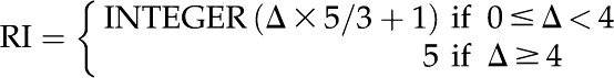(5)

To characterize the prediction performance for individual locations, we used ROC plot analysis (Swets, 1988; Zweig and Campbell, 1993). The ROC curve is a plot of sensitivity and specificity (or false positive rate = 1 − specificity) that shows the tradeoff between sensitivity and specificity. A ROC space is defined by 1 − specificity and sensitivity as x and y axes, respectively, which depicts relative tradeoffs between true positives and false positives. Each prediction result or one instance represents one point in the ROC space, which is determined by setting a threshold value. Plotting these ROC points for each possible threshold value resulted in a curve. The ROC curves of each location for our best classifier are presented in Figure 4.

Comparison with Other Prediction Programs

We compared the performance of AtSubP on two diverse Arabidopsis-specific independent data sets (I and II) with some of the widely used tools, such as TargetP (Emanuelsson et al., 2000), LOCtree (Nair and Rost, 2005), PA-SUB (Lu et al., 2004), MultiLoc (Höglund et al., 2006), WoLF PSORT (Horton et al., 2007), and Plant-PLoc (Chou and Shen, 2007b). Although technically, the comparison with other methods might not be fair, as each of these methods was developed with different sets of training data, our main emphasis was to demonstrate how these general tools performed for individual genome annotation (e.g. in this case, the performance of independent Arabidopsis test data sets on these methods compared with the developed species-specific one).

Annotation of the Arabidopsis Proteome

Currently, subcellular targeting prediction information is only available for one program (TargetP) on the TAIR Web site, while subcellular proteome information is limited and not accessible as defined sets. Keeping this in view, we performed predictions on the whole Arabidopsis proteome with our best classifier for all seven subcellular classes under study and provided these sets on our Web server. A total of 27,379 protein sequences were downloaded from TAIR release 9. As we got the hybrid-based (AA+PSSM+N-Center-C+PSI-BLAST) SVM model as our best performing classifier from this study, at first we separately generated the amino acid composition, PSSM matrix (the most time-consuming part), N-Center-C composition, and PSI-BLAST output for all 27,379 proteins. The amino acid-based conversion generated a 20-D vector, PSSM a 400-D vector, N-Center-C a 60-D vector, and PSI-BLAST an 8-D input vector (for details, see “Features and Modules” above). For each sequence, we then combined these vectors to form a hybrid 488-D input vector and ran it on the seven prediction models already generated to get seven corresponding SVM predicted scores for each sequence. For highly reliable and accurate predictions, we put various levels of threshold values (greater than 0.0, 0.1, 0.2, 0.3, 0.4, 0.5, 0.6, 0.7, 0.8, 0.9, and 1.0) on the final sorted score for each subcellular class. For example, if the maximum score of a query protein was found for the chloroplast category, in the next step we checked whether this score was more than the threshold value or not. Only then did we declare the query protein as predicted to be chloroplast. Therefore, one can say that the higher the threshold value, the more reliable the prediction. Furthermore, we cross-matched our high-confidence predictions (greater than 1.0 cutoff) with the available Swiss-Prot and TAIR annotations to judge the accuracy and reliability of these predictions.

Supplemental Data

The following materials are available in the online version of this article.

• Supplemental Figure S1. Comparison of overall amino acid composition across various eukaryotes.

• Supplemental Figure S2. Average amino acid composition of Arabidopsis mTPs compared with other eukaryotes.

• Supplemental Figure S3. Comparison of mTPs based on the electrostatic properties of their side chains.

• Supplemental Figure S4. Average amino acid composition of cytoplasm-localized proteins.

• Supplemental Figure S5. Average amino acid composition of nucleus-localized proteins.

• Supplemental Figure S6. RI curves based on 5-fold cross-validation performance.

• Supplemental Figure S7. ROC curves based on 5-fold cross-validation performance.

• Supplemental Table S1. P values for statistical test of significance.

• Supplemental Table S2. Distribution of Arabidopsis sequences used in 5-fold training/testing.

• Supplemental Table S3. Distribution of Arabidopsis sequences used for independent testing.

• Supplemental Table S4. a, All-Plant data set from Swiss-Prot; b, performance comparison of amino acid composition-based module from Arabidopsis-specific and All-Plant data on independent test set.

• Supplemental Table S5. Performance of best classifier for All-Plant method.

• Supplemental Table S6. Distribution of sequences within each localization across various eukaryotes.

• Supplemental Table S7. Performance of amino acid composition-based classifier developed from (a) Arabidopsis-specific data set and (b) All-Plant data set.

• Supplemental Table S8. Performance of dipeptide composition-based classifier from (a) Arabidopsis-specific data set and (b) All-Plant data set.

• Supplemental Table S9. Performance of N-Center-C composition-based classifier from (a) Arabidopsis-specific data set and (b) All-Plant data set.

• Supplemental Table S10. Performance of four-part composition-based classifier from (a) Arabidopsis-specific data set and (b) All-Plant data set.

• Supplemental Table S11. Performance of similarity-based PSI-BLAST module developed from (a) Arabidopsis-specific data set and (b) All-Plant data set.

• Supplemental Table S12. Performance of PSSM-based classifier from (a) Arabidopsis-specific data set and (b) All-Plant data set.

• Supplemental Table S13. Performance of AA+Dipeptide hybrid classifier from (a) Arabidopsis-specific data set and (b) All-Plant data set.

• Supplemental Table S14. Performance of AA+PSSM hybrid classifier from (a) Arabidopsis-specific data set and (b) All-Plant data set.

• Supplemental Table S15. Performance of AA+PSI-BLAST hybrid classifier from (a) Arabidopsis-specific data set and (b) All-Plant data set.

• Supplemental Table S16. Performance of AA+Dipep+PSI-BLAST hybrid classifier from (a) Arabidopsis-specific data set and (b) All-Plant data set.

• Supplemental Table S17. Performance of AA+PSSM+PSI-BLAST hybrid classifier from (a) Arabidopsis-specific data set and (b) All-Plant data set.

• Supplemental Table S18. Performance of AA+Dipep+N-Center-C+PSI-BLAST hybrid classifier from (a) Arabidopsis-specific data set and (b) All-Plant data set.

• Supplemental Table S19. Performance of AA+Dipep+Four-parts+PSI-BLAST hybrid classifier from (a) Arabidopsis-specific data set and (b) All-Plant data set.

• Supplemental Table S20. Performance of AA+PSSM+Four-parts+PSI-BLAST hybrid classifier developed from (a) Arabidopsis-specific data set and (b) All-Plant data set.

• Supplemental Table S21. Testing on GFP data (AtSubP versus TargetP).

• Supplemental Table S22. List of TAIR IDs where AtSubP predicts correctly in the absence of similarity-based information.

• Supplemental Materials and Methods S1. Detailed procedure for compiling and creating benchmark data sets.

References

- Altschul SF, Madden TL, Schäffer AA, Zhang J, Zhang Z, Miller W, Lipman DJ. (1997) Gapped Blast and PSI-Blast: a new generation of protein database search programs. Nucleic Acids Res 25: 3389–3402 [DOI] [PMC free article] [PubMed] [Google Scholar]
- Andersen JS, Mann M. (2006) Organellar proteomics: turning inventories into insights. EMBO Rep 7: 874–879 [DOI] [PMC free article] [PubMed] [Google Scholar]
- Andrade MA, O’Donoghue SI, Rost B. (1998) Adaptation of protein surfaces to subcellular location. J Mol Biol 276: 517–525 [DOI] [PubMed] [Google Scholar]
- Bhasin M, Raghava GPS. (2004) ESLpred: SVM-based method for subcellular localization of eukaryotic proteins using dipeptide composition and PSI-BLAST. Nucleic Acids Res 32: 414–419 [DOI] [PMC free article] [PubMed] [Google Scholar]
- Bogatyreva NS, Finkelstein AV, Galzitskaya OV. (2006) Trend of amino acid composition of proteins of different taxa. J Bioinform Comput Biol 4: 597–608 [DOI] [PubMed] [Google Scholar]
- Brown JWS, Shaw PJ, Shaw P, Marshall DF. (2005) Arabidopsis nucleolar protein database (AtNoPDB). Nucleic Acids Res 33: D633–D636 [DOI] [PMC free article] [PubMed] [Google Scholar]
- Brown MPS, Grundy WN, Lin D, Cristianini N, Sugnet CW, Furey TS, Ares M, Haussler D. (2000) Knowledge-based analysis of microarray gene expression data by using support vector machines. Proc Natl Acad Sci USA 97: 262–267 [DOI] [PMC free article] [PubMed] [Google Scholar]
- Byvatov E, Schneider G. (2003) Support vector machine applications in bioinformatics. Appl Bioinformatics 2: 67–77 [PubMed] [Google Scholar]
- Campbell WH, Gowri G. (1990) Codon usage in higher plants, green algae, and cyanobacteria. Plant Physiol 92: 1–11 [DOI] [PMC free article] [PubMed] [Google Scholar]
- Cedano J, Aloy P, Perez-Pons JA, Querol E. (1997) Relation between amino acid composition and cellular location of proteins. J Mol Biol 266: 594–600 [DOI] [PubMed] [Google Scholar]
- Chou KC, Shen HB. (2006) Hum-PLoc: a novel ensemble classifier for predicting human protein subcellular localization. Biochem Biophys Res Commun 347: 150–157 [DOI] [PubMed] [Google Scholar]
- Chou KC, Shen HB. (2007a) Recent progress in protein subcellular location prediction. Anal Biochem 370: 1–16 [DOI] [PubMed] [Google Scholar]
- Chou KC, Shen HB. (2007b) Large-scale plant protein subcellular location prediction. J Cell Biochem 100: 665–678 [DOI] [PubMed] [Google Scholar]
- Cortes C, Vapnik V. (1995) Support vector networks. Mach Learn 20: 273–293 [Google Scholar]
- Dunkley TP, Hester S, Shadforth IP, Runions J, Weimar T, Hanton SL, Griffin JL, Bessant C, Brandizzi F, Hawes C, et al. (2006) Mapping the Arabidopsis organelle proteome. Proc Natl Acad Sci USA 103: 6518–6523 [DOI] [PMC free article] [PubMed] [Google Scholar]
- Emanuelsson O. (2002) Predicting protein subcellular localisation from amino acid sequence information. Brief Bioinform 3: 361–376 [DOI] [PubMed] [Google Scholar]
- Emanuelsson O, Nielsen H, Brunak S, von Heijne G. (2000) Predicting subcellular localization of proteins based on their N-terminal amino acid sequence. J Mol Biol 300: 1005–1016 [DOI] [PubMed] [Google Scholar]
- Fennoy SL, Bailey-Serres J. (1993) Synonymous codon usage by maize nuclear genes is constrained by GC-biased mutation pressure and protein function. Nucleic Acids Res 21: 5294–5300 [DOI] [PMC free article] [PubMed] [Google Scholar]
- Garg A, Bhasin M, Raghava GPS. (2005) Support vector machine-based method for subcellular localization of human proteins using amino acid compositions, their order, and similarity search. J Biol Chem 280: 14427–14432 [DOI] [PubMed] [Google Scholar]
- Geldner N, Dénervaud-Tendon V, Hyman DL, Mayer U, Stierhof YD, Chory J. (2009) Rapid, combinatorial analysis of membrane compartments in intact plants with a multi-color marker set. Plant J 59: 169–178 [DOI] [PMC free article] [PubMed] [Google Scholar]
- Guo J, Lin Y, Liu X. (2006) GNBSL: a new integrative system to predict the subcellular location for gram-negative bacteria proteins. Proteomics 6: 5099–5105 [DOI] [PubMed] [Google Scholar]
- Heazlewood JL, Tonti-Filippini J, Verboom RE, Millar AH. (2005) Combining experimental and predicted data sets for determination of the subcellular location of proteins in Arabidopsis. Plant Physiol 139: 598–609 [DOI] [PMC free article] [PubMed] [Google Scholar]
- Heazlewood JL, Tonti-Filippini JS, Gout AM, Day DA, Whelan J, Millar AH. (2004) Experimental analysis of the Arabidopsis mitochondrial proteome highlights signaling and regulatory components, provides assessment of targeting prediction programs, and indicates plant-specific mitochondrial proteins. Plant Cell 16: 241–256 [DOI] [PMC free article] [PubMed] [Google Scholar]
- Höglund A, Dönnes P, Blum T, Adolph HW, Kohlbacher O. (2006) MultiLoc: prediction of protein subcellular localization using N-terminal targeting sequences, sequence motifs and amino acid composition. Bioinformatics 22: 1158–1165 [DOI] [PubMed] [Google Scholar]
- Horton P, Park KJ, Obayashi T, Fujita N, Harada H, Adams-Collier CJ, Nakai K. (2007) WoLF PSORT: protein localization predictor. Nucleic Acids Res 35: W585–W587 [DOI] [PMC free article] [PubMed] [Google Scholar]
- Hosmer DW, Lemeshow S. (2000) Applied Logistic Regression, Ed 2 John Wiley & Sons, New York, pp 156–164 [Google Scholar]
- Hua S, Sun Z. (2001) Support vector machine approach for protein subcellular localization prediction. Bioinformatics 17: 721–728 [DOI] [PubMed] [Google Scholar]
- Huang Y, Niu B, Gao Y, Fu L, Li W. (2010) CD-HIT Suite: a Web server for clustering and comparing biological sequences. Bioinformatics 003: 1–3 [DOI] [PMC free article] [PubMed] [Google Scholar]
- Huh WK, Falvo JV, Gerke LC, Carroll AS, Howson RW, Weissman JS, O’Shea EK. (2003) Global analysis of protein localization in budding yeast. Nature 425: 686–691 [DOI] [PubMed] [Google Scholar]
- Joachims T. (1999) Making large-scale SVM learning practical. Schölkopf B, Burges C, Smola A, , Advances in Kernel Methods: Support Vector Learning. MIT Press, Cambridge, MA, pp 41–56 [Google Scholar]
- Jones DT. (1999) Protein secondary structure prediction based on position-specific scoring matrices. J Mol Biol 292: 195–202 [DOI] [PubMed] [Google Scholar]
- Karlin S, Brocchieri L, Bergman A, Mrazek J, Gentles AJ. (2002) Amino acid runs in eukaryotic proteomes and disease associations. Proc Natl Acad Sci USA 99: 333–338 [DOI] [PMC free article] [PubMed] [Google Scholar]
- Kaundal R, Kapoor AS, Raghava GPS. (2006) Machine learning techniques in disease forecasting: a case study on rice blast prediction. BMC Bioinformatics 7: 485. [DOI] [PMC free article] [PubMed] [Google Scholar]
- Kaundal R, Raghava GPS. (2009) RSLpred: an integrative system for predicting subcellular localization of rice proteins combining compositional and evolutionary information. Proteomics 9: 2324–2342 [DOI] [PubMed] [Google Scholar]
- Kleffmann T, Russenberger D, von Zychlinski A, Christopher W, Sjölander K, Gruissem W, Baginsky S. (2004) The Arabidopsis thaliana chloroplast proteome reveals pathway abundance and novel protein functions. Curr Biol 14: 354–362 [DOI] [PubMed] [Google Scholar]
- Koroleva OA, Tomlinson ML, Leader D, Shaw P, Doonan JH. (2005) High-throughput protein localization in Arabidopsis using Agrobacterium-mediated transient expression of GFP-ORF fusions. Plant J 41: 162–174 [DOI] [PubMed] [Google Scholar]
- Li SJ, Ehrhardt DW, Rhee SY. (2006) Systematic analysis of Arabidopsis organelles and a protein localization database for facilitating fluorescent tagging of full-length Arabidopsis proteins. Plant Physiol 141: 527–539 [DOI] [PMC free article] [PubMed] [Google Scholar]
- Liu Q, Xue Q. (2005) Comparative studies on codon usage pattern of chloroplasts and their host nuclear genes in four plant species. J Genet 84: 55–62 [DOI] [PubMed] [Google Scholar]
- Lobry JR. (1997) Influence of genomic G+C content on average amino-acid composition of proteins from 59 bacterial species. Gene 205: 309–316 [DOI] [PubMed] [Google Scholar]
- Lu Z, Szafron D, Greiner R, Lu P, Wishart DS, Poulin B, Anvik J, Macdonell C, Eisner R. (2004) Predicting subcellular localization of proteins using machine-learned classifiers. Bioinformatics 20: 547–556 [DOI] [PubMed] [Google Scholar]
- Michaud GA, Snyder M. (2002) Proteomic approaches for the global analysis of proteins. Biotechniques 33: 1308–1316 [DOI] [PubMed] [Google Scholar]
- Mott R, Schultz J, Bork P, Ponting CP. (2002) Predicting protein cellular localization using a domain projection method. Genome Res 12: 1168–1174 [DOI] [PMC free article] [PubMed] [Google Scholar]
- Nair R, Rost B. (2005) Mimicking cellular sorting improves prediction of subcellular localization. J Mol Biol 348: 85–100 [DOI] [PubMed] [Google Scholar]
- Nakashima H, Nishikawa K. (1994) Discrimination of intracellular and extracellular proteins using amino acid composition and residue-pair frequencies. J Mol Biol 238: 54–61 [DOI] [PubMed] [Google Scholar]
- Pan SQ, Carter CJ, Raikhel NV. (2005) Understanding protein trafficking in plant cells through proteomics. Expert Rev Proteomics 2: 781–792 [DOI] [PubMed] [Google Scholar]
- Park KJ, Kanehisa M. (2003) Prediction of protein subcellular locations by support vector machines using compositions of amino acids and amino acid pairs. Bioinformatics 19: 1656–1663 [DOI] [PubMed] [Google Scholar]
- Pe’er I, Felder CE, Man O, Silman I, Sussman JL, Beckmann JS. (2004) Proteomic signatures: amino acid and oligopeptide compositions differentiate among phyla. Proteins 54: 20–40 [DOI] [PubMed] [Google Scholar]
- Peng WM, Rajapakse JC. (2005) Multi-class protein subcellular localization prediction using support vector machines. Proc IEEE Symp 14: 1–8 [Google Scholar]
- Rashid M, Saha S, Raghava GPS. (2007) Support vector machine-based method for predicting subcellular localization of mycobacterial proteins using evolutionary information and motifs. BMC Bioinformatics 8: 337. [DOI] [PMC free article] [PubMed] [Google Scholar]
- Rey S, Gardy JL, Brinkman FSL. (2005) Assessing the precision of high-throughput computational and laboratory approaches for the genome-wide identification of protein subcellular localization in bacteria. BMC Genomics 6: 162. [DOI] [PMC free article] [PubMed] [Google Scholar]
- Rhee SY, Beavis W, Berardini TZ, Chen G, Dixon D, Doyle A, Garcia-Hernandez M, Huala E, Lander G, Montoya M, et al. (2003) The Arabidopsis Information Resource (TAIR): a model organism database providing a centralized, curated gateway to Arabidopsis biology, research materials and community. Nucleic Acids Res 31: 224–228 [DOI] [PMC free article] [PubMed] [Google Scholar]
- Sandberg R, Branden CI, Ernberg I, Coster J. (2003) Quantifying the species-specificity in genomic signatures, synonymous codon choice, amino acid usage and G+C content. Gene 311: 35–42 [DOI] [PubMed] [Google Scholar]
- Sarda D, Chua GH, Li KB, Tang F, Krishnan A. (2005) pSLIP: SVM based protein subcellular localization prediction using multiple physicochemical properties. BMC Bioinformatics 6: 152. [DOI] [PMC free article] [PubMed] [Google Scholar]
- Schneider G, Fechner U. (2004) Advances in the prediction of protein targeting signals. Proteomics 4: 1571–1580 [DOI] [PubMed] [Google Scholar]
- Scott MS, Thomas DY, Hallett MT. (2004) Predicting subcellular localization via protein motif co-occurrence. Genome Res 14: 1957–1966 [DOI] [PMC free article] [PubMed] [Google Scholar]
- Sun Q, Zybailov B, Majeran W, Friso G, Olinares PDB, van Wijk KJ. (2008) PPDB, the Plant Proteomics Database at Cornell. Nucleic Acids Res 37: D969–D974 [DOI] [PMC free article] [PubMed] [Google Scholar]
- Swets JA. (1988) Measuring the accuracy of diagnostic systems. Science 240: 1285–1293 [DOI] [PubMed] [Google Scholar]
- Taylor SW, Fahy E, Ghosh SS. (2003) Global organellar proteomics. Trends Biotechnol 21: 82–88 [DOI] [PubMed] [Google Scholar]
- Tekaia F, Yeramian E. (2006) Evolution of proteomes: fundamental signatures and global trends in amino acid compositions. BMC Genomics 7: 307. [DOI] [PMC free article] [PubMed] [Google Scholar]
- Tekaia F, Yeramian E, Dujon B. (2002) Amino acid composition of genomes, lifestyles of organisms, and evolutionary trends: a global picture with correspondence analysis. Gene 297: 51–60 [DOI] [PubMed] [Google Scholar]
- Tian GW, Mohanty A, Chary SN, Li S, Paap B, Drakakaki G, Kopec CD, Li J, Ehrhardt D, Jackson D, et al. (2004) High-throughput fluorescent tagging of full-length Arabidopsis gene products in planta. Plant Physiol 135: 25–38 [DOI] [PMC free article] [PubMed] [Google Scholar]
- Vapnik V. (1995) The Nature of Statistical Learning Theory. Springer, New York [Google Scholar]
- Ward JJ, McGuffin LJ, Buxton BF, Jones DT. (2003) Secondary structure prediction with support vector machines. Bioinformatics 19: 1650–1655 [DOI] [PubMed] [Google Scholar]
- Wiwatwattana N, Kumar A. (2005) Organelle DB: a cross-species database of protein localization and function. Nucleic Acids Res 33: D598–D604 [DOI] [PMC free article] [PubMed] [Google Scholar]
- Xie D, Li A, Wang M, Fan Z, Feng H. (2005) LOCSVMPSI: a Web server for subcellular localization of eukaryotic proteins using SVM and profile of PSI-BLAST. Nucleic Acids Res 33: 105–110 [DOI] [PMC free article] [PubMed] [Google Scholar]
- Zweig MH, Campbell G. (1993) Receiver-operating characteristic (ROC) plots: a fundamental evaluation tool in clinical medicine. Clin Chem 39: 561–577 [PubMed] [Google Scholar]
Associated Data
This section collects any data citations, data availability statements, or supplementary materials included in this article.