CuBIC: cumulant based inference of higher-order correlations in massively parallel spike trains

Abstract

Recent developments in electrophysiological and optical recording techniques enable the simultaneous observation of large numbers of neurons. A meaningful interpretation of the resulting multivariate data, however, presents a serious challenge. In particular, the estimation of higher-order correlations that characterize the cooperative dynamics of groups of neurons is impeded by the combinatorial explosion of the parameter space. The resulting requirements with respect to sample size and recording time has rendered the detection of coordinated neuronal groups exceedingly difficult. Here we describe a novel approach to infer higher-order correlations in massively parallel spike trains that is less susceptible to these problems. Based on the superimposed activity of all recorded neurons, the cumulant-based inference of higher-order correlations (CuBIC) presented here exploits the fact that the absence of higher-order correlations imposes also strong constraints on correlations of lower order. Thus, estimates of only few lower-order cumulants suffice to infer higher-order correlations in the population. As a consequence, CuBIC is much better compatible with the constraints of in vivo recordings than previous approaches, which is shown by a systematic analysis of its parameter dependence.

Introduction

More than 50 years after its first conception (Hebb 1949), the idea that entities of thought or perception are represented by the coordinated activity of (large) neuronal groups has lost nothing of its attraction (e.g., Wennekers et al. 2003; Harris 2005; Sakurai and Takahashi 2006). Now known as the “assembly hypothesis”, the concept of a single, unified principle underlying such diverse computational tasks as association and pattern completion (e.g., Palm 1982), binding (e.g., Singer and Gray 1995), language processing (e.g., Wennekers et al. 2006), or memory formation and retrieval (e.g., Pastalkova et al. 2008) has inspired numerous theoretical and experimental neuroscientists. However, whether or not the dynamic formation of cell assemblies constitutes a fundamental principle of cortical information processing remains a controversial issue of current research (e.g., Singer 1999; Shadlen and Movshon 1999; van Vreeswijk 2006). While initially mainly technical problems limited the experimental surge for support of the assembly hypothesis (state-of-the-art electrophysiological setups in the last century allowed to record only few neurons simultaneously), the recent advent of multi-electrode array and optical imaging techniques reveals fundamental shortcomings of available analysis tools (Brown et al. 2004).

Based on the efficacy of synchronized presynaptic spikes to reliably generate output spikes (Abeles 1982; König et al. 1995; Diesmann et al. 1999), the temporal coordination of spike timing is a commonly accepted signature of assembly activity (e.g., Gerstein et al. 1989; Abeles 1991; Singer et al. 1997; Harris 2005). Consequently, approaches to detect assembly activity have focused on the detection of correlated spiking. Statistically, coordinated spiking of large neuronal groups has been associated to higher-order correlations among the corresponding spike trains (Martignon et al. 1995, 2000), where “genuine higher-order correlations” are assumed, if coincident spikes of a neuronal group cannot be explained/predicted by the firing rate and pairwise correlations alone. Mathematical frameworks for the estimation of such correlations exist (Nakahara and Amari 2002; Martignon et al. 1995; Schneider and Grün 2003; Gütig et al. 2003), however, run into combinatorial difficulties, as they assign one correlation parameter for each group of neurons and thus require in the order of 2^N parameters for a population of N simultaneously recorded neurons. Comparing the number of parameters to the available sample size of typical electrophysiological recordings (e.g. a population of N = 100 neurons implies ∼10³⁰ parameters while 100 s of data sampled at 10 kHz provide ∼10⁶ samples) illustrates the principal infeasibility of this approach. In fact, the estimation of such higher-order correlations runs into severe practical problems even for populations of N∼10 neurons (Martignon et al. 1995, 2000; Del Prete et al. 2004).

Due to the limitations of multivariate approaches, most studies in favor of cortical cell-assemblies resort to pairwise interactions. And indeed, the existence and functional relevance of pairwise interactions has been demonstrated in various cortical systems and behavioral paradigms (e.g., Eggermont 1990; Vaadia et al. 1995; Kreiter and Singer 1996; Riehle et al. 1997; Kohn and Smith 2005; Sakurai and Takahashi 2006; Fujisawa et al. 2008). However, although pairwise analysis can indicate highly correlated groups of neurons (Berger et al. 2007; Fujisawa et al. 2008), knowledge of higher-order correlations is essential to conclude on large, synchronously firing assemblies (see examples in Fig. 4 for illustration). The importance to transcend pairwise descriptions of parallel spike trains is further underscored by the strong impact of higher-order correlations on the dynamics of cortical neurons (e.g., Bohte et al. 2000; Kuhn et al. 2003). Taken together, we believe that the increasing number of simultaneously observable neurons can only be exploited by analysis techniques that go beyond mere pairwise correlations but are nevertheless applicable given the limited sample size of electrophysiological data (Brown et al. 2004).

Fig. 4.

CuBIC results for three example data sets with identical rates and pairwise correlations, but different higher-order correlations (each column shows one data set). Amplitude distributions (top, logarithmic y-scale) illustrate the correlation structure of the respective CPP. Below are the raster displays of the activities of N = 100 processes demonstrated for a period of the first 2 s of a total simulation time of T = 100 s. The third panels from top show the population spike counts of the data, computed with a bin width of h = 5 ms. Their histograms (of the total simulation time) are shown in the fourth panel as the complexity distribution Z (blue bars) and its logarithmically transformed version (green line graph, y-axis on the right). The bottom panels show the results of CuBIC, i.e. the p-values for subsequent hypothesis tests assuming increasingly higher ξ in the null-hypotheses . The left graph shows the results for the second cumulant (m = 2), the graph on the right uses the third cumulant (m = 3), respectively. Red filled circles denote p-values below a significance level of α = 0.05. Correlation in the data sets was induced by events of amplitude ξ _syn = 2 (Set1, left), ξ _syn = 7 (Set2, middle), and ξ _syn = 15 (Set3, right), that were injected in addition to the background spikes at ξ = 1. In all data sets, the carrier rate ν and the relative probabilities of events of amplitude 1 and ξ _syn were chosen to mimic N = 100 neurons with identical firing rates (10 Hz). We let 70 of those neurons fire independently (neuron IDs 1-70) and N _C = 30 to form a homogeneously correlated subgroup with a count-correlation coefficient of c = 0.01 (neuron IDs 71 - 100), yielding higher-order event rates of ν ₂ = 43.5 Hz in Set1, ν ₇ = 2.07 Hz in Set2 and ν ₁₅ = 0.41 Hz in Set3. Test parameters: α = 0.05, ξ _max = 15, m _max = 4

In this study, we present a novel cumulant based inference procedure for higher-order correlations (CuBIC). The method is specifically designed to detect the presence of higher-order correlations under the constraints of the limited sample size typical of standard experimental paradigms. This is achieved by combining three basic ideas. First, CuBIC is based on the binned and summed spiking activity across all recorded neurons (population spike count). This transforms the multivariate problem to estimate all ∼2^N model parameters into a parsimoniously parametrized univariate problem, thereby dramatically reducing the required sample size. Furthermore, pooling the spiking activity avoids the need for sorting the multi-unit spike trains recorded on a single electrode into isolated single neuron spike trains. Correlations among the individual spike trains are measured by the cumulants of the population spike count. Importantly, the cumulant correlations of higher order used here do not conform to the higher-order parameters of the exponential family used by, e.g., Schneidman et al. (2006). Second, we use the compound Poisson process (e.g., Snyder and Miller 1991; Daley and Vere-Jones 2005) as a flexible, intuitive, and analytically tractable model of correlated spiking activity. Here, correlations among spike trains are modeled by the insertion of additional coincident events in continuous time (Holgate 1964; Ehm et al. 2007; Johnson and Goodman 2008; Staude et al. 2010). As a consequence, the conceptual difference between the discretely sampled data (population spike count) and the continuous time spike trains is an explicit feature of the present framework. And third, we formalize the observation that even small correlations of lower order can imply synchronized spiking of large neuronal groups (Amari et al. 2003; Benucci et al. 2004; Schneidman et al. 2006).

The first and second ideas are elaborated in Section 2. Based on the compound Poisson process, Section 3 thoroughly formalizes the third idea, where we analytically derive confidence intervals for a hierarchy of statistical hypothesis tests. The tests are then combined to compute a lower bound for the order of correlations in a given data set . Importantly, the inferred lower bound can considerably exceed the order of the estimated correlations. Thereby, CuBIC avoids the direct estimation of higher-order correlations, which is practically infeasible for orders of , but nevertheless reveals their presence. As shown by extensive Monte Carlo simulations (Section 4), using the third cumulant suffices to reliably detect existing correlations of order > 10 in large neuronal pools (here N∼100 neurons with average count-correlation coefficients of c∼0.01). Thus, CuBIC achieves an unprecedented sensitivity for higher-order correlations in scenarios with reasonable sample sizes, i.e. experiment durations of T < 100 s. The Discussion section relates the cumulant-based correlations used here to the higher-order interaction parameters of the exponential family (e.g., Martignon et al. 1995; Nakahara and Amari 2002; Shlens et al. 2006) and critically discusses the implications of the hypothesized compound Poisson process. Preliminary results have been presented previously in abstract form (Staude et al. 2007).

Measurement & model

Measurement

Assume an observation of a large number of parallel spike trains. To measure correlation, we describe such a population as a succession of “patterns”, (T denotes transpose), one pattern for every time bin of width h. The components of X are the binned, discretized spike trains, i.e. X _i(s) is the spike count of the ith neuron in the interval [s,s + h). Given these patterns, we define the population spike count Z(s) at s as the total spike count in the sth bin (Fig. 1)

Fig. 1.

Schema of the compound Poisson process and its measurement. Left half: spike event times (horizontal bars) of individual neurons x ₁(t),...,x _N(t) and tick marks of the carrier process z(t) (top) with the associated amplitudes (numbers above the ticks), represented in continuous time. The population spike count Z(s) (below the spike trains) counts the number of spikes across all neurons in bins of width h (dotted lines). Right half: distribution of the amplitudes a _j of the carrier process z(t) (amplitude distribution f _A, top) and distribution of the population spike count Z(s) (complexity distribution f _Z, bottom, estimated from 100 s of data with the given amplitude distribution and a bin size of h = 5ms; dashed line: Poisson fit, corresponding to an independent population with the same firing rates). To construct a population of correlated spike trains, amplitudes a _j are drawn for all events t _j in the carrier process i.i.d from f _A. The individual processes x _i(t) are then constructed by copying every event at t _j of the carrier process z(t) into a _j “child” processes x _i(t) (the specific process IDs are here drawn randomly from {1,...,N}). Correlations of order ξ are induced, whenever events in the carrier process are copied into more than ξ processes, i.e. if the amplitude distribution assigns non-zero probabilities for amplitudes ≥ ξ (see Theorem 1 in Section 2.4)

The variable Z(s), from here on referred to as the “complexity” of the population at s, counts the number of spikes that fall into the interval [sh,(s + 1)h), irrespective of the neuron IDs that emitted these spikes. In the case where the X _i are binary (“1” for one or more spikes in the bin, “0” for no spike), Z(s) is simply the number of neurons that spike in the time slice. As opposed to most other frameworks for correlation analysis (e.g., Aertsen et al. 1989; Martignon et al. 1995; Grün et al. 2002a; Nakahara and Amari 2002; Shlens et al. 2006), however, the method presented in this study does not assume binary variables. As a consequence, our term “complexity” as the “number of spikes per bin in the population” does not comply with the “number of active neurons per bin” used in binary frameworks.

To regard the values of Z(s) in different bins as i.i.d. random variables, we here assume that Z(s) and Z(s + k) are independent for k ≠ 0 (zero memory), and that the distribution of Z(s) does not depend on the time bin s (stationarity). We name the resulting distribution of population spike counts

the “complexity distribution” of the population. The validity of these assumptions with respect to real spike trains, and potential adaptations of CuBIC, are discussed in Section 5.3.

Despite ignoring the specific neuron IDs that contribute to the patterns X(s), the complexity distribution nevertheless contains information about the correlation structure of the population. For instance, if the counting variables {X _i}_{i ∈ {1,...,N}} are independent Poisson counts, the corresponding population spike count, being the sum of the independent Poisson variables, is again a Poisson variable, and thus the complexity distribution f _Z is a Poisson distribution. Correlations change the relative probabilities for patterns of high and low complexities as compared to the independent case, as can be seen by comparing the complexity distribution of the correlated population and its independent Poisson fit in Fig. 1 (blue bars and dashed gray line, respectively; see also Grün et al. 2008a and Louis and Grün 2009). We quantify such deviations from independence by means of the cumulants κ _m[Z] of the population spike count Z.

Correlations and cumulants

Like the more familiar (raw) moments of a random variable Z, the cumulants κ _m[Z] characterize the shape of its distribution (see Appendix A and, e.g., Stratonovich 1967; Gardiner 2003). Most common are the first two cumulants, the expectation and the variance. These admit simple expressions in terms of the moments: and . Similar expressions for higher cumulants, however, are exceedingly complicated (see Stuart and Ord 1987 for explicit expressions for m ≤ 10).

The most important property of cumulants, and their advantage over the raw moments is that the cumulant of the sum of independent random variables is the sum of their cumulants. For m = 2 and , for instance, we have the well-known variance-covariance relationship

1

Equation (1) shows that if , which is the case if the X _i are (pairwise) uncorrelated. Cumulant correlations of higher order, the so-called “mixed” or “connected” cumulants, are a straightforward generalization of the covariance in exactly this sense: if the population has neither pairwise nor triple-wise cumulant correlations, then (see Appendix A for a concise definition, and Gardiner 2003, for a general introduction). Higher-order cumulant correlations generalize the covariance also with respect to the fact that implies . That is, if the multivariate random vector X decomposes into independent subgroups, then the cumulant correlations vanish (Streitberg 1990). For notational consistency, we will from now on stick to the cumulant notation, e.g., use “first/second cumulant” instead of the more familiar terms “mean/variance”.

A further consequence of Eq. (1) is that κ ₂[Z] is influenced only by the single process statistics (via ) and pairwise correlations (via ). No higher-order correlations contribute to the second cumulant. This holds also for higher cumulants, i.e. κ _m[Z] depends on correlations among the X _i of maximal order m. And finally, in the same way that κ ₂[Z] depends on pairwise correlations and the single process statistics, also κ _m[Z] does not measure pure mth order correlations, but depends on correlations of all orders up to m. While a correction of the second cumulant for the influence of the single process statistics would be straightforward (subtracting in Eq. (1), see Appendix B), correcting higher cumulants for the influence of correlations of lower order is exceedingly complicated. We therefore employ a parametric model for Z, the compound Poisson process (see next section), the parameters of which can be interpreted straightforwardly in terms of higher-order correlations among the X _i.

We would like to stress that the higher-order correlations defined by cumulants differ strongly from the higher-order parameters of the exponential family used by, e.g. Martignon et al. (1995), Nakahara and Amari (2002), Shlens et al. (2006). The relationship between these two frameworks is discussed in more detail in Section 5.1 (see also Staude et al. 2010).

Model

As opposed to the discretized, i.e. binned, population spike count Z(s) of the previous section, the proposed model operates in continuous, i.e. unbinned time. That is, we model the process , where denotes the ith unbinned, continuous-time spike train (i = 1,...,N) with spike-event times . The model we propose for z(t) is that of a compound Poisson process (CPP)

2

where the event times t _j constitute a Poisson process, and the marks a _j are i.i.d. integer-valued random variables, drawn independently for all t _j. The marks a _j determine the number of neurons that fire at time t _j, and will be referred to as the “amplitude” of the event at time t _j. The probability that an event has a specific amplitude is determined by the amplitude distribution f _A, i.e. (see Fig. 1). The Poisson process that generates the events t _j is called the “carrier process” of the model and its rate ν is the “carrier rate”. Processes of this type are also referred to as generalized, or marked, Poisson processes (see e.g. Snyder and Miller 1991 for a general definition and Ehm et al. 2007 for an application to spike train analysis).

To interpret the CPP as the lumped process of a correlated population of N spike trains, and to utilize the CPP for the generation of artificial data, the events of z(t) are assigned to individual processes x _i(t) (i = 1,...,N). The simplest model draws the a _j process IDs that receive a spike at t _j as a random subset from {1,...N}, independently for all event times t _j (Fig. 1). This results in a homogeneous population of correlated Poisson processes, where all processes have the same rate, all pairs of processes have identical correlations, and so on. The SIP/MIP models presented in Kuhn et al. (2003) are special cases of this more general model (see also Appendix B for examples). As the inference procedure CuBIC presented in the remainder of this study is based solely on the summed activity, however, it is not affected by the details of the copying procedure. In particular, CuBIC does not presuppose that the population is homogeneous.

Relating measurement and model

To interpret the continuous-time model parameters ν and f _A in terms of correlations among the counting variables X _i, we now relate the former to the cumulants of the population spike count Z. First of all, note that as the carriers process z(t) is a Poisson process, the population spike counts in different bins are i.i.d. For l = 1,...,N, define the processes y _l(t) that determine all event times t _j in Eq. (2) with given amplitude a _j = l (compare Appendix A). Then the CPP z(t) admits the representation . As a consequence, the discretized population spike count satisfies , where the Y _l are the counting variables obtained from the processes y _l(t) using a bin size h. As the event times t _j of z(t) follow a Poisson process and the subsequent amplitudes a _j are independent, the y _l(t) are independent Poisson processes. The rate ν _l of y _l(t) is given by ν _l = f _A(l)·ν (l = 1,2,...). Hence, the Y _l are Poisson variables with parameter ν _l h. As a consequence, all cumulants of Y _l are identical and given by κ _m[Y _l] = ν _l h (m = 1,2,...; Gardiner 2003). The scaling behavior of the cumulants for all m (Mattner 1999) yields

Using ν _l = f _A(l)·ν and , we finally have

3

Equation (3) is the central equation of this study and requires a few more remarks. First, it implies that the first two cumulants of the population spike count, κ ₁[Z] and κ ₂[Z], are determined solely by the carrier rate ν and the first two moments of the amplitude distribution, μ ₁[A] and μ ₂[A]. As κ ₁[Z] and κ ₂[Z] determine firing rates and pairwise correlations in the population (Appendix B, Eqs. (24) and (26)), we conclude that all CPP models with identical carrier rate ν and identical μ ₁[A] and μ ₂[A] generate populations with identical rates and pairwise correlations. Differences in higher-order correlations can thus be modeled by choosing different higher moments for f _A (see Section 2.4 for the precise relationship between the entries of the amplitude distribution and higher-order correlations in the population). This makes the CPP a very flexible and convenient model to generate artificial data sets with identical firing rates and pairwise correlations, yet different higher-order correlations (see Section 4 and Appendix B for examples, and Kuhn et al. 2003; Ehm et al. 2007; Staude et al. 2010 for alternative parametrizations).

Second, the moments of the strictly positive, integer-valued variable A increase with the order, i.e. satisfy μ _m[A] ≤ μ _m + 1[A] for m ≥ 1. By Eq. (3), this implies that also the cumulants of Z increase with the order, i.e. κ _m[Z] ≤ κ _m + 1[Z]. This is a reformulation of the fact that insertion of joint spikes as done in the CPP generates only positive correlations (e.g., Brette 2009; Johnson and Goodman 2008, Johnson and Goodman, unpublished manuscript), and it shows that certain combinations of cumulants cannot be realized by the CPP.

Terminology

The conceptual difference between the measured data (the counting variables X _i and the complexity distribution f _Z) and the parametric model that we assume to underlie this measurement (the CPP) is crucial for the remainder of this study. To illustrate this difference, note that f _Z depends on the bin size h used in the discretization. Larger bin widths increase the probabilities for high complexities, while smaller bin widths increase the probability for empty bins. The parameters of the CPP, on the other hand, do not change with the bin size. For instance, if all events of z(t) have amplitude a _j = 1, i.e. the amplitude distribution has a single peak at ξ = 1, the population consists of independent Poisson processes, irrespective of the bin size used for the analysis, or even the number of recorded neurons. In other words: patterns of complexity Z ≥ 2 can occur by chance, while events of amplitude ξ ≥ 2 do not occur by chance but imply correlations in the population. The order of the correlation, in turn, is determined by the amplitudes of the events in the corresponding CPP (see Appendix A for the proof):

Theorem 1

Let be a compound Poisson process with amplitude distribution f _A , and let be the vector of counting variables obtained from the x _i(t) with a bin width h . Then the components of X have correlations of order m if and only if f _A assigns non-zero probabilities to amplitudes ≥ m.

The above theorem confirms the intuitive conception that, within the framework of the CPP, correlations of a certain order m require injected coincidences into at least m processes (events of amplitudes ≥ m). Also, a population with only pairwise but no higher-order correlations has events of maximal amplitude m = 2. Importantly, correlations in the above theorem are defined strictly on the basis of the discretized counting variables X _i. As a consequence, they do not resolve (and do not depend on) the perfect temporal precision of the coincident events in the CPP: if the events of z(t) were copied into the individual processes with a temporal jitter that is small with respect to the bin size h, the correlations among the counting variables will hardly be affected (see Section 5.3.3 for a more detailed discussion). Note also that events of amplitude ξ induce not only correlations of order ξ, but also of orders < ξ.

Cumulant based inference of higher-order correlations (CuBIC)

This section describes our cumulant based inference procedure for higher-order correlations (CuBIC). The outcome of CuBIC is a lower bound on the order of correlation in the spiking activity of large groups of simultaneously recorded neurons. As will be shown in Section 4, this lower bound can exceed the order of the cumulants that were estimated for the inference. Thereby, CuBIC can provide statistical evidence for large correlated groups without the discouraging requirements on sample size that direct tests for higher-order correlations have to meet. This is achieved by exploiting constraining relations among correlations of different orders. For illustration, consider as an example the extreme situation of 4 simultaneously recorded neurons, where all neuron pairs have a correlation coefficient of c = 1. As c = 1 implies identity for all pairs of spike trains, all four spike trains of this example must be identical (Fig. 2, left). In other words, a spike in one neuron implies joint spike events in all the other neurons. Thus, the data must have correlation of order 4.

Fig. 2.

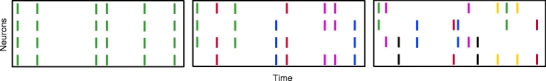
Strong pairwise correlations imply higher-order correlations. Raster plots show populations that have a single event amplitude that differs in the three panels (left: all events have amplitude 4, middle: amplitude 3, right: amplitude 2). Note that an increase in pairwise correlations in the right population can only be achieved by increasing the event amplitude and thereby the order of correlation. The plots thus illustrate the populations that are maximally correlated with correlations of order ≤ 4 (left), ≤ 3 (middle) and ≤ 2 (right)

The key observation of this example is that the order of correlation we inferred () exceeds the order m of the measured correlations (here m = 2). CuBIC formalizes this example in the framework of the CPP, and generalizes it in two aspects:

1. Assume the correlation coefficients had been somewhat smaller than 1: do we still need correlation of order 4 to explain the measured pairwise correlation? Or would correlation of order 3 as in Fig. 2, middle, or even of order 2 as in Fig. 2, right, suffice to explain the measured correlations? In other words: What order of correlation is minimally required to explain the measured pairwise correlations?

2. Can we formulate a similar reasoning for measured correlations of higher order? What order of correlation is minimally required to explain the measured correlations of third (fourth,...) order?

The next section details our approach to answer the first question. The results are then generalized to answer the second question (Section 3.2). Finally, we explain how CuBIC combines the results to infer a lower bound for the order of correlation in a given data set (Section 3.3).

Testing pairwise correlations (m = 2)

We approach the first aspect with a hierarchy of statistical hypothesis tests, labeled by the integer ξ. For fixed ξ, the null hypothesis states that the pairwise correlations (thus the superscript “2”) in the population are compatible with the assumption that there is no correlation beyond order ξ; the alternative states that correlation of order higher than ξ is necessary to explain the pairwise correlations. Rejection of e.g. in favor of thus implies the existence of correlation of at least order 5. The test statistics to decide between these alternatives is the second sample cumulant of the population spike count, and the compound Poisson process provides the framework to analytically derive the required confidence bounds.

The null hypothesis

The formulation of a null hypothesis requires a careful distinction between the random variable that describes the experiment, and the data sample that is tested against the hypothesis. For a fixed value of the test parameter ξ, this section formulates the null hypothesis , using the random variable Z′ that describes the population spike count of a neuronal population. Section 3.1.2 explains how a given data sample {Z′₁,...,Z′_L} is tested against .

The null hypotheses is based on the CPP model whose population spike count has the maximal second cumulant under the constraints that (a) the first cumulant equals that of a given population spike count Z′, and (b) the maximal order of correlation in the model is ξ. Using the amplitude distribution f _A to parametrize its correlation structure, this CPP model is the solution of the constrained maximization problem

4

where ν and f _A are the CPP parameters that determine the population spike count Z. We rewrite Eq. (4) by observing that the second constraint () together with Eq. (3) implies . With ν _l = f _A(l)·ν (Section 2.3), we thus have

5

where the dot denotes the standard scalar product. Using Eq. (5) and the vector notation and , the maximization problem of Eq. (4) becomes

6

In Eq. (6), both the function to maximize () and the constraint () depend linearly on the parameters . Problems of this type, so-called Linear Programming Problems, are uniquely solvable, e.g. using the Simplex Method (Press et al. 1992, Chapter 10.8). The solution yields the upper bound for the second cumulant and the corresponding parameter vector . The carrier rate and amplitude distribution of the CPP that maximizes Eq. (6) are then given by and .

Assume that the combination of firing rates and pairwise correlations in the population can be realized with correlations of order ≤ ξ. Then, the second cumulant of its population spike count Z′ must be smaller than the upper bound computed in the previous section. We thus formulate the null hypothesis

The alternative hypothesis

states that, within the framework of the CPP model, the pairwise correlations in the population imply the presence of correlation of order > ξ.

Test statistics and their distributions

The derivations in the previous section require the cumulants κ ₁[Z′] and κ ₂[Z′] of the random variable Z′. Given only a data sample {Z′₁,...,Z′_L} of size L, we estimate these quantities by the standard sample mean and (unbiased) sample variance (Stuart and Ord 1987)

The test of the data sample against requires the distribution of the test statistics k ₂ under the null hypothesis. To derive this distribution, recall that and , where the κ _i[Z′] are the unknown cumulants of the variable Z′ that underlies the sample (Stuart and Ord 1987). The trick of CuBIC is to assume in that Z′ is the population spike count of the CPP that solves Eq. (6) after the unknown cumulant κ ₁[Z′] has been substituted with its estimate k ₁. Under this assumption, all cumulants of Z′ can be computed by inserting the model parameters ν ^* and into Eq. (3), which yields

7

Given sample sizes of L > 10.000 (roughly corresponding to 10–100 s of data, see Section 4.2 and Fig. 6(d)), the distribution of k ₂ under is well approximated by a normal distribution. Taken together, under the test statistics k ₂ is normal with mean and variance given by Eq. (7), such that the p-value for the test against is

Fig. 6.

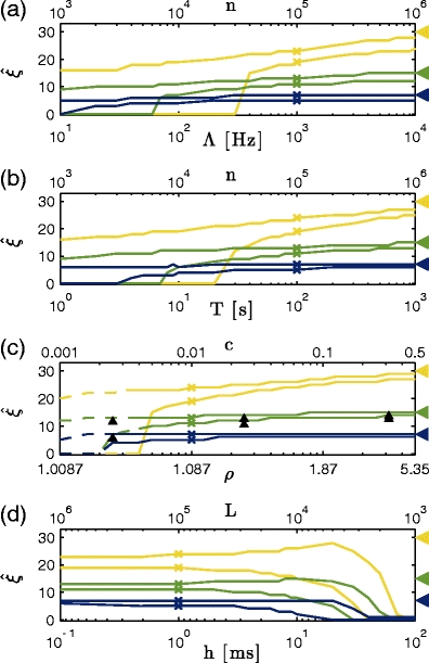
Parameter dependence of CuBIC for m = 3. Shown are the percentiles ξ ₀₅ and ξ ₉₅ (lower and upper curves of same color, respectively; see Fig. 5(b)), as a function of (a) the population firing rate Λ, (b) the duration of the experiment T, (c) the correlation strength ρ, and (d) the bin width h for data sets with correlation of maximal order ξ _syn = 7 (dark blue), ξ _syn = 15 (green) and ξ _syn = 30 (yellow). Crosses denote default parameter combinations (Λ = 10³ Hz, T = 100 s, ρ = 1.087 and h = 1 ms) one of which is varied in the different panels. Additional x axes show corresponding values of the total spike count n = ΛT (a and b), the pairwise correlation coefficient c assuming a population of N = 100 neurons, N _C = 30 of which are homogeneously correlated (c), and the sample size (d). Arrowheads on the right indicate ξ _syn, which is the optimal value for ξ ₉₅. Data points for the dashed lines in (c) contain data sets were k ₂ did not significantly exceed k ₁ (compare Section 4.2.2). Upward arrowheads in (c) denote the percentiles for the parameter combinations of Fig. 5(b)

The rejection of the null hypothesis for a given ξ implies that the pairwise correlations in the data are not compatible with the assumption that there is no correlation beyond order ξ. Thus, rejecting implies that ξ + 1 is a lower bound for the order of correlation.

Testing higher-order correlations (m > 2)

We now generalize the tests with measured pairwise correlations (m = 2) to exploit also estimated correlations of higher order (m > 2). The difference to the tests with m = 2 is that the upper bound for the mth cumulant involves all cumulants up to order m − 1. The generalization of the maximization problem (Eq. (4)) reads

8

where, as before, the κ _i[Z′] are the cumulants of the random variable Z′. Using the ν-parametrization of Eq. (5), we can rewrite Eq. (8) as the Linear Programming Problem

9

where Ξ^m − 1 is a (ξ×m − 1)-dimensional coefficient matrix with entries , and is the column-vector of the first m − 1 cumulants of Z′. Solving Eq. (9) yields both the maximal mth cumulant and the rate vector , which again can be used to compute the corresponding model parameters ν ^* and .

In direct analogy to the case m = 2, the (m,ξ)-null hypothesis states that correlation of orders 1,2,...,m are compatible with the assumption that there is no correlation beyond order ξ. This implies that κ _m[Z′] falls below the upper bound , and we define

To test a sample {Z′₁,...,Z′_L} against , we estimate correlations of order m by the mth sample cumulant of the population spike count, the so-called the mth k-statistics k _m (Stuart and Ord 1987; the sample mean and unbiased sample variance defined above are the first two k-statistics). And again, we assume that Z′ is the population spike count of the CPP model that solves Eq. (4) after the unknown κ _i[Z′] have been replaced by the estimates k _i (i = 1,...,m − 1). Then, the test statistics k _m is normally distributed with mean and variance , where expressions for can be found in the literature (Stuart and Ord 1987). The p-value of is thus given by

10

Note that after substituting the true cumulant vector by its estimate in Eq. (9), the resulting constraint consists of m − 1 equations for the ξ positive parameters ν ₁,...,ν _ξ. Unfortunately, there can be combinations of estimated cumulants for which these equations cannot be solved. In this case, Eq. (9) does not posses a solution, and the corresponding null hypothesis cannot be tested (see also Section 3.3).

Computing the lower bound

In the preceding section, CuBIC was presented as a collection of hypothesis tests , labeled by the indices m (the order of the estimated cumulant) and ξ (the maximal order of correlation in the null). We now combine these tests to infer a lower bound for the order of correlation in a given data set. To do so, recall that rejecting for given m and ξ implies that the combination of the first m cumulants requires correlation of order > ξ. As a consequence, every rejected hypothesis implies that ξ + 1 is a lower bound for the highest order of correlation in the data. The question thus is: which of these bounds should we use?

Evidently, we aim to infer the highest order of correlation that is present in the data. Hence, the objective is to find the maximum of all the lower bounds that were obtained from the hierarchy of tests. We thus aim for the pair (m,ξ) with the highest value of ξ such that the corresponding null hypothesis is rejected.

A conceptual algorithm for this search is presented in Fig. 3. It consists of two nested loops: for a fixed order of the estimated cumulant m, the inner loop searches the highest ξ for which is rejected; the outer loop iterates over subsequent orders m. The free parameters of the algorithm are the test level α, and, to ensure termination of the loops, upper bounds for the cumulant (m _max) and the maximal order of correlation assumed in the null (ξ _max; see Section 5 for their choice). After initializing the test variables (m = 2, ξ = 1, ), we estimate the first m cumulants from the data by computing the corresponding k-statistics. Next, we check if Eq. (9) is solvable for the current values of m and ξ (yellow box). This check consists of two steps. The first step checks if the first m − 1 estimated cumulants increase with order m, a requirement of the CPP model assumed to underlie the data (left rhomb in yellow box; compare last paragraph of Section 2.3). If this is not the case, then k ₁ ≤ k ₂ ≤ ... ≤ k _{m′ − 1} is false for all m′ ≥ m, which implies that Eq. (9) cannot be solved for m′ ≥ m. If the solution, i.e. the maximal cumulant and the model parameters ν ^* and , are not available, however, the corresponding p-values (Eq. (10)) cannot be computed. In this case, no hypothesis with m′ ≥ m can be tested, and the procedure is terminated. If the first m − 1 estimated cumulants are in principle compatible with the CPP, we check in the second step if the current value of ξ can solve Eq. (9) (right rhomb in yellow box). If this is not the case, ξ is increased by 1 until either Eq. (9) can be solved, or ξ reaches its upper bound ξ _max. In the former case, the data are tested against (blue box), in the latter case the test is skipped. At rejection of (rightward arrow at the box p _m,ξ < α) we set and, unless ξ reached the upper bound ξ _max, repeat the inner loop with ξ set to ξ + 1. The loop terminates with , which is the largest lower bound for the current value of m. As we reject the “zeroth” hypothesis by convention (every data set has correlations of order > 0), this holds even if the tests for the current value of m were skipped. The inner loop is repeated with new m set to m + 1, until m reaches the upper bound m _max. Finally, the lower bounds obtained for the different values of m are compared, and their maximum is returned as the absolute lower bound . A MatLab-implementation of the proposed algorithm is available upon request.

Fig. 3.

Procedure to infer the highest lower bound for the order of correlation in a given data set. The pair (m,ξ) with the highest ξ such that the corresponding null hypothesis is rejected is found by two nested loops. For any given m, the inner loop over ξ increases the lower bound , whenever Eq. (9) can be solved (right rhomb in upper yellow box) and the corresponding hypothesis is rejected (p _m,ξ < α). This loop terminates (p _m,ξ ≥ α or ξ ≤ ξ _max) with , which is the highest lower bound for the current value of m. The outer loop runs over the order of estimated cumulants m. The procedure terminates if the first m − 1 estimated cumulants violate the constraints of the CPP model (left rhomb in upper yellow box), or if the the order of the cumulant m reached the predefined upper bound m _max (rhomb below lower blue box). Finally, the bounds for different m are compared and their maximum is returned

Simulation results

Illustration

Before we present a systematic analysis of the proposed procedure in Section 4.2, we illustrate CuBIC’s sensitivity by a comparison of three sample data sets (Fig. 4). All three data sets are based on the same number of neurons (N = 100) with identical firing rates (λ = 10 Hz) and pairwise correlations (c = 0.01 in N _C = 30 and c = 0 in the remaining 70 neurons). The difference between the data sets lies solely in their higher-order correlation structure, i.e. their maximal order of correlation (Fig. 4, top panels). All sets have amplitudes at ξ = 1 that generate independent “background spikes”. Correlations are induced by additional events of amplitudes ξ _syn > 1 that differ across data sets: ξ _syn = 2 in Set1 (left), ξ _syn = 7 in Set2 (middle), and ξ _syn = 15 in Set3 (right). Thus, Set1 has correlation of order 1 and 2, Set2 has correlations up to order 7, and Set3 has correlations up to order 15. The identical pairwise correlations in the three data sets are achieved by adjusting the rate of the higher-order events (see Appendix B for the relationship between the model parameters ν,f _A and the population statistics N,N _C,λ and c). Test parameters were set to ξ _max = 15 and m _max = 4.

The similarity of the raster displays and population spike counts (Fig. 4, 2nd and 3rd from top) of the three data sets may illustrate that such standard visualization methods cannot reveal the differences in the higher-order properties of the data sets. Larger probabilities for patterns of high complexity induced by the higher-order correlations present in Set2 and Set3 are visible in the complexity distributions (third row of panels) only when plotted on a logarithmic scale (green lines). The low rates of the higher-order events imposed by the small pairwise correlations (ν ₇ = 2.07 Hz in Set2, ν ₁₅ = 0.41 Hz in Set3) makes their detection in the three distributions (bars) very difficult on a linear scale.

The identical pairwise correlations in all three data sets are reflected in identical results for tests with m = 2. For all data sets, is rejected (p < 0.05, indicated by red marks) only for ξ = 1, implying that the pairwise correlations are significant and events of amplitude 1 are not enough to explain the data. As is retained for ξ > 1 in all data sets (p > 0.05), the lower bound for m = 2 is (see Fig. 3), i.e. the tests with m = 2 do not imply correlation of order ≥ 2 in any of the data sets.

Test results with m = 3 differ strongly for the three data sets (Fig. 4, lower panels, right graphs). For Set1, only is rejected and all for ξ ≥ 2 are retained. Hence . For Set2, is rejected for ξ = 1,...,6, yielding , while for Set3 the rejection of all null-hypotheses for ξ ≤ 12 yields . In all tests with m = 4 (data not shown), the smallest values for ξ that solved Eq. (9) yielded non-significant p values (for Set1 p _4,2 = 0.5, for Set2 p _4,9 = 0.8, for Set3 p _4,16 = 0.67). Hence, no hypothesis with m = 4 was rejected except for which is rejected by convention. Thus, in all data sets. For the total lower bounds , we thus obtain for Set1, for Set2, and for Set3.

The lower bound corresponds to the maximal order of correlation in Set1 (ξ _syn = 2) and Set2 (ξ _syn = 7). Only for Set3 the lower bound falls short of the true maximum by 2 (ξ _syn = 15), but nevertheless indicates correlations of higher order than in Set2. Taken together, the three examples illustrate that CuBIC reliably detects differences in higher-order statistics, even if firing rates (here λ = 10 Hz) and very small pairwise correlations (here c = 0.01 in 30 out of 100 neurons) are identical.

Parameter dependence of test performance

Several parameters are likely to influence CuBIC’s performance. For instance, the number of recorded neurons, N, the collection of firing rates, λ ₁,...,λ _N, the duration of the experiment, T, and the bin size, h, influence the amount of available data and can thus be expected to effect test results. Also the correlation structure, i.e. the rate and the order of injected coincidences, parametrized by the N − 1 probabilities of the amplitude distribution f _A, is likely to affect the performance of the method. However, some of the parameters mentioned above are in fact redundant with respect to the test statistics used here, i.e. the k-statistics of the population spike count Z. For instance, Z depends only on the summed firing rate , but not on the precise combination of the rates of individual neurons. To analyze the parameter dependence of CuBIC (Section 4.2.3), we focus on parameters that are relevant in experimental data and avoid the above-mentioned redundancies. Furthermore, we restrict our analysis to tests with the third cumulant, thus study the inner loop in Fig. 3 for m = 3. To keep notation simple, we drop the subscript 3 and write in the remainder of this section. The upper bound for ξ was ξ _max = 30 in all simulations.

Parameters

We investigate the performance of CuBIC with respect to five parameters: the duration of the experiment, T, the total firing rate of the population, , the bin width used to discretize the data, h, and two parameters, ξ _syn and ρ, that characterize the correlation structure (amplitude distribution, f _A) of the data. We here consider amplitude distributions that consist of two isolated peaks only: a “background-peak” at ξ = 1 and a second peak at ξ = ξ _syn that determines the maximal order of correlation in the data (see for examples Fig. 4, top row). The relative height of the two peaks is parametrized by the moments ratio

11

where is the ith moment of A.

Substituting the moments μ _i[A] in Eq. (11) by the cumulants of Z via Eq. (3) shows that ρ equals the Fano Factor of the population spike count, i.e. (see e.g., Kumar et al. 2008; Kriener et al. 2008). This interpretation is valid for arbitrary amplitude distributions, and provides a method to estimate ρ from data. For a more intuitive interpretation of ρ, consider a population of N neurons with identical firing rates, where a sub-population of N _C neurons forms a homogeneously correlated subgroup, while the remaining N − N _C neurons fire independently (compare rasters displays in Fig. 4). In this case ρ relates to the (average) pairwise count correlation coefficient c of the correlated subgroup

12

For a derivation of this relation see Appendix B, Eq. (29). In case of a completely homogeneous population with N = N _C, this simplifies to (compare e.g., Kumar et al. 2008; Kriener et al. 2008). In either case, the correlation parameter ρ determines the effect of higher-order events on the pairwise correlations in the population.

Quantification of test performance

We asses CuBIC’s performance by Monte-Carlo techniques. That is, we compute the lower bound for the order of correlation (Figs. 3 and 5(a)) for each of 1000 data sets that are simulated from the CPP model with identical parameter combinations. The resulting (estimated) distribution then indicates the range of lower bounds for this particular parameter combination. We thus study the parameter dependence of CuBIC’s performance by the parameter dependence of the distribution of (Fig. 5(b)). For the specific parameter combination of Fig 5(a), for instance, lower bounds fall almost exclusively between and (Fig. 5(b), bottom panel). Increasing the correlation parameter ρ gradually sharpens and shifts to higher values of (Fig. 5(b)). CuBIC performs optimally if the lower bound corresponds to the maximal order of correlation in all Monte-Carlo simulations, i.e. if for all data sets. In this case, is a delta-peak located at ξ _syn (Fig. 5(b), top panel).

Fig. 5.

Quantification of test performance. (a) p-values for tests against and the resulting lower bound for the order of correlation (here ) for one data set (parameters: ξ _syn = 15, Λ = 10³ Hz, T = 100 s, ρ = 1.02 and h = 1 ms). Red filled circles denote rejected hypotheses, i.e. p-values below 0.05. (b) Three estimated distributions of lower bounds , each obtained via Monte-Carlo simulations of 1000 data sets with identical parameter combinations. Parameters as in (a), only for different values of the correlation parameter (bottom: ρ = 1.02, middle: ρ = 1.2; top: ρ = 3.75). The two percentiles and are marked by arrowheads (see text for interpretation), also at the corresponding parameter values in Fig. 6(c). Observe the shift and sharpening of towards the maximal order of correlation in the data ξ _syn = 15 (dashed line) for increasing ρ

To further reduce complexity, we will discuss the parameter dependence of by means of the two percentiles (black triangles in Fig. 5(b))

CuBIC performs optimally if is a delta peak as in Fig. 5(b), top panel, i.e. if ξ ₀₅ + 1 = ξ _syn = ξ ₉₅. More generally, a value of ξ ₀₅ ≫ 0 indicates that CuBIC reliably infers the existence of higher-order correlations ( in 95% of all cases), while a value of ξ ₉₅ ≤ ξ _syn guarantees that the actual order is not overestimated ( in less than 5% of all cases, no false positives).

As mentioned before (Section 3.3), certain combinations of sample cumulants, e.g. k ₂ < k ₁, represent untestable data sets and yield lower bounds of . To avoid border effects for extremely small pairwise correlations (ρ < 1.05), we set not only if k ₂ < k ₁ but also if k ₂ does not significantly exceed k ₁, i.e. if is retained (marked as dotted lines in Fig 6(c)).

Results

Figure 6 shows the dependence of CuBIC’s performance on the population firing rate Λ (Fig. 6(a)), the duration of the experiment T (Fig. 6(b)), the correlation strength (population Fano Factor) ρ (Fig. 6(c)) and the bin width h (Fig. 6(d)) for different values of ξ _syn (crosses in Fig. 6(a–d) denote the default parameters that are fixed while only one of them is varied).

Changes in the population firing rate Λ, the duration of the experiment T, and the correlation strength ρ have qualitatively very similar effects on the performance (Fig. 6(a), (b), and (c), respectively). For all analyzed values of ξ _syn (dark blue, green, and yellow lines) and small values of either of the parameters, i.e. Λ = 10 Hz (Fig. 6(a)), T = 1 s (Fig. 6(b)) or ρ = 1.0087 (Fig. 6(c)), the distributions of lower bounds extend from ξ ₀₅ = 0 (lower lines) to ξ ₉₅ < ξ _syn (upper lines below colored triangles). Hence, lower bounds might not exceed the trivial value of for such small parameter values. Increasing either of the parameters gradually shifts , i.e. ξ ₀₅ and ξ ₉₅, to higher values of , thus indicating improved performance. The exact quality of the performance, captured by the width of , i.e. the distance between ξ ₀₅ and ξ ₉₅, and in particular its difference from ξ _syn (colored triangles, compare also Fig. 5(b)), depends crucially on the order of correlation ξ _syn present in the data.

For ξ _syn = 7 (dark blue lines), CuBIC performs optimally (ξ ₀₅ + 1 = 7 = ξ ₉₅, compare Fig. 5(b)) for experiment durations of T > 100 s (Fig. 6(b)) and a wide range population Fano Factors (ρ ≥ 1.17, Fig. 6(c)). Such optimality is not guaranteed for the analyzed range of the population firing rate Λ, although population rates above Λ = 400 Hz yield a lower percentile of ξ ₀₅ = 5, indicating close-to-optimal performance ( in 95% of all cases, Fig. 6(a)). Smaller values of either of the parameters shift to lower values, indicating impaired performance. Nevertheless, as the lower percentile ξ ₀₅ is considerably larger than zero even for population rates as low as Λ = 20 Hz, experiment durations of T = 6 s and population Fano Factors of ρ = 1.02, CuBIC reliably detects the presence of higher-order correlations for a wide range of parameter combinations.

In the other extreme, where the same pairwise correlations (identical value of ρ) are realized by correlations of order ξ _syn = 30 (yellow lines), falls short of its optimum (ξ ₀₅ + 1 = 30 = ξ ₉₅, see Fig. 5(b), top panel) even for high values of all investigated parameters, i.e. population rates of Λ = 10⁴ Hz, experiment durations of T = 10³ s and correlation strengths of ρ = 5.35 (Fig. 6(a), (b) and (c), respectively). Note, however, that also here ξ ₀₅ ≫ 0 even for moderate values of Λ, T and ρ, implying that the presence of higher-order correlations is reliably detected, albeit not their actual order. For the default values Λ = 10³ Hz, T = 100 s and ρ = 1.087 (yellow crosses in Fig. 6(a–d)), for instance, lower bounds for ξ _syn = 30 fall between and in 90% of the analyzed data sets (ξ ₀₅ = 19, ξ ₉₅ = 24).

Test performance for ξ _syn = 15 (green lines) is somewhere in between the often optimal results for ξ _syn = 7 and the more indicative results for ξ _syn = 30. In short, optimal performance is achieved only for high population Fano Factors (ρ ≥ 3.75, rightmost black triangle in Fig. 6(c)), while the presence of higher-order correlations is reliably detected () for a wide range of parameters (Λ > 70 Hz, Fig. 6(a), T ≥ 80 s, Fig. 6(b), and ρ ≥ 1.02 Hz, Fig. 6(c)).

The qualitative similarity between Fig. 6(a) and (b) result from the identical effect of the varied parameters, Λ and T, on the expected spike count n = ΛT (Fig. 6(a), (b), top x axis). As n affects the quality of the estimators k _i , both Λ and T influence test results in a similar manner. The similar ρ-dependence results from the fact that increasing ρ increases the probability for high-amplitude events f _A(ξ _syn), which simplifies their detection (Fig. 6(c)).

Changes in the bin width h (Fig. 6(d)) affect CuBIC’s performance for all values of ξ _syn in a very similar way. Increasing h decreases the lower percentile from ξ ₀₅ ≫ 0 at h = 0.1 ms to ξ ₀₅ = 0 for h = 100 ms, irrespective of ξ _syn. The upper percentiles ξ ₉₅ (upper lines) can even show non-monotonic behavior: for ξ _syn = 15 (green) and ξ _syn = 30 (yellow), ξ ₉₅ increases for values between 1 ≤ h ≤ 60 ms and decreases for h > 60 ms. The median of , which lies roughly in the middle of ξ ₀₅ and ξ ₉₅, however, remains approximately constant for h ≤ 60 ms, at least for ξ _syn = 15 and ξ _syn = 30 (green and yellow, respectively). Therefore, the average lower bound remains approximately constant as long as h ≤ 10 (L ≥ 10⁴, top axis), but only the variability of , i.e. the distance between ξ ₀₅ and ξ ₉₅, increases for this range of h.

We wish to stress that the larger variability of for increased bin sizes is not so much due to the increased average spike count per bin μ = Λh, but rather the resulting decreased sample size (Fig. 6(d), top x-axis). The expected spike count μ = Λh changes with the population rate Λ and the bin width h in the exact same manner. However, while increasing μ via Λ (Fig. 6(a)) from the default value Λ = 10³ Hz (crosses) to Λ = 10⁴ Hz does not alter test performance for ξ _syn = 7 (dark blue lines), increasing μ via the bin width from h = 1 ms to h = 10 ms (Fig. 6(d)) drastically reduces the lower percentile ξ ₀₅ (lower dark blue line in Fig. 6(d)). The decrease in sample size increases the variance of our test statistic (compare Eq. (7)) and therefore decreases test power.

Summary of results

The simulation results of the previous section show that CuBIC reliably detects the presence of higher-order correlations for a wide range of parameter values. As CuBIC is not designed to directly estimate the order of correlation, the inferred lower bound might not always correspond to the maximal order of correlation present in a given data set. The most important parameter is the sample size L, which is required to be ≥ 10⁴ to reliably detect higher-order correlations (Fig. 6(d)), corresponding to e.g. an experiment of T = 50 s duration analyzed with a bin size of h = 5 ms. Furthermore, total spike counts of n = 10⁴ (e.g. N = 100 neurons firing at 1 Hz for T = 100 s; Fig. 6(a) and (b)) and a correlation parameter (population Fano Factor) in the order of ρ = 1.087 suffice for the test to reliably detect the presence of higher-order correlations (lower percentiles ξ ₀₅ > 0, green and dark blue lower lines Fig. 6(a–c)) if correlations in the data are of moderate order (ξ _syn = 7 and ξ _syn = 15, green and dark blue lines).

Discussion

The identification of active cell-assemblies in simultaneously recorded spike trains has been the topic of extensive research (Gerstein et al. 1985, 1989; Sakurai 1998; Martignon et al. 2000; Grün et al. 2002a, b; Harris 2005; Schrader et al. 2008). Analysis tools that go beyond pairs of neurons, however, face severe limitations due to limited sample sizes of typical electrophysiological recordings (Martignon et al. 1995, 2000; Brown et al. 2004). The cumulant based inference of higher-order correlations (CuBIC) presented in this study avoids the need for extensive sample sizes. This is achieved by a combination of three ingredients: (1) pooling, i.e. using the population spike count and its cumulants to measure correlations in the population; (2) using the compound Poisson process (CPP) as a parametric model for correlated spiking populations; and (3) exploiting the constraining relations among correlations of lower and higher order in large neuronal pools.

Initially, we presented CuBIC as a hierarchy of hypothesis tests , indexed by the order of the estimated cumulants m and the maximal order of correlation ξ allowed in the null. The algorithm of Fig. 3 combines these tests to infer a lower bound on the order of correlation in a given data set (see also Section 3.3). As free parameters, the algorithm requires upper bounds for m (m _max) and ξ (ξ _max) to be chosen by the experimenter. To chose m _max, recall that CuBIC is extremely sensitive for higher-order correlations already with m = 3 (Fig. 6). For the parameters analyzed here, tests with m = 4 increased only occasionally, as the smallest ξ that solved Eq. (9) typically yielded non-significant p-values (data not shown). Furthermore, the reliable estimation of high cumulants is known to require vast sample sizes. Therefore, although tests with m > 3 can in principle yield additional information, we do not expect that choosing the bound for m larger m _max = 4 improves test results in situations with sample sizes compatible with electrophysiological experiments. To chose the upper bound for ξ, note that ξ _max is also an upper bound for . As the maximal order of correlation in the data has to be smaller than the number of recorded neurons N, we know that must hold. This suggests to chose ξ _max = N, as higher values of ξ _max cannot increase . If the analysis was based on multi-unit activity and the number of recorded neurons is unknown, an a posteriori criterion on whether the chosen value for ξ _max was high enough can be obtained by inspecting tests with ξ = ξ _max. That is, if was rejected for some m, hypothesis with ξ > ξ _max might also have been rejected, potentially resulting in higher . Thus, if tests against are retained for all m, the chosen ξ _max was high enough.

The procedure was calibrated with rather restricted model classes, namely amplitude distributions with two isolated peaks. Thus, the question arises how differences in the correlation structure would influence CuBICs performance. In the numerical examples of this study, CuBIC used only the first three cumulants of the data, which depend on the first three moments of the amplitude distribution (compare Eq. (3)). As a consequence, if the data under consideration had a different amplitude distribution, however with similar first three moments, CuBIC will produce similar results. If, for instance, the additional isolated peak at ξ _syn is exchanged by a somewhat distributed peak centered at ξ _syn, the inferred lower bound will be similar.

Importantly, CuBIC is not designed to directly estimate the “true” maximal order of correlation in the data. Furthermore, the neuron IDs that realize the correlations are currently not resolved. It is important to keep in mind, however, that approaches that pose such specific question to the data face severe limitations with respect to the size of the analyzed populations (e.g., Shlens et al. 2006; see also Section 5.1). Thus, we regard the less specific lower bound obtained by CuBIC as the price to pay when analyzing large populations. Renouncing the specific questions is precisely what allows CuBIC to detect higher-order correlations in data sets with previously unreached population size (N∼100) and sample sizes compatible with physiological experiments (see Figs. 4 and 6).

Model dependence of higher-order correlations

The role of correlations for cortical information processing has been lively debated (Abeles 1991; Shadlen and Newsome 1994; Riehle et al. 1997; Singer 1999; Abbott and Dayan 1999; Kohn and Smith 2005; Schneidman et al. 2006; Shlens et al. 2006; Laurent 2006; Pillow et al. 2008). While in the meantime pairwise correlations are widely accepted as a relevant feature of parallel spike trains, the relevance of higher-order correlations is controversial. In fact, several recent studies raised doubts about the importance of higher-order interactions. In two studies that explore multi-neuron firing patterns in primate (Shlens et al. 2006) and salamander (Schneidman et al. 2006) retina, data were collected for fairly long times (∼1 hour), and distributions of the binary patterns P _N for sub-populations with N ≤ 10 were estimated. Based on this, a surrogate distribution was generated that reproduces the pairwise correlations in the population, but disregards all higher-order parameters: the “maximum entropy distribution” P ₂. A comparison of P _N with P ₂ provides estimates on the amount of information contained in the higher-order parameters. The results of both studies indicate that only a negligible fraction of the total information is contained in the higher-order parameters (less than 2% in primate retina according to Shlens et al. 2006, and less than 10% in salamander retina according to Schneidman et al. 2006), and a recent study reports similar values for neo-cortical networks (Tang et al. 2008). In other words: almost the entire information available in the distribution of multi-neuron firing patterns can already be inferred from pairwise correlations. So why bother estimating higher-order parameters?

The consequences of the maximum entropy results for the relevance of CuBIC are difficult to judge. First of all, the maximum entropy approach does not appear to be very sensitive for higher-order correlations. As shown by Shlens et al. (2006), additional higher-order coincidences with a rate of ∼0.3Hz among the N = 7 analyzed neurons would not have altered their results. This “coincidence rate”, however, lies in the parameter range of Set3 of Fig. 4 (here ν ₁₅ = 0.41Hz). In this range CuBIC detected correlations of order ≥ 13, illustrating the comparatively low sensitivity of the maximum entropy approach for existing higher-order correlations. Second, the combinatorial explosion of the parameter space limits maximum entropy approaches to only relatively small populations (), unless additional assumptions are imposed on the data (Montani et al. 2009; Shlens et al. 2009). Theoretical evidence suggests, however, that the relevance of higher-order correlations increases with the size of the neuronal population (Roudi et al. 2009). In fact, using N = 24 unsorted multi-unit spike trains of the rodent whisker system, Montani et al. (2009) report a significant increase in information if additional to the pairwise interactions also triplet interactions are taken into account. Taken together, we firmly believe that the analysis of large groups with methods that are sensitive to higher-order correlations is inevitable to uncover their role in cortical computation.

Our third remark concerns the conceptual differences between cumulant correlation as measured here, and the higher-order parameters used in the maximum entropy framework. The latter is based on the prominent binary exponential family (Martignon et al. 1995; Nakahara and Amari 2002; Martignon et al. 2000; Gütig et al. 2003; Del Prete et al. 2004; Shimazaki et al. 2009). In this setting, spike trains are represented as binary sequences, such that X _i(s) = 1 if the ith neuron has one or more spikes in the sth bin, and X _i(s) = 0 otherwise. Assuming stationarity and no memory, the multivariate distribution function of the binary pattern vector X admits the representation

In this framework, higher-order correlations are reflected in nonzero “higher-order parameters” θ. For example, θ _ijk quantifies third-order interactions of the triplet (X _i,X _j,X _k). Importantly, these higher-order parameters are neither equivalent, nor related in any straightforward way to the cumulant correlations employed by CuBIC (see Section 2.1.1 and Appendix A). A major difference, for instance, results from the equivalence of cumulant-based correlations with the concept of coincident events addressed by the CPP (Theorem 1). Given that these coincidences are perfectly synchronized, changes in the bin width h do not affect cumulant-based correlations. In contrast, as changes in the bin width alter the shape of p _X, the interaction parameters θ inevitably change with h. Observe that the bin size dependence of θ does not result from the fact that larger bins measure correlations on a broader time scale as the time scale of correlation was assumed to be instantaneous, but is rather inherent to the exponential family. More generally, cumulant correlations determine to what extent expectation values of products factorize (e.g., Stratonovich 1967, and our Section 2.1.1), while the higher-order parameters in the exponential family measure to what extent the probability of certain binary patterns can be explained by the probabilities of its sub-patterns (e.g., Gütig et al. 2003). Taken together, the two frameworks are designed for different purposes, and can hence be expected to be sensitive to different features of the data. A better insight into their relationship presents an important path for future research (see also Staude et al. 2010, for a more detailed discussion).

Our main motivation to use cumulant correlations is that they enable us to analyze large populations of simultaneously recorded spike trains. As opposed to the θ parameters, cumulant correlations can be inferred from the population spike count Z,. Thereby, the multivariate problem to estimate correlations for all 2^N − 1 subgroups is transferred into a parsimoniously parametrized univariate problem with N parameters. The small sample size required by CuBIC and its ability to analyze populations of N > 100 neurons is a direct consequence of this property. Furthermore, the compound Poisson process presents a very intuitive interpretation of cumulant correlations (Theorem 1) that directly implements the concept of temporally coordinated spikes (see also Staude et al. 2008). And finally, the exponential family captures imprecise correlations only at the cost of ignoring spikes by clipping, as it requires the variables X _i to be binary (e.g., Del Prete et al. 2004), whereas cumulant correlations can be measured among arbitrary spike counts. We conclude that the adequate framework to analyze a given data set should be carefully chosen in view of the specific scientific question. For the detection of temporally coordinated spikes in large neuronal populations, we believe that cumulant-based correlations as exploited by CuBIC are well-suited.

Relation to other tools

While algorithms for the generation of correlated spike trains are becoming available (e.g., Kuhn et al. 2003; Niebur 2007; Staude et al. 2008; Brette 2009; Macke et al. 2008; Krumin and Shoham 2009), only few of these models can be exploited for data analysis. In an approach similar to ours, Ehm et al. (2007) derive estimators of the continuous time parameters (analogous to our carrier rate and amplitude distribution) from the Poissonized bin counts (here: “population spike count”) via Fourier inversion of the empirical characteristic function. Instead of inferring lower bounds as in CuBIC, “empirical de-Poissonization” presented by Ehm et al. (2007) thus directly estimates the orders of correlation in the data. However, the more explicit parameters appear to impose constraints on the data, such that particular care is required if the expected number of spikes per bin exceeds a critical value. A comparison of CuBIC and the empirical de-Poissonization to resolve their respective advantages and disadvantages is currently under way (Reimer et al. 2009).

Besides the higher-order approaches described above, the majority of available analysis tools for massively parallel spike trains either exploit pairwise statistics to infer inter-correlated groups by using some sort of clustering (Gerstein and Aertsen 1985; Gerstein et al. 1985; Berger et al. 2007; Grün et al. 2008b; Fujisawa et al. 2008), or test the occurrence of specific patterns against the assumption of complete (Grün et al. 2002a; Pipa et al. 2008) or partial independence (Berger et al. 2010). The three examples depicted in Fig. (4), however, illustrate the limitations of both approaches. First, the three data sets have identical second order statistics, making it impossible for pairwise approaches to differentiate between them. Second, the combinatorial explosion prevents the analysis of populations sizes of N~100 neurons with pattern-based approaches. And third, it is unclear whether either approach is sensitive enough to detect correlated groups when pairwise correlation are as low as discussed here.

A novel approach that is recently gaining attention starts from the analytically tractable generalized linear model (GLM), and estimates its parameters by maximum likelihood techniques (Paninski 2004; Truccolo et al. 2005; Okatan et al. 2005; Pillow et al. 2008). The power of this framework is that estimated parameters can be interpreted in terms of network properties like e.g. synaptic interactions between nerve cells, stimulus-response properties and the history dependence of individual spike trains. To understand how such anatomical and biophysical attributes of neuronal populations relate to higher-order correlations in the joint spiking of groups of neurons as detected by CuBIC is subject of current research.

Constraining relations among correlations of different order have also been studied by Amari et al. (2003), Johnson and Goodman (unpublished manuscript) and Benucci et al. (2004). The latter study defined a combinatorial algorithm to obtain upper bounds for certain observables. Closer to our approach is the study of Johnson and Goodman (unpublished manuscript), who derive explicit constraints among correlation coefficients of different orders within the CPP framework. However, both studies do not provide confidence intervals, hence are not applicable to data analysis in a straightforward way. Amari et al. (2003) investigated the relation between population variance and higher-order correlations in the information geometric framework (Amari and Nagaoka 2000) for the limit of large population sizes (N→ ∞). The result is similar to our findings in the sense that a high population variance implies higher-order correlations. However, results from large N provide only qualitative suggestions for data analysis.

Consequences of underlying model

An important ingredient of the present study is to use the CPP as a model for correlated spike trains. A consequence of this model-driven approach is that the reliability of obtained test results depends crucially on how well the CPP is suited to describe populations of spiking neurons in general, and assembly activity in particular.

Stationarity

We presented the CPP as a model of a stationary population, i.e. where individual spike trains have constant firing rates. However, cortical spike trains typically undergo both stimulus-driven and internally generated changes in firing rate. To analyze also such non-stationary data sets, the relatively small required sample size enables us to use a “sliding-window” approach (see e.g., Grün et al. 2002b), where data are cut into quasi-stationary windows of e.g. 100 ms and the statistics is therein obtained over trials. For the case of 100 trials analyzed with a bin width of h = 1 ms, this would yield L = 10⁴ samples, which is perfectly in the required range for CuBIC to yield lower bounds close to the actual order of correlation (compare Fig. 6(d)). An alternative could be to directly include the non-stationarities in the model (Staude and Rotter 2009). Both approaches present important aspects of future research.

Single-process properties

Recent studies of cortical spike trains criticize the use of Poisson processes as models for single spike trains (Amarasingham et al. 2006; Nawrot et al. 2008). Without doubt, inclusion of process types deviating from Poisson in the generating model presents a major challenge for the presented procedure. However, criticism against the Poisson model for cortical spike trains is typically motivated by either non-exponential interval statistics (e.g., Maimon and Assad 2009), or non-Poissonian spike count distributions for large bin sizes (h > 50 ms) and high firing rates under ’optimal’ stimulation (λ > 50 Hz; e.g. Amarasingham et al. 2006). Both of these aspects are of little impact if the counting statistics is sampled with small (h ≤ 10 ms) bin sizes. In such a scenario, and in particular for low firing rates (e.g. Lennie 2003; Lee et al. 2006; Olshausen and Field 2006; Maldonado et al. 2008), neurons will have at most one spike per bin, leading to almost identical counting statistics for Poisson processes and other process types (e.g. gamma processes; van Vreeswijk 2006; Nawrot et al. 2008). Note also that the CPP does not directly model individual processes as Poisson processes, but only assumes the carrier processes to be Poisson. Importantly, the latter can be a good approximation even if individual processes deviate from strict Poisson statistics. For instance, if background spikes are Poisson and high-amplitude events are very regular but have a very low rate (as in Fig. 4), the carrier process is still well approximated by a Poisson process. More generally, the sum of increasingly sparse point processes converge to a Poisson process (Daley and Vere-Jones 2005, but see Lindner 2006; Câteau and Reyes 2006). Although these aspects need to be considered and will be subject of further research, we therefore expect CuBIC to yield reliable results even if single processes deviate from the Poisson assumption (Staude et al. 2007).

Precision of coincidences

Cortical correlations are reported on a variety of time scales, from precise correlations within a few few ms (Grün et al. 1999; Kohn and Smith 2005; Pazienti et al. 2008; Desbordes et al. 2008) to slow covariations of firing rates on a time scale of > 50ms (e.g., Kohn and Smith 2005; Smith and Kohn 2008). The perfect temporal precision of the joint spikes generated by the CPP may thus be questioned as a biologically plausible model of experimental spike trains. In the present study, the CPP was not intended to realistically model spike trains in continuous time, however. We presented the CPP strictly to interpret the correlated counting variables X _i, obtained with a given bin width h. Allowing a temporal jitter in the synchronous events, e.g. by jittering the coincident events during the inserting process (see e.g. Staude et al. 2008; Brette 2009), results in comparable counting variables X _i if this jitter is small compared to the applied bin size (Pazienti et al. 2008). Although its sensitivity for such imprecise coincidences remains to be assessed systematically, we expect CuBIC to tolerate imprecise coincidences with small but realistic jitter.

A somewhat different issue is the detection of correlations with systematic temporal offset, e.g. due to functional or “effective” connectivity (Aertsen et al. 1989; Fujisawa et al. 2008). As an extension of CuBIC to detect also non-zero-lag higher-order correlations, one may shift individual spike trains against each other and then analyze this shifted population (cmp. Grün et al. 1999). As tests for different shifts will generally not be independent, however, appropriate corrections that account for multiple testing have to be applied. Furthermore, the combinatorial explosion that emerges from shifting all spike train against each other with different delays requires smart algorithms to reduce the resulting computational cost.

Positivity of the correlations

A limitation of the CPP is that the insertion of synchronous spike events models spike coordination, not spike avoidance. As a consequence, correlations in the CPP can only be positive (Staude et al. 2008; Brette 2009). The CPP cannot model negatively correlated spike counts, that is, troughs in the cross-correlation function. Whether or not this is relevant for CuBICs applicability depends crucially on the properties of electrophysiological data. The rare reports of negative correlations, especially among cortical spike trains (e.g., Nevet et al. 2007), however, makes us confident that this is not an important limitation.

Conclusions

Based on Hebb’s original ideas (Hebb 1949), the coordinated spiking of large neuronal groups is the conceptual foundation of various “brain theories” (e.g., Eggermont 1990; Abeles 1991). However, limitations of available analysis tools has rendered the exploitation of the increasing number of simultaneously observable neurons extremely difficult. The CuBIC method presented in this study is a novel procedure to detect higher-order correlations in massively parallel spike trains, which overcomes these limitations. In particular, the sample size required by our method lies in a range that is compatible with electrophysiological experiments. CuBIC assumes data to be stationary and single processes the sum of which is appropriately modeled by the CPP, and its extension to account for dynamically changing, non-Poissonian data is the most important aspect of future work. Taken together, we regard CuBIC as a unique opportunity to analyze large populations of neurons for coordinated spike timing.

Appendix

A Higher-order correlations and the CPP

A pair of random variables X ₁ and X ₂ is uncorrelated, if the expectation of their product factorizes

and the covariance measures the degree of correlation between them. As the covariance is bounded by the square root of the individual variances, one quantifies pairwise correlations by the dimensionless correlation coefficient

13

Cumulant-correlations are a generalization of the (co-)variance to measure correlations among more than two r.v.s (e.g., Stratonovich 1967; Stuart and Ord 1987; Streitberg 1990; Papoulis and Pillai 2002; Gardiner 2003; Staude et al. 2010). The cumulants κ _m[Z] (m ∈ ℕ) of a r.v. Z are defined in terms of the coefficients of the power series expansion of the logarithm of its characteristic function

14

where Θ_Z(u) is called the “cumulant generating function” (c.g.f.) of Z. To relate the cumulants to the more familiar (raw) moments , recall that the latter are defined in terms of the coefficients of the power series expansion of the characteristic function

15

Expressions relating cumulants to moments are obtained by writing the logarithm of the right hand side of Eq. (15) as a power series in u, and collecting the coefficients. For the first two cumulants, this yields

Similar expressions for higher m are increasingly complicated, but algorithms for their computation are available (e.g. Stuart and Ord 1987; Di Nardo et al. 2008).

Given two independent r.v.s X ₁ and X ₂, we have

Writing the c.g.f.s as power series and comparing coefficients yields the central property of cumulants: the cumulant of the sum of independent random variables is the sum of the individual cumulants

If X ₁ and X ₂ are not independent, the cumulants of X ₁ + X ₂ contain also “mixed”, or “connected” cumulants. For m = 2, we obtain the well-known equation

16

17

Equation (16) implies that the second cumulant of X ₁ + X ₂ is additive-linear, if and only if , i.e. if X ₁ and X ₂ are uncorrelated. Higher-order cumulant correlations generalize the covariance in exactly this sense: they determine the “degree of linearity” of the higher cumulants (e.g., Stratonovich 1967; Gardiner 2003). Formally, higher-order cumulants arise as coefficients of the c.g.f. of vector-valued variables X = (X ₁,...,X _N)

18

19

Higher-order cumulant correlations exist, if the corresponding mixed cumulant κ _J[X] is non-zero. To be precise,

Definition 1

Let X be a random vector. Denote the number of non-zero elements of a multi-index by n _J. Then the components of X are said to have correlations of order m if there exists J ∈ ℕ^N with n _J = m such that the corresponding mixed cumulant is non-zero, i.e. κ _J[X] ≠ 0.

For multi-indices J with only one non-zero element, e.g. J = (2,0,0...,0), the mixed cumulants κ _J in Eq. (18) are simply the univariate cumulants of Eq. (14): . Furthermore, a generalization of is that mixed cumulants with identical arguments are the univariate cumulants of the appropriate order

20

Evidently, the c.g.f. of a sum of r.v.s is the multivariate c.g.f. with all arguments set to u

Inserting into Eq. (18) and comparing coefficients with Eq. (14) yields

showing in particular that the mth cumulant of Z depends on correlations of maximal order m.

Proof of Theorem 1

To prove Theorem 1 of Section 2.4, we present a multivariate version of the compound Poisson process (CPP) defined in Section 2.2 (compare Ehm et al. 2007; Staude et al. 2010). Consider N neurons {x _i(t)}_i ≤ N and let be the set of all nonempty subsets of {1,...,N}. For each , we assign a stationary Poisson process y′_M(t) with rate ν′_M that determines the points in time where the neurons {x _i(t)}_i ∈ M have a joint spike event.

Assuming all the y′_M(t)s to be independent, it is straightforward to verify that is a CPP as defined in Section 2.2, where |M| denotes the number of elements of M. The processes y _l(t) of Section 2.3 are given by y _l(t) = ∑ _|M| = l y′_M(t), and we obtain the parameters of z(t) (carrier rate ν and amplitude distribution f _A) by and . Evidently, f _A assigns non-zero probabilities to events of amplitude ≥ m if and only if at least one of the rates ν′_M with |M| ≥ m is positive. Using the above definition, Theorem 1 is thus equivalent to the equivalence of the following two statements:

1. at least one mth order mixed cumulant is non-zero, i.e. there exists a multi-index J ∈ ℕ^N with n _J ≥ m such that κ _J[X] ≠ 0

2. at least one of the processes y′_M(t) that determines coincidences of at least m of the spike trains x _i(t) has non-zero rate, i.e. there exists with |M| ≥ m and ν′_M > 0

The proof is not difficult, yet notationally cumbersome for arbitrary N. The idea is to decompose Z into the counting variables Y′_M of the y _M′(t) and show that their mixed cumulants κ _J[Y′_M] vanish if J has more non-zero elements than the multi-index associated to M.

With the variables Y′_M, the argument of κ _J[X], the pattern vector X = (X ₁,...,,X _N), can be written as

21

where is the binary vector whose ith component is 1 if i ∈ M and 0 otherwise. For given J ∈ ℕ^N, we thus have

22

where the second equality follows from the independence of the Y′_Ms. Clearly κ _J[δ _M·Y′_M] = 0 for all M with n _J > |M|, as in this case the order of the measured correlation n _J exceeds the number of non-zero components of the argument. In fact, κ _J[δ _M·Y′_M] ≠ 0 if and only if supp(J) ⊂ M, as these are the cases where we do not correlate with the variable 0 (the support supp(J) is the set of non-zero elements of J). In this case, κ _J[δ _M·Y′_M] is a cumulant of the Poisson variable Y′_M which satisfies (Eq. (20)). Hence,

This implies

23

Now we can prove the equivalence of statements (a) and (b).

“(a)⇒(b)”: Let J ⁺ ∈ ℕ^N be such that and . Then by Eq. (23), , and as all ν′_M ≥ 0 there must be at least one with supp(J) ⊂ M ⁺ and . As , this M ⁺ must have at least m elements, hence |M ⁺| ≥ m.

“(b)⇒(a)”: Let with |M ⁺| ≥ m and and let J ⁺ be the associated multi-index. Then and

□

B Model parameters and population statistics

This appendix relates the parameters of the compound Poisson process, i.e. the carrier rate ν and the amplitude distribution f _A, to parameters used in the context of physiological data, i.e. firing rates λ and pairwise count correlation coefficients c, for a population of N neurons.

Firing rates

To compute the average rate λ, observe that . With Eq. (3), we thus have

24

Pairwise Correlations

To compute the count correlation coefficient c for a fixed bin width h (Eq. (13)), recall that by definition of the variance

Denoting the population average variance and covariance by

the population Fano-Factor reads

The Poisson property of the individual processes implies , which yields . Using the identity of the population Fano-Factor with the moments ratio , we finally obtain

25

Note that by Eq. (25), the pairwise correlations, contained in r, do not depend on the details of the amplitude distribution f _A, but are completely determined by the ratio of its first two moments ρ.

If the population is homogeneous (all neurons have the same firing rate, all pairs are equally correlated, and so on), the average quantities v and r are the actual variance and covariance of the processes. In this case, the count correlation coefficient is given by , which implies

26

Conversely, the moments ratio is given by

27

Correlated subgroups

Now consider the case where N _C of the N neurons form a homogeneously correlated subgroup while the remaining N _I = N − N _C neurons are independent (see rasters in Fig. 4 for examples). In this case, we can decompose Z into the contribution of the correlated, Z _C, and the uncorrelated, Z _I, sub-populations: Z = Z _C + Z _I. Now and . We can thus write

Dividing by yields

28

For a homogeneous population as the correlated subgroup, the Fano Factor is related to the pairwise correlation coefficient via Eq. (27), i.e. . Inserting into Eq. (28) and solving for c yields the correlation coefficient of the correlated subgroup

29

Single interaction process

The amplitude distributions used in Section 4 consist of two isolated peaks

30

where δ _i,k is the Kronecker-Delta. The “single interaction process” (Kuhn et al. 2003) is the special case with ξ _in = N. Because f _A(1) + f _A(ξ _syn) = 1, this model has three free parameters ν, f _A(1) and ξ _syn, which are related to N, λ and ρ (or c) by Eqs. (24) and (29). Straightforward computation yields that homogeneous populations with mean firing rate λ and correlation parameter ρ are achieved by setting

and

Given λ and ρ are constrained, the event amplitude ξ _syn that realizes the correlation can be freely chosen as long as ν > 0 and η ∈ [0,1]. This is guaranteed if

References

- Abbott LF, Dayan P. The effect of correlated variability on the accuracy of a population code. Neural Computation. 1999;11:91–101. doi: 10.1162/089976699300016827. [DOI] [PubMed] [Google Scholar]
- Abeles M. Role of cortical neuron: Integrator or coincidence detector? Israel Joural of Medical Sciences. 1982;18:83–92. [PubMed] [Google Scholar]
- Abeles M. Corticonics: Neural circuits of the cerebral cortex. 1. Cambridge: Cambridge University Press; 1991. [Google Scholar]
- Aertsen A, Gerstein G, Habib M, Palm G. Dynamics of neuronal firing correlation: Modulation of “effective connectivity”. Journal of Neurophysiology. 1989;61(5):900–917. doi: 10.1152/jn.1989.61.5.900. [DOI] [PubMed] [Google Scholar]
- Amarasingham A, Chen T-L, Harrison MT, Sheinberg DL. Spike count reliability and the poisson hypothesis. Journal of Neuroscience. 2006;26(4):801–809. doi: 10.1523/JNEUROSCI.2948-05.2006. [DOI] [PMC free article] [PubMed] [Google Scholar]
- Amari S-i, Nagaoka H. Information geometry. New York: MS and Oxford University Press; 2000. [Google Scholar]
- Amari S-i, Nakahara H, Wu S, Sakai Y. Synchronous firing and higher-order interactions in neuron pool. Neural Computation. 2003;15:127–142. doi: 10.1162/089976603321043720. [DOI] [PubMed] [Google Scholar]
- Benucci, A., Verschure, P. F. M. J., & König, P. (2004). High-order events in cortical networks: A lower bound. Physical Review E, 70(051909). [DOI] [PubMed]
- Berger, D., Borgelt, C., Louis, S., Morrison, A., & Grün, S. (2010). Efficient identification of assembly neurons within massively parallel spike trains. Computational Intelligence and Neuroscience, 21. doi:10.1155/2010/439648. [DOI] [PMC free article] [PubMed]
- Berger D, Warren D, Normann R, Arieli A, Grün S. Spatially organized spike correlation in cat visual cortex. Neurocomputing. 2007;70(10–12):2112–2116. doi: 10.1016/j.neucom.2006.10.141. [DOI] [Google Scholar]
- Bohte SM, Spekreijse H, Roelfsema PR. The effects of pair-wise and higher-order correlations on the firing rate of a postsynaptic neuron. Neural Computation. 2000;12:153–179. doi: 10.1162/089976600300015934. [DOI] [PubMed] [Google Scholar]
- Brette R. Generation of correlated spike trains. Neural Computation. 2009;21:188–215. doi: 10.1162/neco.2009.12-07-657. [DOI] [PubMed] [Google Scholar]
- Brown EN, Kaas RE, Mitra PP. Multiple neural spike train data analysis: State-of-the-art and future challenges. Nature Neuroscience. 2004;7(5):456–461. doi: 10.1038/nn1228. [DOI] [PubMed] [Google Scholar]
- Câteau H, Reyes A. Relation between single neuron and population spiking statistics and effects on network activity. Physical Review Letters. 2006;96:058101. doi: 10.1103/PhysRevLett.96.058101. [DOI] [PubMed] [Google Scholar]
- Daley DJ, Vere-Jones D. An introduction to the theory of point processes, Vol. 1: Elementary theory and methods. 2. New York: Springer; 2005. [Google Scholar]
- Del Prete V, Martignon L, Villa AEP. Detection of syntonies between multiple spike trains using a coarse-grain binarization of spike count distributions. Network: Computation in Neural Systems. 2004;15:13–28. doi: 10.1088/0954-898X/15/1/002. [DOI] [PubMed] [Google Scholar]
- Desbordes G, Jin J, Weng CLNA, Stanley GB, Alonso J-M. Timing precision in population coding of natural scenes in the early visual system. PLoS Biology. 2008;6:e324. doi: 10.1371/journal.pbio.0060324. [DOI] [PMC free article] [PubMed] [Google Scholar]
- Di Nardo E, Guarino G, Senato D. A unifying framework for k-statistics, polykays and their multivariate generalizations. Bernoulli. 2008;14(2):440–468. doi: 10.3150/07-BEJ6163. [DOI] [Google Scholar]
- Diesmann M, Gewaltig M-O, Aertsen A. Stable propagation of synchronous spiking in cortical neural networks. Nature. 1999;402(6761):529–533. doi: 10.1038/990101. [DOI] [PubMed] [Google Scholar]
- Eggermont JJ. Studies of brain function (Vol. 16) Berlin: Springer; 1990. The correlative brain. [Google Scholar]
- Ehm W, Staude B, Rotter S. Decomposition of neuronal assembly activity via empirical de-poissonization. Electronic Journal of Statistics. 2007;1:473–495. doi: 10.1214/07-EJS095. [DOI] [Google Scholar]
- Fujisawa S, Amarasingham A, Harrison M, Buzsaki G. Behavior-dependent short-term assembly dynamics in the medial prefrontal cortex. Nature Neuroscience. 2008;11:823–833. doi: 10.1038/nn.2134. [DOI] [PMC free article] [PubMed] [Google Scholar]
- Gardiner CW. Handbook of stochastic methods for physics, chemistry and the natural sciences. Springer Series in Synergetics. 3. New York: Springer; 2003. [Google Scholar]
- Gerstein GL, Aertsen AMHJ. Representation of cooperative firing activity among simultaneously recorded neurons. Journal of Neurophysiology. 1985;54(6):1513–1528. doi: 10.1152/jn.1985.54.6.1513. [DOI] [PubMed] [Google Scholar]
- Gerstein GL, Bedenbaugh P, Aertsen A. Neuronal assemblies. IEEE Transactions on Biomedical Engineering. 1989;36:4–14. doi: 10.1109/10.16444. [DOI] [PubMed] [Google Scholar]
- Gerstein GL, Perkel DH, Dayhoff JE. Cooperative firing activity in simultaneously recorded populations of neurons: Detection and measurement. Journal of Neuroscience. 1985;5(4):881–889. doi: 10.1523/JNEUROSCI.05-04-00881.1985. [DOI] [PMC free article] [PubMed] [Google Scholar]
- Grün, S., Abeles, M., & Diesmann, M. (2008a). Impact of higher-order correlations on coincidence distributions of massively parallel data. In Lecture notes in computer science. ‘Dynamic brain—from neural spikes to behaviors’ (Vol. 5286, pp. 96–114).
- Grün S, Abeles M, Diesmann M. Lecture notes in computer science. ‘Dynamic brain—from neural spikes to behaviors’ (Vol. 5286) New York: Springer; 2008. Impact of higher-order correlations on coincidence distributions of massively parallel data. [Google Scholar]
- Grün S, Diesmann M, Aertsen A. ‘Unitary events’ in multiple single-neuron spiking activity. Neural Computation. 2002;14(1):43–80. doi: 10.1162/089976602753284455. [DOI] [PubMed] [Google Scholar]
- Grün S, Diesmann M, Aertsen A. ‘Unitary Events’ in multiple single-neuron spiking activity. II. Non-stationary data. Neural Computation. 2002;14(1):81–119. doi: 10.1162/089976602753284464. [DOI] [PubMed] [Google Scholar]
- Grün S, Diesmann M, Grammont F, Riehle A, Aertsen A. Detecting unitary events without discretization of time. Journal of Neuroscience Methods. 1999;94(1):67–79. doi: 10.1016/S0165-0270(99)00126-0. [DOI] [PubMed] [Google Scholar]
- Gütig R, Aertsen A, Rotter S. Analysis of higher-order neuronal interactions based on conditional inference. Biological Cybernetics. 2003;88(5):352–359. doi: 10.1007/s00422-002-0388-0. [DOI] [PubMed] [Google Scholar]
- Harris K. Neural signatures of cell assembly organization. Nature Reviews. Neuroscience. 2005;5(6):339–407. doi: 10.1038/nrn1669. [DOI] [PubMed] [Google Scholar]
- Hebb DO. The organization of behavior: A neuropsychological theory. New York: Wiley; 1949. [Google Scholar]
- Holgate P. Estimation for the bivariate poisson distribution. Biometrika. 1964;51:241–245. [Google Scholar]
- Johnson D, Goodman I. Inferring the capacity of the vector Poisson channel with a bernoulli model. Network: Computation in Neural Systems. 2008;19:13–33. doi: 10.1080/09548980701656798. [DOI] [PubMed] [Google Scholar]
- Kohn A, Smith MA. Stimulus dependence of neuronal correlations in primary visual cortex of the Macaque. Journal of Neuroscience. 2005;25(14):3661–3673. doi: 10.1523/JNEUROSCI.5106-04.2005. [DOI] [PMC free article] [PubMed] [Google Scholar]
- König P, Engel AK, Roelfsema PR, Singer W. How precise is neuronal synchronization. Neural Computation. 1995;7:469–485. doi: 10.1162/neco.1995.7.3.469. [DOI] [PubMed] [Google Scholar]
- Kreiter AK, Singer W. Stimulus-dependent synchronization of neuronal responses in the visual cortex of awake macaque monkey. Journal of Neuroscience. 1996;16(7):2381–2396. doi: 10.1523/JNEUROSCI.16-07-02381.1996. [DOI] [PMC free article] [PubMed] [Google Scholar]
- Kriener B, Tetzlaff T, Aertsen A, Diesmann M, Rotter S. Correlations and population dynamics in cortical networks. Neural Computation. 2008;20:2185–2226. doi: 10.1162/neco.2008.02-07-474. [DOI] [PubMed] [Google Scholar]
- Krumin M, Shoham S. Generation of spike trains with controlled auto-and cross-correlation functions. Neural Computation. 2009;21:1642–1664. doi: 10.1162/neco.2009.08-08-847. [DOI] [PubMed] [Google Scholar]
- Kuhn A, Aertsen A, Rotter S. Higher-order statistics of input ensembles and the response of simple model neurons. Neural Computation. 2003;1(15):67–101. doi: 10.1162/089976603321043702. [DOI] [PubMed] [Google Scholar]
- Kumar A, Rotter S, Aertsen A. Conditions for propagating synchronous spiking and asynchronous firing rates in a cortical network model. Journal of Neuroscience. 2008;28(20):5268–5280. doi: 10.1523/JNEUROSCI.2542-07.2008. [DOI] [PMC free article] [PubMed] [Google Scholar]
- Laurent G. Shall we even understand the fly’s brain? In: van Hemmen L, Sejnowski T, editors. 23 problems in systems neuroscience (Chap. 8) Oxford: Oxford University Press; 2006. p. 21. [Google Scholar]
- Lee A, Manns I, Sakmann B, Brecht M. Whole-cell recordings in freely moving rats. Neuron. 2006;51:399–407. doi: 10.1016/j.neuron.2006.07.004. [DOI] [PubMed] [Google Scholar]
- Lennie P. The cost of cortical computation. Current Biology. 2003;13:493–497. doi: 10.1016/S0960-9822(03)00135-0. [DOI] [PubMed] [Google Scholar]
- Lindner B. Superposition of many independent spike trains is generally not a Poisson process. Physical Review E. 2006;73:022901. doi: 10.1103/PhysRevE.73.022901. [DOI] [PubMed] [Google Scholar]
- Louis, S., & Grün, S. (2009). Estimating the temporal precision and size of correlated groups of neurons from population activity. In BMC Neuroscience (Vol. 10, pp. P253).
- Macke J, Berens P, Ecker AS, Tolias AS, Bethge M. Generating spike trains with specified correlation coefficients. Neural Computation. 2008;21(2):397–423. doi: 10.1162/neco.2008.02-08-713. [DOI] [PubMed] [Google Scholar]
- Maimon, G., & Assad, J. (2009). Beyond poisson: Increased spike-time regularity across primate parietal cortex. Neuron, 426–440. [DOI] [PMC free article] [PubMed]
- Maldonado P, Babul C, Singer W, Rodriguez E, Berger D, Grün S. Synchronization of neuronal responses in primary visual cortex of monkeys viewing natural images. Journal of Neurophysiology. 2008;100:1523–1532. doi: 10.1152/jn.00076.2008. [DOI] [PubMed] [Google Scholar]
- Martignon L, Deco G, Laskey K, Diamond M, Freiwald W, Vaadia E. Neural coding: Higher-order temporal patterns in the neurostatistics of cell assemblies. Neural Computation. 2000;12:2621–2653. doi: 10.1162/089976600300014872. [DOI] [PubMed] [Google Scholar]
- Martignon L, von Hasseln H, Grün S, Aertsen A, Palm G. Detecting higher-order interactions among the spiking events in a group of neurons. Biological Cybernetics. 1995;73:69–81. doi: 10.1007/BF00199057. [DOI] [PubMed] [Google Scholar]
- Mattner L. What are cumulants? Documenta Mathematica. 1999;4:601–622. [Google Scholar]
- Montani F, Ince RAA, Senatore R, Arabzadeh E, Diamond ME, Panzeri S. The impact of high-order interactions on the rate of synchronous discharge and information transmission in somatosensory cortex. Philosophical Transactions of the Royal Society A: Mathematical, Physical and Engineering Sciences. 2009;367(1901):3297–3310. doi: 10.1098/rsta.2009.0082. [DOI] [PubMed] [Google Scholar]
- Nakahara H, Amari S. Information-geometric measure for neural spikes. Neural Computation. 2002;14:2269–2316. doi: 10.1162/08997660260293238. [DOI] [PubMed] [Google Scholar]
- Nawrot MP, Boucsein C, Rodriguez Molina V, Riehle A, Aertsen A, Rotter S. Measurement of variability dynamics in cortical spike trains. Journal of Neuroscience Methods. 2008;169:374–390. doi: 10.1016/j.jneumeth.2007.10.013. [DOI] [PubMed] [Google Scholar]
- Nevet A, Morris G, Saban G, Arkadir D, Bergman H. Lack of spike-count and spike-time correlations in the substantia nigra reticulata despite overlap of neural responses. Journal of Neurophysiology. 2007;98:2232–2243. doi: 10.1152/jn.00190.2007. [DOI] [PubMed] [Google Scholar]
- Niebur E. Generation of synthetic spike trains with defined pairwise correlations. NeuralComput. 2007;19:1720–1738. doi: 10.1162/neco.2007.19.7.1720. [DOI] [PMC free article] [PubMed] [Google Scholar]
- Okatan M, Wilson MA, Brown EN. Analyzing functional connectivity using a network likelihood model of ensemble neural spiking activity. Neural Computation. 2005;17(9):1927–1961. doi: 10.1162/0899766054322973. [DOI] [PubMed] [Google Scholar]
- Olshausen BA, Field DJ. What is the other 85 percent of V1 doing. In: van Hemmen L, Sejnowski T, editors. 23 problems in systems neuroscience (Chap. 8) Oxford: Oxford University Press; 2006. pp. 182–211. [Google Scholar]
- Palm, G. (1982). Neural assemblies. An alternative approach to artificial intelligence. Studies of Brain Function (Vol. 7). Berlin: Springer.
- Paninski L. Maximum likelihood estimation of cascade point-process neural encoding models. Network: Computation in Neural Systems. 2004;15:243–262. doi: 10.1088/0954-898X/15/4/002. [DOI] [PubMed] [Google Scholar]
- Papoulis A, Pillai SU. Probability, random variables, and stochastic processes. 4. Boston: McGraw-Hill; 2002. [Google Scholar]
- Pastalkova E, Itskov V, Amarasingham A, Buzsaki G. Internally generated cell assembly sequences in the rat hippocampus. Science. 2008;321:1322–1327. doi: 10.1126/science.1159775. [DOI] [PMC free article] [PubMed] [Google Scholar]
- Pazienti A, Maldonado PE, Diesmann M, Grün S. Effectiveness of systematic spike dithering depends on the precision of cortical synchronization. Brain Research. 2008;1225:39–46. doi: 10.1016/j.brainres.2008.04.073. [DOI] [PubMed] [Google Scholar]
- Pillow JW, Shlens J, Paninski L, Sher A, Litke AM, Chichilnisky EJ, et al. Spatio-temporal correlations and visual signalling in a complete neuronal population. Nature. 2008;454:995–999. doi: 10.1038/nature07140. [DOI] [PMC free article] [PubMed] [Google Scholar]
- Pipa G, Wheeler D, Singer W, Nikolić D. Neuroxidence: A non-parametric test on excess or deficiency of joint-spike events. Journal of Computational Neuroscience. 2008;25:64–88. doi: 10.1007/s10827-007-0065-3. [DOI] [PMC free article] [PubMed] [Google Scholar]
- Press WH, Teukolsky SA, Vetterling WT, Flannery BP. Numerical recipes in C. 2. Cambridge: Cambridge University Press; 1992. [Google Scholar]
- Reimer, I. C. G., Staude, B., & Rotter, S. (2009). Detecting assembly activity in massively parallel spike trains. In H. Bähr, & I. Zerr (Eds.), Proceedings of the 8th meeting of the German neuroscience society/30th Göttingen neurobiology conference Neuroforum, Supplement (Vol. 1).
- Riehle A, Grün S, Diesmann M, Aertsen A. Spike synchronization and rate modulation differentially involved in motor cortical function. Science. 1997;278(5345):1950–1953. doi: 10.1126/science.278.5345.1950. [DOI] [PubMed] [Google Scholar]
- Roudi Y, Nirenberg S, Latham PE. Pairwise maximum entropy models for studying large biological systems: When they can work and when they can’t. PLoS Computational Biology. 2009;5(5):e1000380+. doi: 10.1371/journal.pcbi.1000380. [DOI] [PMC free article] [PubMed] [Google Scholar]
- Sakurai Y. The search for cell assemblies in the working brain. Behavioural Brain Research. 1998;91:1–13. doi: 10.1016/S0166-4328(97)00106-X. [DOI] [PubMed] [Google Scholar]
- Sakurai Y, Takahashi S. Dynamic synchrony of firing in the monkey prefrontal cortex during working-memory tasks. Journal of Neuroscience. 2006;6(40):10141–10153. doi: 10.1523/JNEUROSCI.2423-06.2006. [DOI] [PMC free article] [PubMed] [Google Scholar]
- Schneider G, Grün S. Analysis of higher-order correlations in multiple parallel processes. Neurocomputing. 2003;52–54:771–777. doi: 10.1016/S0925-2312(02)00772-5. [DOI] [Google Scholar]
- Schneidman E, Berry MJ, Segev R, Bialek W. Weak pairwise correlations imply strongly correlated network states in a neural population. Nature. 2006;440:1007–1012. doi: 10.1038/nature04701. [DOI] [PMC free article] [PubMed] [Google Scholar]
- Schrader S, Grün S, Diesmann M, Gerstein G. Detecting synfire chain activity using massively parallel spike train recording. Journal of Neurophysiology. 2008;100:2165–2176. doi: 10.1152/jn.01245.2007. [DOI] [PMC free article] [PubMed] [Google Scholar]
- Shadlen MN, Movshon AJ. Synchrony unbound: A critical evaluation of the temporal binding hypothesis. Neuron. 1999;24:67–77. doi: 10.1016/S0896-6273(00)80822-3. [DOI] [PubMed] [Google Scholar]
- Shadlen MN, Newsome WT. Noise, neural codes and cortical organization. Current Opinion in Neurobiology. 1994;4(4):569–579. doi: 10.1016/0959-4388(94)90059-0. [DOI] [PubMed] [Google Scholar]
- Shimazaki, H., Amari, S., Brown, E. N., & Grün, S. (2009). State-space analysis on time-varying correlations in parallel spike sequences. Proc. IEEE international conference on acoustics, speech, and signal processing (ICASSP), 3501–3504.
- Shlens J, Field GD, Gauthier JL, Greschner M, Sher A, Litke AM, et al. The structure of large-scale synchronized firing in primate retina. Journal of Neuroscience. 2009;29(15):5022–5031. doi: 10.1523/JNEUROSCI.5187-08.2009. [DOI] [PMC free article] [PubMed] [Google Scholar]
- Shlens J, Field GD, Gauthier JL, Grivich MI, Petrusca D, Sher A, Litke AM, Chichilnisky E. The structure of multi-neuron firing patterns in primate retina. Journal of Neuroscience. 2006;26(32):8254–8266. doi: 10.1523/JNEUROSCI.1282-06.2006. [DOI] [PMC free article] [PubMed] [Google Scholar]
- Singer W. Neuronal synchrony: A versatile code for the definition of relations? Neuron. 1999;24(1):49–65. doi: 10.1016/S0896-6273(00)80821-1. [DOI] [PubMed] [Google Scholar]
- Singer W, Engel AK, Kreiter AK, Munk MHJ, Neuenschwander S, Roelfsema PR. Neuronal assemblies: Necessity, signature and detectability. Trends in Cognitive Sciences. 1997;1(7):252–261. doi: 10.1016/S1364-6613(97)01079-6. [DOI] [PubMed] [Google Scholar]
- Singer W, Gray C. Visual feature integration and the temporal correlation hypothesis. Annual Review of Neuroscience. 1995;18:555–586. doi: 10.1146/annurev.ne.18.030195.003011. [DOI] [PubMed] [Google Scholar]
- Smith MA, Kohn A. Spatial and temporal scales of neuronal correlation in primary visual cortex. Journal of Neuroscience. 2008;28(48):12591–12603. doi: 10.1523/JNEUROSCI.2929-08.2008. [DOI] [PMC free article] [PubMed] [Google Scholar]
- Snyder DL, Miller MI. Random point processes in time and space. New York: Springer; 1991. [Google Scholar]
- Staude B, Grün S, Rotter S. Higher order correlations. In: Grün S, Rotter S, editors. Analysis of parallel spike trains. New York: Springer; 2010. [Google Scholar]
- Staude, B., & Rotter, S. (2009). Higher-order correlations in non-stationary parallel spike trains: Statistical modeling and inference. In BMC Neuroscience (Vol. 10, pp. P108). [DOI] [PMC free article] [PubMed]
- Staude, B., Rotter, S., & Grün, S. (2007). Detecting the existence of higher-order correlations in multiple single-unit spike trains. In Society for neuroscienceabstract viewer/itinerary planner (Vol. 103.9/AAA18). Washington, DC.
- Staude B, Rotter S, Grün S. Can spike coordination be differentiated from rate covariation? Neural Computation. 2008;20:1973–1999. doi: 10.1162/neco.2008.06-07-550. [DOI] [PubMed] [Google Scholar]
- Stratonovich RL. Topics in the theory of random noise. New York: Gordon & Breach Science; 1967. [Google Scholar]
- Streitberg B. Lancaster interactions revisited. The Annals of Statistics. 1990;18(4):1878–1885. doi: 10.1214/aos/1176347885. [DOI] [Google Scholar]
- Stuart A, Ord JK. Kendall’s advanced theory of statistics. 5. London: Griffin; 1987. [Google Scholar]
- Tang A, Jackson D, Hobbs J, Chen W, Smith JL, Patel H, et al. A maximum entropy model applied to spatial and temporal correlations from cortical networks in vitro. Journal of Neuroscience. 2008;28:505–518. doi: 10.1523/JNEUROSCI.3359-07.2008. [DOI] [PMC free article] [PubMed] [Google Scholar]
- Truccolo W, Eden UT, Fellows MR, Donoghue JP, Brown EN. A point process framework for relating neural spiking activity to spiking history, neural ensemble, and extrinsic covariate effects. Journal of Neurophysiology. 2005;93:1074–1089. doi: 10.1152/jn.00697.2004. [DOI] [PubMed] [Google Scholar]
- Vaadia E, Aertsen A, Nelken I. ’dynamics of neuronal interactions’ cannot be explained by ’neuronal transients’. Proc Biol Sci. 1995;261(1362):407–410. doi: 10.1098/rspb.1995.0167. [DOI] [PubMed] [Google Scholar]
- van Vreeswijk C. What is the neural code? In: van Hemmen L, Sejnowski T, editors. 23 problems in systems neuroscience (Chap. 8) Oxford: Oxford University Press; 2006. pp. 143–159. [Google Scholar]
- Wennekers T, Garagnani M, Pulvermüller F. Language models based on hebbian cell assemblies. Journal of Physiology (Paris) 2006;100(1–3):16–30. doi: 10.1016/j.jphysparis.2006.09.007. [DOI] [PubMed] [Google Scholar]
- Wennekers T, Sommer F, Aertsen A. Cell assemblies - editorial. Theory in Biosciences. 2003;122:1–4. [Google Scholar]