Principal component analysis of ensemble recordings reveals cell assemblies at high temporal resolution

Abstract

Simultaneous recordings of many single neurons reveals unique insights into network processing spanning the timescale from single spikes to global oscillations. Neurons dynamically self-organize in subgroups of coactivated elements referred to as cell assemblies. Furthermore, these cell assemblies are reactivated, or replayed, preferentially during subsequent rest or sleep episodes, a proposed mechanism for memory trace consolidation. Here we employ Principal Component Analysis to isolate such patterns of neural activity. In addition, a measure is developed to quantify the similarity of instantaneous activity with a template pattern, and we derive theoretical distributions for the null hypothesis of no correlation between spike trains, allowing one to evaluate the statistical significance of instantaneous coactivations. Hence, when applied in an epoch different from the one where the patterns were identified, (e.g. subsequent sleep) this measure allows to identify times and intensities of reactivation. The distribution of this measure provides information on the dynamics of reactivation events: in sleep these occur as transients rather than as a continuous process.

Introduction

Ensemble recordings, or the simultaneous recordings of groups of tens to hundreds cells from one or multiple brain areas in behaving animals, offer a valuable window into the network mechanisms and information processing in the brain which ultimately leads to behavior. In the last two decades, the dramatic increase in yield of such techniques with the use of tetrodes, silicon probes and other devices (McNaughton et al. 1983; Buzsáki 2004) poses extremely challenging problems to the data analyst trying to represent and interpret such high-dimensional data and uncover the organization of network activity.

Starting with Donald Hebb’s seminal work (Hebb 1949), theorists have posited cell assemblies, or subgroups of coactivated cells, as the main unit of information representation. In this theory, information is represented by patterns of cell activity, which create a coherent, powerful input to downstream areas. Cells assemblies would result from modifications of local synapses, e.g. according to Hebb’s rule (Hebb 1949). Their expression and dynamics are likely driven to a large extent by specific interactions between principal cells and interneurons (Geisler et al. 2007; Wilson and Laurent 2005, Benchenane et al. 2008). From an experimental point of view, cell assemblies can be characterized in terms of the coordinated firing of several neurons in a given temporal window, either simultaneously (Harris et al. 2003), or in ordered sequences of action potentials from different cells, as has been shown in both hippocampus (Lee and Wilson 2002) and neocortex (Ikegaya et al. 2004). Ensemble recording provides the opportunity to measure these co-activations in the brain of behaving animals.

To date, only few methods for rigorous statistically based quantification of cell assemblies have been proposed (e.g. Pipa et al. 2008). This problem is all the more delicate when temporal ordering of cells’ discharges is taken into consideration (Mokeichev et al. 2007), requiring immense data sets in order to attain the necessary statistical power (Ji and Wilson 2006). On the other hand, cell assemblies’ zeros-lag co-activations already provide a rich picture of network function (Nicolelis et al. 1995; Riehle et al. 1997), and may represent an easier target for statistical pattern recognition methods. Moreover, the effective connectivity between cells is a dynamical, rapidly changing parameter. Because of this, it is important to follow cell assemblies at a rapid time scale. This would improve our understanding of the temporal evolution of the interaction between cells, their link to brain rhythms, the activity in other brain areas or ongoing behavior.

Principal Component Analysis (PCA) has previously been used to find groups of neurons that tend to fire together in a given time window (Nicolelis et al. 1995; Chapin and Nicolelis 1999). PCA (see e.g. Bishop 1995 can be applied to the correlation matrix of binned multi-unit spike trains, and provides a reduced dimensionality representation of ensemble activity in terms of PC scores, i.e., the projections over the eigenvectors of the correlation matrix associated with the largest eigenvalues. This representation accounts for the largest fraction of the variance of the original data for a fixed dimensionality. Also, PCA is intimately related to Hebb’s plasticity rule: it has been shown to be an emergent property of hebbian learning in artificial neural networks (Oja 1982; Bourlard and Kamp 1988).

A remarkable success of ensemble recordings was the demonstration that, during sleep, neural patterns of activity appearing in the immediately previous awake experience are replayed (Wilson and McNaughton 1994; Nádasdy et al. 1999; Lee and Wilson 2002; Ji and Wilson 2006). This is proposed to be important for memory consolidation, i.e. turning transient, labile synaptic modifications induced during experience into stable long-term memory traces. Replay appears to take place chiefly during Slow Wave Sleep (SWS). In the hippocampus, a brain structure strongly implicated in facilitating long term memory (Scoville and Milner 1957; Marr 1971; Squire and Zola-Morgan 1991; Nadel and Moscovitch 1997), cell assemblies observed during wakefulness are replayed in subsequent SWS episodes (Wilson and McNaughton 1994) in the form of cell firing sequences (Nádasdy et al. 1999; Lee and Wilson 2002). This occurs during coordinated bursts of activity known as sharp waves (Kudrimoti et al. 1999).

To detect replay, we first need to characterize the activity during active experience, and to generate representative templates from it. Then, templates are compared with the activity during sleep to assess their repetitions. Previous methods have only provided a measure of the overall amount of replay occurring during a whole sleep episode (Wilson and McNaughton 1994; Kudrimoti et al. 1999), by using the session-wide correlation matrix as a template. Alternatively, templates have been generated from the neural activity during a fixed, repetitive behavioral sequence. This is possible, for example, for hippocampal place cells, which fire as the animal follows a trajectory through the firing fields of the respective neurons (Lee and Wilson 2002), if the animal runs through the same trajectory multiple times (Louie and Wilson 2001; Ji and Wilson 2006; Euston et al. 2007), or when a new and transient experience occurs (Ribeiro et al. 2004). One can then search for the repetition of this template during the sleep phase. However, such a template construction technique is not applicable when the behavior is not repeated, or if the behavioral correlates of the recorded cells are not known.

Recently, we used PCA to identify patterns in prefrontal cortical neurons ensembles (Peyrache et al. 2009), without making reference to behavioral sequences, and we devised a novel, simple measure using the PCA-extracted patterns to assess the instantaneous similarity of the activity during sleep. During sleep, this similarity increased in strong transients demonstrating that neuron ensembles appearing in the AWAKE phase reactivate during SWS. Further, the fine temporal resolution of this approach uncovered for the first time a link between assembly replay in the prefrontal cortex and hippocampal sharp waves, as well as the relationship between this replay and slow cortical oscillations. It was also possible to determine the precise behavioral events corresponding to the origin of replayed patterns. Moreover, we were able to determine that the formation of these cell assemblies involves specific interactions between interneurons and pyramidal cells (Benchenane et al. 2008).

The present paper presents this methodology in detail with mathematical and statistical support, and provides new results on how the statistical significance of the replay can be assessed. We show how random matrix theory can be used to provide analytical bounds for quantities of interest in the analysis using a multivariate normal distribution as a null hypothesis, and we show how deviations from normality can be dealt with in a consistent manner.

Methods

Experimental setting

Four rats were implanted with 6 tetrodes (McNaughton et al. 1983) in the prelimbic and infralimbic areas in the medial PreFrontal Cortex (mPFC). 1692 cells were recorded in the mPFC from four rats, during a total of 63 recording sessions (Rat 15: 16; Rat 18: 11; Rat 19: 12; Rat 20: 24). Rats performed a rule-shift task on a Y maze, where, in order to earn a food reward, they had to select one of the two target arms, on the basis of four rules presented successively. The rules concerned either the arm location, or whether the arm was illuminated (changing randomly at each trial). As soon as the rat learned a rule, the rule was changed and had to be inferred by trial and error. Recordings were made also in sleep periods prior to (PRE) and after (POST) training sessions. For an extensive description of the behavioral and experimental methods, see Peyrache et al. (2009).

Analysis framework

The inspiration for developing this method was to quantitatively and precisely compare the correlation matrix of the binned multi-unit spike trains recorded during active behavior with the instantaneous (co)activations of the same neurons recorded at each moment during the ensuing sleep. Throughout the article, the bin width is fixed at 100 ms. The “awake” correlation matrix can be seen as the superimposition of several modes of patterns of activity. The PCA procedure makes it possible to separate such patterns. The precise mathematical definition of the algorithm is given in the following sections, but schematically, our procedure is divided in five steps:

1. Spike trains from multiple, simultaneously recorded cells from the awake epoch are binned and z-transformed.

2. The correlation matrix of the binned spike trains is computed, and diagonalized.

3. The eigenvectors associated to the largest eigenvalues are retained; a threshold value can be computed from the upper bound for eigenvalues of correlation matrices of independent, normally distributed spike trains.

4. Spike trains from the sleep epoch are binned and z-transformed.

5. A measure of the instantaneous similarity (termed reactivation strength) of the sleep multi-unit activity at each time (the population vector) with the eigenvalue is computed.

Reactivation strength is a time series describing how much the sleep ensemble activity resembles the awake activity at any given time. To make the claim that replay of experience-related patterns is taking place during sleep, we need to test the computed reactivation strength against an appropriate null hypotheses. The simplest null hypothesis is that the sleep activity is completely independent from the awake data, and, for example, is drawn from a multivariate normal distribution. Clearly enough, disproving this hypothesis does not provide sufficient evidence for replay: certain structural activity correlations may have existed prior to the experience, perhaps because of already present synaptic connections. Moreover, activity distributions may be non-normal, if for no other reason, because binned spike trains for small enough bin sizes will tend to be very sparse and thus much of the mass of the distribution will concentrate around zero, causing the distribution to be strongly asymmetrical. Nevertheless, from the conceptual point of view, this null hypothesis is interesting as it allows to better characterize deviations from normality in the activity distribution and their consequences.

To control for structural correlations, the sleep data must be compared with another sleep session recorded prior to the experience: if reactivation strengths in sleep after experience (the POST epoch) tend to be larger than the values for the same neuron ensemble measured for the sleep before (or the PRE epoch), one may conclude that the experience epoch contributed to increase sleep activity correlations, and replay has taken place. If no difference between PRE and POST reactivation strength is measured, one may conclude that experience had no effect on correlations in spontaneous activity during sleep.

An important feature of this technique is that it permits instantaneous assessments of replay. Formally, reactivation strength measures similarity between the correlation matrices for the awake and sleep data (the approach followed in works such as e.g. Kudrimoti et al. 1999), which was decomposed into the contributions coming from each eigenvector and each time during sleep. As discussed below, this considerably increases analysis power, as replay time series can be correlated with other physiological time series of relevance.

Furthermore, it is also useful to apply the analysis in the opposite sense: extracting templates from replay events in the sleep epoch, and matching them to the awake data. In this way, one can identify those behavioral events with activity most similar to sleep activity, and therefore, which behavioral events may contribute the most to replay. For this reason, we will describe the procedure in terms of generic TEMPLATE and MATCH epochs.

Isolation of neural patterns

Let us consider N neurons recorded simultaneously over the time interval [ 0 ...T ]. The neurons’ activity could be represented by a series of spike times noted where is the j-th spike of the i-th neuron (i = 1 ... N).

This activity is then binned yielding a time series of spike counts , where B is the total number of bins and t _k represents the center time of the bins:

1

Here, b is the bin width (b = T/B). Hereafter, for the sake of clarity, the indices of the discrete times t _k will be omitted. Then, these binned activities are z-transformed, obtaining the Q matrix:

2

where and . The pairwise cell activity correlation matrix is then obtained as

3

The elements of the correlation matrix, C _ij, are the Pearson correlation coefficients between the spike count series for neurons i and j. To disambiguate the contribution of each pattern in the resulting correlation coefficients, we perform a PCA on the Q matrix, that is, an eigenvector decomposition of the correlation matrix. This yields a set of N eigenvectors , each associated to an eigenvalue λ_l. The patterns will be associated to the projectors of the correlation matrix, noted P ^(l), which are the outer products of all eigenvectors with themselves, providing the following representation of the correlation matrix:

4

This form highlights the fact that the ensemble correlation matrix can be seen as the superimposition of several co-activation patterns, whose importance is measured by the eigenvalue λ_l. PCA allows to distinguish these patterns which can, in turn, be compared with the instantaneous cell activity during different epochs. In order to do that though, we also need to establish which patterns are likely to reflect underlying information encoding processes and which are the result of noise fluctuations. This problem is addressed below.

Time course of template matching

Let us consider two epochs, TEMPLATE and MATCH. The general idea is to compare the instantaneous co-activations of neurons during the MATCH epoch with the patterns identified during TEMPLATE, following the method proposed above.

To begin, we could just compare the epoch-wide correlation matrices for the two epochs. One such measure of similarity, computed from the two epochs, would be:

5

6

where the superscript MA − TE stands for MATCH-TEMPLATE. This measure is strongly positive in the case of high similarity and is strongly negative in the case where correlations change sign (from positive to negative and vice versa) from the TEMPLATE to the MATCH epoch.

In substance, this is the approach used in studies such as Wilson and McNaughton (1994), Kudrimoti et al. (1999), which gave an overall assessment of the amount of replay in the whole MATCH epoch (in their case, the sleep epoch). Further mathematical manipulation yields a prescription to measure the exact time course of the replay: M ^{MA − TE} can be expressed as a sum over a time series defined for each time bin during the POST (or PRE) epoch (by using Eq. (3)):

7

8

9

where B ^MATCH is the number of bins in the MATCH epoch, and

Thus, can be seen as a quadratic form, applied to the vector of multi-cell spike counts , at each time t during the rest epochs, to produce the time series . represents a decomposition of the epoch-wide correlation similarity into its instantaneous contributions, i.e. the similarity between the current population vector at time t and the general pattern of co-activation during the TEMPLATE epoch. Therefore, it contains information on exactly when during the MATCH epochs occur patterns of co-activation similar to those that occurred in TEMPLATE. However, this measure can still combine together factors from several different patterns which may co-activate independently. The obtained time course may therefore be the result of averaging over these distinct patterns, which may in fact behave quite differently from one another. The neural patterns are extracted from C ^TEMPLATE:

10

from Eqs. (8) and (9), can now be expressed as:

11

12

where

13

The time series measures the instantaneous match of the l-th co-activation template and the ongoing activity. The exclusion of the diagonal terms in Eq. (13) reduces the sensitivity of the reactivation strength measure to fluctuations in the instantaneous firing rates. The mean reactivation measure, M ^{MATCH − TEMPLATE} is therefore a weighted sum of the time-averaged value of pattern similarity:

14

where denotes the average over time.

Results

Significance of principal components

To determine the significance of the patterns extracted by PCA, we need to consider, for comparison, the null hypothesis in which the spike trains are independent random variables. Following the seminal work from Wigner (1955) on the spectra of random matrices, the distribution of singular values (root square of the eigenvalues of the correlation matrix) of random N-dimensional data sets has been shown to follow the so-called Marc̆enko-Pastur distribution (Marčenko and Pastur 1967; Sengupta and Mitra 1999). In the limit B → ∞ and N → ∞, with q = B/N ≥ 1 fixed,

15

where

σ ² is the variance of the elements of the random matrix, which in our case is 1, because the Q matrix is z-transformed. Equation (15) shows that the distribution vanishes for λ greater than an upper limit λ_max. Under the null hypothesis of a random matrix Q, the correlations between spike trains are determined only by random fluctuations, and the eigenvalues of C must lie between λ_min and λ_max. Eigenvalues greater than λ_max are therefore a sign of non-random effects in the matrix, and for this reason we call principal components associated to those eigenvalues signal components, while those associated to eigenvalues between λ_min and λ_max are defined as non-signal components. However, the finite size of data sets implies that eigenvalue distribution borders are not as sharp as the theoretical bounds described by Eq. (15). The highest eigenvalue of any correlation matrix is drawn from the Tracy-Widom distribution (Tracy and Widom 1994) in the case of normal, or close to normal, variables. Thus, the highest eigenvalue lies around λ_max with a standard deviation of order N ^− 2/3 (which assumes a value of ~0.1 for N = 30, typical for our recordings). We also use the value λ_max to normalize uniformly eigenvalues across different section, defining the normalized encoding strength as

16

Figure 1(a) shows the distribution of the eigenvalues of three different ensembles. The Marc̆enko-Pastur upper-bound is marked as a black dotted line and the expected distribution in case of random fluctuation is depicted on the right plots of the figure. The upper bound (i.e. ) of the expected fluctuation for the highest eigenvalue given by Tracy-Widom is shown as a red line. It can be observed that the first eigenvalues are largely above the expected upper bound (at least 4 or 5 times the width of the Tracy-Widom distribution above λ_max) hence allowing rejection the null hypothesis of independent spike count series. To check whether any other irregularities (i.e. normality violation) in the distribution of binned spike trains could affect the eigenvalues of the correlation matrix (see for example Biroli et al. 2007), each row of Q was randomly permuted. The resulting shuffled matrix is composed of rows whose individual distributions are preserved but whose temporal interactions are lost. The spectra of their correlation matrix are shown in Fig. 1(b). All eigenvalues remain within the bounds of the Marc̆enko-Pastur distribution (red curve, equivalent to the ones presented in Fig. 1(a), right). Thus, we argue that the observed signal eigenvalues are an effect of the correlation between spike trains, and not simply an effect of the non-normality of each cell’s binned spike count.

Fig. 1.

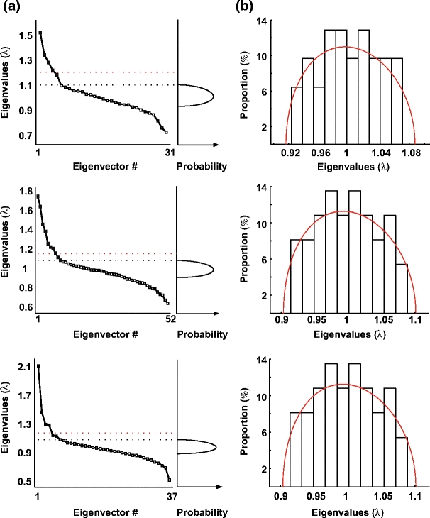
Evidence for signal components in the data sets. (a) Distribution of the eigenvalues for three example sessions (left) to be compared with the Marc̆enko-Pastur theoretical distribution (right). The upper bound of this theoretical distribution is indicated in the left panel with black dotted lines. The red dotted line indicates the upper bound derived from Tracy-Widom distribution for the highest eigenvalues in case of finite data sets (see text). (b) Histograms of the spectra of all the eigenvalues for each of the same 3 data sets as for panels in A after shuffling. The empirical distribution was in good agreement with the Marc̆enko-Pastur distribution, even without taking the Tracy-Widom correction into account. In particular, all computed eigenvalues remained within the theoretical bounds

Average reactivation

For sake of simplicity, let us first compute reactivation strengths using the TEMPLATE epoch as the MATCH epoch as well. In this case, at a time t, the standardized population vector is written . Let W _t be defined as . W _t can be decomposed in a diagonal matrix and the remaining matrix , therefore:

17

whence,

18

By definition, and thus which thus gives:

19

In the case where the MATCH epoch is different from the TEMPLATE, we have:

20

As mentioned above, memory trace reactivation studies aim at comparing awake activity (the TEMPLATE epoch here is the AWAKE epoch) with the subsequent sleep epoch (POST epoch, taking the role of the MATCH epoch). In Fig. 2 the epoch-wide time course of R for an example principal component from a recording of an ensemble of mPFC neurons is displayed for the PRE and POST epochs. Transient peaks can be observed that are much stronger in POST, and concentrated in the periods of identified slow wave sleep (SWS) (Peyrache et al. 2009). However, the baseline level is comparable between PRE and POST epochs. For this reason, from this point on, sleep epochs will always refer to SWS only. The SWS preceding the AWAKE epoch is taken as a control (PRE epoch). The variable (resp. ) quantifies the amount of variance that a given eigenvector from AWAKE could explain during the PRE epoch (resp. POST). The empirical distribution of (resp. ) as a function of λ_l is shown in Fig. 3(a). During POST, γ _l was more correlated to λ_l than in PRE, indicating that the correlation structure is more similar to that measured during AWAKE than it is in PRE. Note that, if it held that C ^POST = C ^AWAKE, then for all l. In general, this is not the case, for example, because the sleep correlation structure includes patterns that are characteristic of that behavioral phase, and these do not appear during the AWAKE epoch. In any event, during POST the regression line between λ_l and the corresponding values of γ _l has a steeper (and closer to 1) slope, indicating that the POST correlation matrix is more similar to its AWAKE analog than the one computed for PRE. Figure 3(b) shows an eigenvector-by-eigenvector (combined across sessions) comparison of the reactivation strengths during PRE and POST. While it is apparent that some reactivation strengths appear during PRE as well, most eigenvectors showed a larger value for POST, especially for eigenvectors associated to large eigenvalues. During PRE, reactivation strengths were nevertheless still important. This could be due, as mentioned above, to structural correlations, as well as to neural processes reflecting anticipation of the upcoming task (or perhaps lingering reactivations of yet earlier experiences).

Fig. 2.

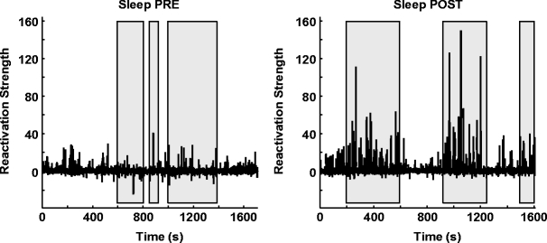
Example of reactivation strength time course (bins of 100 ms) for one principal component extracted from awake activity during two sleep sessions. Shaded areas denote periods of identified Slow Wave Sleep (SWS). POST SWS is dominated by brief, sharp increases in the reactivation strength, indicating strong similarity between instantaneous coactivations and the correlation pattern of the awake principal component

Fig. 3.

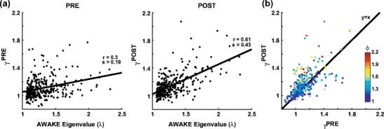
Eigenvectors from AWAKE better match activity in sleep POST than in PRE. (a) Eigenvalues from the AWAKE correlation matrix (x-axis) plotted against the average reactivation strength represented by the very same vectors during sleep PRE (left) and POST (right) for signal components only (). Each dot represents one of the 323 signal components identified from 63 datasets (four rats). Correlation values (r) and slopes (s) are indicated for the two distributions. The two measures were more strongly correlated during POST, and the slope of the linear regression line was steeper too (p < 10^− 6). (b) Average reactivation strength from POST versus PRE. Encoding strength is color coded. The points tend to lie above the line representing the identity function, showing that mean reactivation was stronger during POST. This effect was stronger for components with higher encoding strength

Distribution of R

In exploring the time course of the reactivation measure R, one interesting question that emerges is the nature of its variability. One possibility is that R fluctuates steadily around an average value (possibly different for each epoch), as would be the case, for example, if the underlying spike trains were a gaussian process. Alternatively, power-law behavior for the distribution of R values would indicate that the temporal evolution of R is dominated by strong transients, as it would result, for example, from “avalanche” dynamics (Beggs and Plenz 2003, 2004; Levina et al. 2007). In fact, if spike trains are multivariate normally distributed variables, the distribution of R can be computed and compared with experimental data. Let us consider the case in which the TEMPLATE activity is considered fixed, and we shall compute the distribution of R when the columns of the Q ^MATCH matrix are drawn from a multivariate normal distribution with covariance matrix C, .

In this case, for m different time bins, Q is a m ×N matrix and W = Q ^T Q is a N ×N matrix drawn from the so-called Wishart distribution with m degrees of freedom, . It can be shown that, for any given N-dimensional vector z:

21

where In particular, if z = p ^l, and C = C ^TEMPLATE it leads to:

22

Let assume that for the population vector the Q _it are drawn from a multivariate normal distribution: where C is the covariance matrix of the multivariate distribution (as the columns of Q are by definition z-transformed, C is also the correlation matrix). From Eq. (13), R _l could be written as:

23

where D is a diagonal matrix whose elements are The two terms on the right side of Eq. (23) should be considered separately: and . First, α(t) is easily deduced from Eq. (22)

24

25

26

where follows a Wishart distribution with a degree of freedom of 1 such that in the case C = C ^TEMPLATE.

The “auto correlation” term β(t) is a weighted sum of χ ² distributed variables whose number of degrees of freedom is not known a priori:

27

28

A common approximation (Imhof 1961) of a weighted sum of chi-squares is a gamma distribution whose first two moments are the same as those of the sum. For a gamma distribution of shape parameter k and scale parameter θ, this gives (with the superscript of p ^l omitted):

29

which leads to (recalling that ):

30

hence, β is equivalent to1

31

Finally, if α and β are assumed independent, the theoretical distributions of and are:

32

33

This result leads to an important conclusion: even if α and β were correlated, the tail of the distribution could not be “heavier” or more skewed than an exponential distribution. Nevertheless, as we shall see in the following section, experimental evidence shows that those distributions are actually power-laws. The distribution of R ^{TE − TE} for the first eigenvectors of the 3 data sets presented in Fig. 1 are plotted in Fig. 4(a), against the theoretical curve (red) and the result from multivariate normal data simulations (blue). The very same distributions are shown in log-log scales in Fig. 4(b) to highlight the power-law tails of the distributions. The higher the encoding strength (λ/λ_max), the better the tail is fitted with a power-law (in other words the tail is linear in log-log plots). Figure 4(c) shows the theoretical (under the multivariate normal hypothesis) and empirical distribution for the individual terms α and β.

Fig. 4.

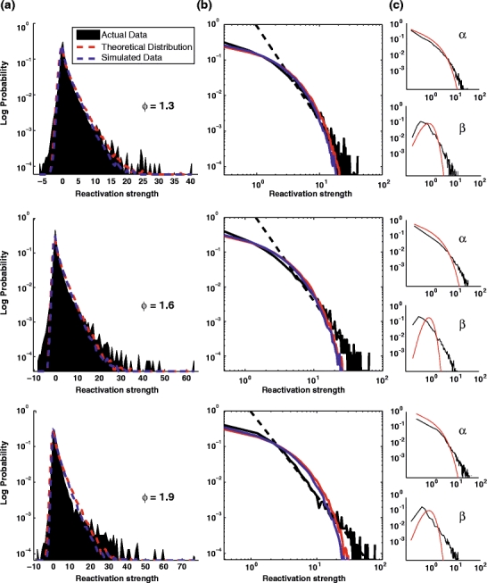
Distribution of the R measure during the TEMPLATE epochs (R ^{TE − TE}). Data are from the same three sessions as in Fig. 1 (AWAKE). (a) Distribution of R across all time bins for the first principal component of each of the three sessions (representative of the dataset, the respective encoding strength are displayed on top of the distributions). Real data (black), theoretical expectation (red) derived from a Monte-Carlo sampling of Eq. (32) (n = 10⁵), and a numerical simulation using normal multivariate data with the same correlation matrix as the actual data (blue). (b) Same plots as A but in log-log scale. (c) Distribution of the α and β terms from Eq. (32). High encoding strength eigenvectors (e.g. one at bottom) tend to exhibit a clear power-law distribution of their R measure distribution

Reactivation is a rare event

The significant increase of the average of reactivation measures from PRE sleep to POST sleep (Fig. 3(c), see also Peyrache et al. 2009) might not be the most relevant parameter which changes with learning. Indeed, as shown in Fig. 2, the reactivation measure shows prominent transient ‘spikes’ during POST sleep associated with a simultaneous increase in firing of the cells associated with the highest weights in the principal component. During POST, reactivation strength distributions deviate strongly from the multivariate normal case, and their tail can be well fit with a power law (Fig. 5). Such deviation from the theoretical distribution is less marked during PRE, despite some hints of power law behavior.

Fig. 5.

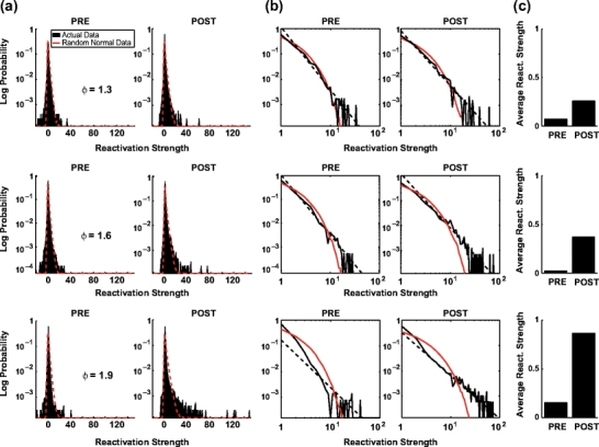
Distribution of the R measure during the MATCH epochs (PRE and POST). Data are from the same three principal components as in Fig. 4 (AWAKE). (a) Distribution of R for PRE (left) and POST (right) sleep of the real data (black) and the theoretical expectation (red) derived from a Monte-Carlo sampling of Eq. (33) (n = 10⁵). (b) Same plots as (a) but in log-log scale showing a clear power law decay in sleep POST for high encoding strength components (second and third rows). (c) Bar plot of average of the distributions of actual data shown in (a) and (b) for PRE (left) and POST (right). Note that the average reactivation strength is equal to γ − 1. The difference in the means seemed to be related to the difference in the tails of the distributions

In principle, the heavier tail of the reactivation strength distribution during POST observed in Fig. 5 could result from an increase in variability over the global population instantaneous firing rate. The standardization of the binned spike trains for each cell (corresponding to the rows of the Q matrix), does not prevent the instantaneous firing rate from varying considerably, for example because of UP/DOWN states bistability dominating cortical activity during sleep (Steriade 2006). In order to control for this possibility, we computed the reactivation strength from shuffled data where, for each time bin, the identity of the cells was randomly permuted. This shuffling procedure preserves the instantaneous global firing rate (and its fluctuations), but it destroys the patterns of co-activation. In Fig. 6(a), from the same session presented in Fig. 2, the reactivation measure was computed for one principal component while the eigenvector weights (or equivalently, the identities of the cells in the multi-unit spike train ) were shuffled 1000 times. The 99th percentile of the resulting distribution, for each time bin, is shown as the grey curve superimposed upon actual reactivation measure data (black dots). Those points are plotted as a function of the average firing rate (in z-score) which represent the global activation of the cell population. There is a relation between instantaneous global activation and the upper bound of the distribution of shuffled measures (the 99th percentile) which is similar in PRE and POST sleep. Nevertheless, while the actual reactivation measure remained within the expected bounds in PRE sleep (only 1% of the bins exceeded the shuffled measure), the actual reactivation measure largely exceeded this confidence interval in POST sleep (3.4% of the bins were above the 99th percentile). To check whether this could be due to a difference in global population activation, the PRE and POST sleep distribution of average z-score were compared (right inset) and, indeed, showed no difference (Kolmogorov-Smirnov test, p = 0.11).

Fig. 6.

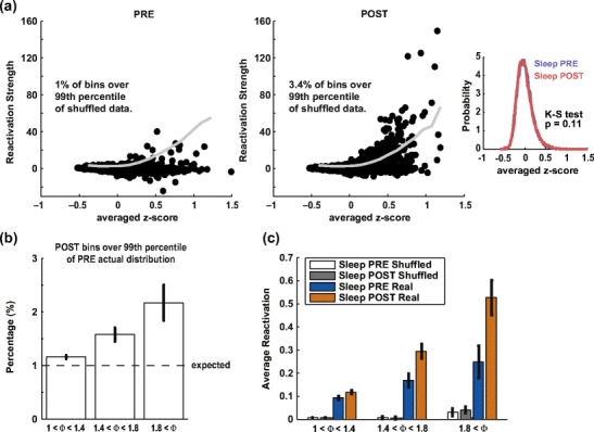
Effect of instantaneous global fluctuations of firing rate on the reactivation strength measure. (a) For one principal component recorded during one session (third example of Figs. 1, 4 and 5), the scatterplots show the dependence between the instantaneous activation (expressed as the instantaneous z-score averaged over all recorded cells) and the corresponding reactivation strength. In black, the actual data are shown, vs. the 99th percentile of the shuffled control. The data pertain to the PRE epoch (left) and the POST epoch (right). In POST, but not in PRE, a larger number (3.4%) of points than expected by chance is above the 99th percentile, showing that reactivation effects are not likely to be the product of activity fluctuations alone. Meanwhile, 4.5% of POST bins were above the 99th percentile of the PRE distribution. Right inset: Distribution of the averaged z-score, measuring the degree of instantaneous population activity, for all time bins in PRE (blue) and POST (red) sleep. The two distributions are not different. (b) Pooled data of the number of POST bins exceeding the 99th percentile of PRE distributions. Signal components were grouped according to their encoding strength. The percentages were significantly over 1% for the three groups (p < 0.05, t-test) and, individually, percentages were correlated with encoding strengths (r = 0.39, p < 10^− 12). (c) Pooled data from all principal components computed from all available recording sessions comparing the reactivation measure average for sleep PRE and POST with shuffled measures for the two same epochs. The difference between PRE and POST sleep epochs was significant for the three signal groups (p < 0.05, paired t-test), but not for shuffled measures. Furthermore, the averages for shuffled data were one order of magnitude less than actual measures

This difference in the tail of the distribution is very important for the excess reactivation strength in POST with respect to PRE which we take as evidence for memory replay. In the example of Fig. 6(a), 4.5% of the bins from POST exceeded the 99th percentile of the PRE distribution. Hence, the difference in tails of PRE and POST distributions (as in the examples in Fig. 5) resulted in a higher probability for reactivation strength values from POST sleep to exceed the 99th percentile of the PRE reactivation strength distribution than the expected 1% (Fig. 6(b)) in an encoding strength dependent manner: the percentage of “outliers” is significantly above chance for all groups of components and it increases with encoding strength. Whereas average actual reactivation strength differences between PRE and POST (Fig. 6(c), significant for all groups, p < 0.05, t-test) show the same profile as the increased number of outliers in POST sleep (Fig. 6(b)), there was no difference in mean of the shuffled reactivation strengths. Furthermore, reactivation strengths for shuffled data were on average one order of magnitude smaller than reactivation strengths computed from actual data.

These brief, sharp increases in the reactivation strength time course (Fig. 2, or similarly the outliers in the distribution from POST) accounted for a large part of the difference between the average reactivation strengths. This can be seen in the cumulative contributions:

34

whose difference between POST sleep and PRE sleep is shown in Fig. 7. The patterns were grouped according to encoding strength (). For distributions P(u) with an exponential tail, this function will reach an asymptotic value, indicating that large values contribute little to the overall average. Diverging values of (e.g. ∝ log(r)), are indicative of a P(u) with a tail decaying with a power law. This function converges asymptotically to a value equal to the difference of the average reactivation strength between POST and PRE (also equal to γ ^POST − γ ^PRE). The black diamonds indicate the 99th percentile of the distribution of POST sleep reactivation distribution. Hence, up to half of the difference (for the highest encoding strength) between POST and PRE sleep average of reactivation strength is due to one percent of the time bins from POST sleep, that is, the bins in which the transient reactivation events took place.

Fig. 7.

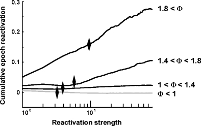
Cumulative average computed with Eq. (34) for components of the whole data sets separated in the same four groups as in Fig. 6. Black diamonds display the 99th percentile of the POST distribution. This shows that for the highest encoding strength, half of the difference between PRE and POST (represented by the asymptotic value of each curve) is explained by only 1% of the bins of POST sleep

Interactions between different cell assemblies

Different principal components, referring to the same data, tend to activate at different times, and their activation is concomitant with the firing of independent cell groups (Fig. 8(a)). Interestingly, as shown in Fig. 8(b), the time courses of R for the two principal components show a trough for zero-lag in the cross-correlation, showing that the simultaneous activation of the two components was less likely than in the case of uncorrelated time course. This effect was observed for all pairs of principal components compute from the same sessions (Peyrache et al. 2009).

Fig. 8.

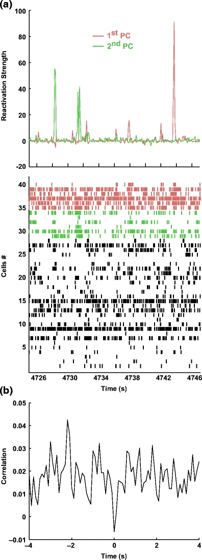
Interaction between two simultaneous reactivation strengths. (a) Example of reactivation strength timecourse for two signal components from the same session during SWS (top) with the simultaneous cell activity (raster plot, bottom; each row represents the spike train from one cell). The red and green rasters (respective to the colored reactivation strength traces) show the spike activity of the six cells associated with the highest weights in each component (i.e. with the highest contribution, see below). Other spike trains (in black) are displayed in random order. Each peak of the reactivation strengths is associated with a transient increase of firing rates of the cells with the highest weights in the respective component. (b) Cross-correlogram of the reactivation strengths for the two components during SWS showing marked negativity at 0 lag

Peaks of R correspond to transient synchronization, or co-firing, of cells with same-signed weights in the principal vector. Nevertheless, each spike train participates differently to any particular reactivation strength, likely depending on its associated weight in the principal component. To quantify the contribution of the kth cell, the reactivation strength was computed with ∀ t, Q _kt = 0 , or by removing the terms depending on Q _kt in Eq. (13):

35

then the contribution was defined as:

36

the normalization factor 1/2 has been derived from simple calculation so that

37

Figure 9(a) shows an example of the distribution of the contribution for two signal components in a single day. The joint distribution of individual cells’ contributions to those two patterns (Fig. 9(b)) indicates no overlap between identities of highly influential cells.

Fig. 9.

Contribution of individual spike trains to the overall reactivation strength. (a) Contribution of all the cells recorded during one session to the average of R ₁ (or R ₂), the reactivation strength of the first (or second) component, as a function of PC weights for the first (resp. the second) principal components p ¹ (or p ²). (b) Scatter plot of the contributions to R ₁ (x-axis) and R ₂ shows that the sets of high-contribution cells for the two components are virtually disjoint

Discussion

This study shows that a simple and linear pattern separation method such as PCA can be powerful in the identification and characterization of cell assemblies in brain recordings. This is an important part of the study of the replay phenomenon, where two epochs must be compared, one in which assemblies would be encoded, and another one, in which the same assemblies might be replayed again. By construction, our method is a simple extension of the seminal work of Bruce McNaughton and co-workers (Wilson and McNaughton 1994; Kudrimoti et al. 1999), offering two important new features: first, a detailed time course for replay is obtained, at the scale of the chosen temporal bin (100 ms in the present study). The resulting resolution is much finer than what can be achieved if replay is only measured from the similarity between the epoch-wide correlation matrices. This has important consequences for the study of the physiology of replay. In particular, we have found that replay takes place for the most part in discrete, transient events (see e.g. Figs. 2 and 5), which correspond to the coordinated activation of subgroups of cells. In fact, such transients mostly take place during UP states characteristic of slow-wave sleep. These are periods of elevated, relatively steady activation, when measured at the level of the global neuronal population. However, a very different time course is uncovered when we consider the dynamics of subgroups of cells, defined by co-activations measured during wakefulness: a avalanche-like dynamics (Beggs and Plenz 2003, 2004; Levina et al. 2007), which is embedded in a generally more regular population dynamics. Moreover, a detailed view of temporal evolution of replay has allowed to explore the links between this phenomenon on one hand and hippocampal sharp waves (crucial for hippocampal replay (Kudrimoti et al. 1999)) and UP-DOWN state transitions on the other, showing how replay is an integral part of hippocampal-cortical interactions and sleep physiology (Peyrache et al. 2009).

Second, PCA allows to tease apart the dynamics of different cell assemblies, corresponding to different principal components. Interestingly, distinct subgroups tend to seldom reactivate at the same instant, suggesting that some sort of pattern separation mechanism may take place during sleep. Because the time courses of the different principal components are un- (or anti-)correlated (Fig. 8), separating them allows to reveal details of the temporal evolution which would be otherwise averaged out, for example, the transients discussed above.

This measure also lends itself to rigorous mathematical analysis, making some inroads towards precisely defined null hypotheses to be tested against the experimental results. The known eigenvalue spectrum of correlation matrices from purely random data (Marčenko and Pastur 1967; Sengupta and Mitra 1999) allows determination of which of the principal components in a given data set are likely to carry meaningful information; in the data considered here, up to 5 or 6 PCs can be found in a simultaneous recording of 30–50 neurons (Fig. 1). This could be seen as a generalization in N dimensions of the classical Pearson test for pairwise correlations. The boundaries of the support of the theoretical distribution for the eigenvalues, λ_min and λ_max, can be taken as the critical value for the rejection of the null hypothesis. In the range of parameters corresponding to our practical experimental situation (number of variables, N ~ 50, number of time bins, b ~10⁴ for a bin size of 100 ms) these boundaries are sharp, as demonstrated by the Tracy-Widom estimate of the variance of the distribution of the largest eigenvalue (Tracy and Widom 1994). Thus, an analysis procedure that considers as ‘signal’ the principal components associated to an eigenvalue larger than λ_max is justified from the theoretical point of view. This allows us to identify certain principal components as signal-carrying cell assemblies.

In the next stage of the analysis, the R measure is computed, measuring the time course of replay during the PRE and the POST epoch. In principle, replay could be the result of a continuous process, for example one that modified the probability of co-activation of cell pairs, as a consequence of synaptic modification. In this case, one would expect an exponentially tailed distribution for the R values. This was indeed verified analytically, under the hypothesis of multivariate, normally distributed data.

Reactivation strengths are greater than chance levels both in PRE and POST sleep. This could be due to structural correlations, pre-encoded in the synaptic matrix. Such correlations would be present in ensemble activity at all times, both in spontaneous and in behaviorally evoked activity, and would not have to encode any task-relevant information. It is also possible that, during PRE sleep, the prefrontal cortex is already engaged in processes anticipatory of the task. This could explain the similarities between the activity in the PRE and AWAKE epochs.

Nevertheless, POST sleep shows a significantly greater degree of replay. This can be observed by empirically comparing the R distributions for PRE and POST. Interestingly, most of the difference between PRE and POST is accounted for by the very large data points in the tail of the distribution, so that, for the principal components associated to the largest eigenvalues, up to 50% of the difference is accounted for by only the largest 1% of the points. It seems therefore likely that the large transients in the replay measure are at least in part a consequence of replay. Moreover, it is possible that during experience, synaptic plasticity operates by modifying and strengthening existing cell assemblies (during gradual learning for example), as opposed to creating new ones from scratch. This would also contribute to explain why reactivation strength for the same eigenvectors may be high both in PRE and POST (albeit stronger in POST).

Our method, in its current version, has some limitations. For one, it does not provide a way to directly discount structural correlation patterns present in the PRE epoch from the templates extracted by the AWAKE epoch, which would obviate the need for a comparison of the empirical PRE and POST distributions. Also, it would be important to compute analytical bounds for quantities under null hypotheses less stringent than that of multivariate normal spike trains. Still this technique has already led to scientific results of relevance (Peyrache et al. 2009): as another example of use of this technique, as mentioned above, the sleep epoch can serve as a template for detecting matches in the awake epoch: we extracted patterns from PCA applied to the POST epoch, and matched them on the activity during the AWAKE epoch. This allowed us to assess which behavioral phases of the task were represented the most in the sleep activity (and possibly, be preferentially consolidated). We concluded that this coincided with activity at the “choice point” of the maze, i.e. the fork of the Y-maze where the animal had to commit to a potentially costly choice. Also, the effect depended upon learning: sleep-derived activity patterns were more concentrated at the decision point after the rat acquired the rule governing reward (Peyrache et al. 2009). These initial results provide hope that this method, for its relative simplicity and ease of approach with mathematical tools, may spur further experimental and analytical work.

References

- Beggs JM, Plenz D. Neuronal avalanches in neocortical circuits. Journal of Neuroscience. 2003;23(35):11167–11177. doi: 10.1523/JNEUROSCI.23-35-11167.2003. [DOI] [PMC free article] [PubMed] [Google Scholar]
- Beggs JM, Plenz D. Neuronal avalanches are diverse and precise activity patterns that are stable for many hours in cortical slice cultures. Journal of Neuroscience. 2004;24(22):5216–5229. doi: 10.1523/JNEUROSCI.0540-04.2004. [DOI] [PMC free article] [PubMed] [Google Scholar]
- Benchenane, K., Peyrache, A., Khamassi, M., Battaglia, F. P., & Wiener, S. I. (2008). Coherence of theta rhythm between hippocampus and medial prefrontal cortex modulates prefrontal network activity during learning in rats. Soc Neuroscie Abstr, 690.15.
- Biroli G, Bouchaud JP, Potters M. On the top eigenvalue of heavy-tailed random matrices. EPL (Europhysics Letters. 2007;78(1):10001. doi: 10.1209/0295-5075/78/10001. [DOI] [Google Scholar]
- Bishop CM. Neural networks for pattern recognition. New York: Oxford University Press; 1995. [Google Scholar]
- Bourlard H, Kamp Y. Auto-association by multilayer perceptrons and singular value decomposition. Biological Cybernetics. 1988;59(4):291–294. doi: 10.1007/BF00332918. [DOI] [PubMed] [Google Scholar]
- Buzsáki G. Large-scale recording of neuronal ensembles. Nature Neuroscience. 2004;7(5):446–451. doi: 10.1038/nn1233. [DOI] [PubMed] [Google Scholar]
- Chapin JK, Nicolelis MA. Principal component analysis of neuronal ensemble activity reveals multidimensional somatosensory representations. Journal of Neuroscience Methods. 1999;94(1):121–140. doi: 10.1016/S0165-0270(99)00130-2. [DOI] [PubMed] [Google Scholar]
- Euston DR, Tatsuno M, Mcnaughton BL. Fast-forward playback of recent memory sequences in prefrontal cortex during sleep. Science. 2007;318(5853):1147–1150. doi: 10.1126/science.1148979. [DOI] [PubMed] [Google Scholar]
- Fujisawa S, Amarasingham A, Harrison MTT, Buzsáki G. Behavior-dependent short-term assembly dynamics in the medial prefrontal cortex. Nature Neuroscience. 2008;11:823–833. doi: 10.1038/nn.2134. [DOI] [PMC free article] [PubMed] [Google Scholar]
- Geisler C, Robbe D, Zugaro M, Sirota A, Buzsáki G. Hippocampal place cell assemblies are speed-controlled oscillators. Proceedings of the National Acadademy of Science of the United States of America. 2007;104(19):8149–8154. doi: 10.1073/pnas.0610121104. [DOI] [PMC free article] [PubMed] [Google Scholar]
- Harris KD, Csicsvari J, Hirase H, Dragoi G, Buzsáki G. Organization of cell assemblies in the hippocampus. Nature. 2003;424(6948):552–556. doi: 10.1038/nature01834. [DOI] [PubMed] [Google Scholar]
- Hebb DO. The organization of behavior: A neuropsychological theory. New York: Wiley; 1949. [Google Scholar]
- Ikegaya Y, Aaron G, Cossart R, Aronov D, Lampl I, Ferster D, et al. Synfire chains and cortical songs: Temporal modules of cortical activity. Science. 2004;304(5670):559–564. doi: 10.1126/science.1093173. [DOI] [PubMed] [Google Scholar]
- Imhof JP. Computing the distribution of quadratic forms in normal variables. Biometrika. 1961;48(3–4):419–426. [Google Scholar]
- Ji D, Wilson MA. Coordinated memory replay in the visual cortex and hippocampus during sleep. Nature Neuroscience. 2006;10(1):100–107. doi: 10.1038/nn1825. [DOI] [PubMed] [Google Scholar]
- Kudrimoti HS, Barnes CA, McNaughton BL. Reactivation of hippocampal cell assemblies: Effects of behavioral state, experience, and eeg dynamics. Journal of Neuroscience. 1999;19(10):4090–4101. doi: 10.1523/JNEUROSCI.19-10-04090.1999. [DOI] [PMC free article] [PubMed] [Google Scholar]
- Lee AK, Wilson MA. Memory of sequential experience in the hippocampus during slow wave sleep. Neuron. 2002;36(6):1183–1194. doi: 10.1016/S0896-6273(02)01096-6. [DOI] [PubMed] [Google Scholar]
- Levina A, Herrmann JM, Geisel T. Dynamical synapses causing self-organized criticality in neural networks. Nature Physics. 2007;3(12):857–860. doi: 10.1038/nphys758. [DOI] [Google Scholar]
- Louie K, Wilson MA. Temporally structured replay of awake hippocampal ensemble activity during rapid eye movement sleep. Neuron. 2001;29(1):145–156. doi: 10.1016/S0896-6273(01)00186-6. [DOI] [PubMed] [Google Scholar]
- Marr D. Simple memory: A theory for archicortex. Philosophical transactions of the Royal Society of London. Series B, Biological Sciences. 1971;262(841):23–81. doi: 10.1098/rstb.1971.0078. [DOI] [PubMed] [Google Scholar]
- Marčenko VA, Pastur LA. Distribution of eigenvalues for some sets of random matrices. Mathematics of the USSR-Sbornik. 1967;1(4):457–483. doi: 10.1070/SM1967v001n04ABEH001994. [DOI] [Google Scholar]
- McNaughton BL, O’Keefe J, Barnes CA. The stereotrode: A new technique for simultaneous isolation of several single units in the central nervous system from multiple unit records. Journal of Neuroscience Methods. 1983;8(4):391–397. doi: 10.1016/0165-0270(83)90097-3. [DOI] [PubMed] [Google Scholar]
- Mokeichev A, Okun M, Barak O, Katz Y, Ben-Shahar O, Lampl I. Stochastic emergence of repeating cortical motifs in spontaneous membrane potential fluctuations in vivo. Neuron. 2007;53(3):413–425. doi: 10.1016/j.neuron.2007.01.017. [DOI] [PubMed] [Google Scholar]
- Nádasdy Z, Hirase H, Czurkó A, Csicsvari J, Buzsáki G. Replay and time compression of recurring spike sequences in the hippocampus. Journal of Neuroscience. 1999;19(21):9497–9507. doi: 10.1523/JNEUROSCI.19-21-09497.1999. [DOI] [PMC free article] [PubMed] [Google Scholar]
- Nadel L, Moscovitch M. Memory consolidation, retrograde amnesia and the hippocampal complex. Current Opinion in Neurobiology. 1997;7(2):217–227. doi: 10.1016/S0959-4388(97)80010-4. [DOI] [PubMed] [Google Scholar]
- Nicolelis MA, Baccala LA, Lin RC, Chapin JK. Sensorimotor encoding by synchronous neural ensemble activity at multiple levels of the somatosensory system. Science. 1995;268(5215):1353–1358. doi: 10.1126/science.7761855. [DOI] [PubMed] [Google Scholar]
- Oja E. A simplified neuron model as a principal component analyzer. Journal of Mathematical Biology. 1982;15(3):267–273. doi: 10.1007/BF00275687. [DOI] [PubMed] [Google Scholar]
- Pipa G, Wheeler DW, Singer W, Nikolić D. Neuroxidence: Reliable and efficient analysis of an excess or deficiency of joint-spike events. Journal of Computational Neuroscience. 2008;25(1):64–88. doi: 10.1007/s10827-007-0065-3. [DOI] [PMC free article] [PubMed] [Google Scholar]
- Peyrache A, Khamassi M, Benchenane K, Wiener SI, Battaglia FP. Replay of rule learning-related patterns in the prefrontal cortex during sleep. Nature Neuroscience. 2009 doi: 10.1038/nn.2337. [DOI] [PubMed] [Google Scholar]
- Ribeiro S, Gervasoni D, Soares ES, Zhou Y, Lin SC, Pantoja J, et al. Long-lasting novelty-induced neuronal reverberation during slow-wave sleep in multiple forebrain areas. PLoS Biology. 2004;2(1):24. doi: 10.1371/journal.pbio.0020024. [DOI] [PMC free article] [PubMed] [Google Scholar]
- Riehle A, Grun S, Diesmann M, Aertsen A. Spike synchronization and rate modulation differentially involved in motor cortical function. Science. 1997;278(5345):1950–1953. doi: 10.1126/science.278.5345.1950. [DOI] [PubMed] [Google Scholar]
- Scoville WB, Milner B. Loss of recent memory after bilateral hippocampal lesions. Journal of Neurology, Neurosurgery and Psychiatry. 1957;20(11):11–21. doi: 10.1136/jnnp.20.1.11. [DOI] [PMC free article] [PubMed] [Google Scholar]
- Sengupta AM, Mitra PP. Distributions of singular values for some random matrices. Physical Review E. 1999;60(3):3389. doi: 10.1103/PhysRevE.60.3389. [DOI] [PubMed] [Google Scholar]
- Squire LR, Zola-Morgan S. The medial temporal lobe memory system. Science. 1991;253(5026):1380–1386. doi: 10.1126/science.1896849. [DOI] [PubMed] [Google Scholar]
- Steriade M. Grouping of brain rhythms in corticothalamic systems. Neuroscience. 2006;137:1087–1106. doi: 10.1016/j.neuroscience.2005.10.029. [DOI] [PubMed] [Google Scholar]
- Tracy C, Widom H. Level-spacing distributions and the airy kernel. Communications in Mathematical Physics. 1994;159(1):151–174. doi: 10.1007/BF02100489. [DOI] [Google Scholar]
- Wigner EP. Characteristic vectors of bordered matrices with infinite dimensions. The Annals of Mathematics. 1955;62(3):548–564. doi: 10.2307/1970079. [DOI] [Google Scholar]
- Wilson MA, McNaughton BL. Reactivation of hippocampal ensemble memories during sleep. Science. 1994;265(5172):676–679. doi: 10.1126/science.8036517. [DOI] [PubMed] [Google Scholar]
- Wilson RI, Laurent G. Role of gabaergic inhibition in shaping odor-evoked spatiotemporal patterns in the drosophila antennal lobe. The Journal of Neuroscience. 2005;25(40):9069–9079. doi: 10.1523/JNEUROSCI.2070-05.2005. [DOI] [PMC free article] [PubMed] [Google Scholar]