A Principled Approach to Deriving Approximate Conditional Sampling Distributions in Population Genetics Models with Recombination

Abstract

The multilocus conditional sampling distribution (CSD) describes the probability that an additionally sampled DNA sequence is of a certain type, given that a collection of sequences has already been observed. The CSD has a wide range of applications in both computational biology and population genomics analysis, including phasing genotype data into haplotype data, imputing missing data, estimating recombination rates, inferring local ancestry in admixed populations, and importance sampling of coalescent genealogies. Unfortunately, the true CSD under the coalescent with recombination is not known, so approximations, formulated as hidden Markov models, have been proposed in the past. These approximations have led to a number of useful statistical tools, but it is important to recognize that they were not derived from, though were certainly motivated by, principles underlying the coalescent process. The goal of this article is to develop a principled approach to derive improved CSDs directly from the underlying population genetics model. Our approach is based on the diffusion process approximation and the resulting mathematical expressions admit intuitive genealogical interpretations, which we utilize to introduce further approximations and make our method scalable in the number of loci. The general algorithm presented here applies to an arbitrary number of loci and an arbitrary finite-alleles recurrent mutation model. Empirical results are provided to demonstrate that our new CSDs are in general substantially more accurate than previously proposed approximations.

THE probability of observing a sample of DNA sequences under a given population genetics model—which is referred to as the sampling probability or likelihood—plays an important role in a wide range of problems in a genetic variation study. When recombination is involved, however, obtaining an analytic formula for the sampling probability has hitherto remained a challenging open problem (see Jenkins and Song 2009, 2010 for recent progress on this problem). As such, much research (Griffiths and Marjoram 1996; Kuhner et al. 2000; Nielsen 2000; Stephens and Donnelly 2000; Fearnhead and Donnelly 2001; De Iorio and Griffiths 2004a,b; Fearnhead and Smith 2005; Griffiths et al. 2008; Wang and Rannala 2008) has focused on developing Monte Carlo methods on the basis of the coalescent with recombination (Griffiths 1981; Kingman 1982a,b; Hudson 1983), a well-established mathematical framework that models the genealogical history of sample chromosomes. These Monte Carlo-based full-likelihood methods mark an important development in population genetics analysis, but a well-known obstacle to their utility is that they tend to be computationally intensive. For a whole-genome variation study, approximations are often unavoidable, and it is therefore important to think of ways to minimize the trade-off between scalability and accuracy.

A popular likelihood-based approximation method that has had a significant impact on population genetics analysis is the following approach introduced by Li and Stephens (2003): Given a set Φ of model parameters (e.g., mutation rate, recombination rate, etc.), the joint probability p(h₁, … , h_n | Φ) of observing a set {h₁, … , h_n} of haplotypes sampled from a population can be decomposed as a product of conditional sampling distributions (CSDs), denoted by π,

(1)

where π(h_k+1|h₁, …, h_k, Φ) is the probability of an additionally sampled haplotype being of type h_k+1, given a set of already observed haplotypes h₁, …, h_k. In the presence of recombination, the true CSD π is unknown, so Li and Stephens proposed using an approximate CSD in place of π, thus obtaining the following approximation of the joint probability:

(2)

Li and Stephens referred to this approximation as the product of approximate conditionals (PAC) model. In general, the closer is to the true CSD π, the more accurate the PAC model becomes. Notable applications and extensions of this framework include estimating crossover rates (Li and Stephens 2003; Crawford et al. 2004) and gene conversion parameters (Gay et al. 2007; Yin et al. 2009), phasing genotype data into haplotype data (Stephens and Scheet 2005; Scheet and Stephens 2006), imputing missing data to improve power in association mapping (Stephens and Scheet 2005; Li and Abecasis 2006; Marchini et al. 2007; Howie et al. 2009), inferring local ancestry in admixed populations (Price et al. 2009), inferring human colonization history (Hellenthal et al. 2008), inferring demography (Davison et al. 2009), and so on.

Another problem in which the CSD plays a fundamental role is importance sampling of genealogies under the coalescent process (Stephens and Donnelly 2000; Fearnhead and Donnelly 2001; De Iorio and Griffiths 2004a,b; Fearnhead and Smith 2005; Griffiths et al. 2008). In this context, the optimal proposal distribution can be written in terms of the CSD π (Stephens and Donnelly 2000), and as in the PAC model, an approximate CSD may be used in place of π. The performance of an importance sampling scheme depends critically on the proposal distribution and therefore on the accuracy of the approximation . Often in conjunction with composite-likelihood frameworks (Hudson 2001; Fearnhead and Donnelly 2002), importance sampling has been used in estimating fine-scale recombination rates (McVean et al. 2004; Fearnhead and Smith 2005; Johnson and Slatkin 2009).

So far, a significant scope of intuition has gone into choosing the approximate CSDs used in these problems (Marjoram and Tavaré 2006). In the case of completely linked loci, Stephens and Donnelly (2000) suggested constructing an approximation by assuming that the additional haplotype h_k+1 is an imperfect copy of one of the first k haplotypes, with copying errors corresponding to mutation. Fearnhead and Donnelly (2001) generalized this construction to include crossover recombination, assuming that the haplotype h_k+1 is an imperfect mosaic of the first k haplotypes (i.e., h_k+1 is obtained by copying segments from h₁, …, h_k, where crossover recombination can change the haplotype from which copying is performed). The associated CSD, which we denote by , can be interpreted as a hidden Markov model and so admits an efficient dynamic programming solution. Finally, Li and Stephens (2003) proposed a modification to Fearnhead and Donnelly's model that limits the hidden state space, thereby providing a computational simplification; we denote the corresponding approximate CSD by .

Although these approaches are computationally appealing, it is important to note that they are not derived from, though are certainly motivated by, principles underlying typical population genetics models, in particular the coalescent process (Griffiths 1981; Kingman 1982a,b; Hudson 1983). The main objective of this article is to develop a principled technique to derive an improved CSD directly from the underlying population genetics model. Rather than relying on intuition, we base our work on mathematical foundation. The theoretical framework we employ is the diffusion process. De Iorio and Griffiths (2004a,b) first introduced the diffusion-generator approximation technique to obtain an approximate CSD in the case of a single locus (i.e., no recombination). Griffiths et al. (2008) later extended the approach to two loci to include crossover recombination, assuming a parent-independent mutation model at each locus. In this article, we extend the framework to develop a general algorithm that applies to an arbitrary number of loci and an arbitrary finite-alleles recurrent mutation model.

Our work can be summarized as follows. Using the diffusion-generator approximation technique, we derive a recursion relation satisfied by an approximate CSD. This recursion can be used to construct a closed system of coupled linear equations, in which the conditional sampling probability of interest appears as one of the unknown variables. The system of equations can be solved using standard numerical analysis techniques. However, the size of the system grows superexponentially with the number of loci and, consequently, so does the running time. To remedy this drawback, we introduce additional approximations to make our approach scalable in the number of loci. Specifically, the recursion admits an intuitive genealogical interpretation, and, on the basis of this interpretation, we propose modifications to the recursion, which then can be easily solved using dynamic programming. The computational complexity of the modified algorithm is polynomial in the number of loci, and, importantly, the resulting CSD has little loss of accuracy compared to that following from the full recursion.

The accuracy of approximate CSDs has not been discussed much in the literature, except in the application-specific context for which they are being employed. In this article, we carry out an empirical study to explicitly test the accuracy of various CSDs and demonstrate that our new CSDs are in general substantially more accurate than previously proposed approximations. We also consider the PAC framework and show that our approximations also produce more accurate PAC-likelihood estimates. We note that for the maximum-likelihood estimation of recombination rates, the actual value of the likelihood may not be so important, as long as it is maximized near the true recombination rate. However, in many other applications—e.g., phasing genotype data into haplotype data, imputing missing data, importance sampling, and so on—the accuracy of the CSD and PAC-likelihood function over a wide range of parameter values may be important. Thus, we believe that the theoretical work presented here will have several practical implications; our method can be applied in a wide range of statistical tools that use CSDs, improving their accuracy.

The remainder of this article is organized as follows. To provide intuition for the ensuing mathematics, we first describe a genealogical process that gives rise to our CSD. Using our genealogical interpretation, we consider two additional approximations and relate these to previously proposed CSDs. Then, in the following section, we derive our CSD using the diffusion-generator approach and provide mathematical statements for the additional approximations; some interesting limiting behavior is also described there. This section is self-contained and may be skipped by the reader uninterested in mathematical details. Finally, in the subsequent section, we carry out a simulation study to compare the accuracy of various approximate CSDs and demonstrate that ours are generally the most accurate.

A GENEALOGICAL FORMULATION

Before delving into mathematical details, we first describe a genealogical interpretation for our proposed CSD. In addition to providing intuition about the underlying mathematics (which is discussed in detail in the following section), the genealogical interpretation suggests a tractable approximation of our CSD. We discuss how some previously proposed CSDs may also be viewed as approximations of our basic scheme.

Preliminary notation:

As our basic stochastic process, we consider a finite-sites, finite-alleles version of the coalescent with recombination. In particular, denote the set of loci by L = {1, …, k}. The following general notation is used hereafter to describe mutation and recombination events in the coalescent:

• Mutation: We use E_ℓ to denote the set of allele types at locus ℓ ∈ L. Mutation events at locus ℓ occur with rate θ_ℓ/2. Going forward in time, given that there is a mutation, a transition from allele a ∈ E_ℓ to allele a′ ∈ E_ℓ occurs with probability . By a parent-independent mutation (PIM) model, we mean a model in which for all a, a′, and ℓ.

• Recombination: The set of recombination breakpoints is denoted by B = {(1, 2), …, (k − 1, k)}. Given a breakpoint b = (ℓ, ℓ + 1) ∈ B, recombination events between loci ℓ and ℓ + 1 occur with rate ρ_b/2.

We use to denote the set of k-locus haplotypes. A sample configuration of haplotypes is specified by a vector , with n_h being the number of haplotypes of type h in the sample. The total number of haplotypes in n is denoted by . Finally, we use e_h to denote the singleton configuration with a 1 for haplotype h and 0's elsewhere.

Conditional sampling:

Recall that a realization of the coalescent with recombination is a random genealogy comprising a series of events (i.e., mutation, recombination, and coalescence), relating a collection of haplotypes. This genealogy results from a continuous-time Markov process, which moves backward through time and takes collections of haplotypes as states; we refer to a haplotype in the current state as a lineage. An event then corresponds to a jump in the continuous-time Markov process and makes a particular modification to the current state. With the initial state being a set of n unspecified haplotypes, the following approach may be used to simulate a random genealogy from the process:

• Mutation: Locus ℓ ∈ L of each lineage mutates with rate θ_ℓ/2.

• Recombination: Each lineage undergoes recombination about breakpoint b ∈ B with rate ρ_b/2.

• Coalescence: Each pair of lineages coalesces with rate 1.

When a single most recent common ancestor (MRCA) remains, the process terminates. The types of each lineage in the genealogy are then determined by sampling the MRCA haplotype from the stationary distribution of the mutation process and propagating the information forward along the sampled genealogy; the specifics of each mutation event in the sampled genealogy are stochastically determined by the mutation transition matrix P. We refer to the final genealogical history obtained in this way as an ancestry and denote it by . 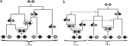Observe that associated with a randomly sampled ancestry is a sample configuration n with |n| = n specified haplotypes generated at the leaves. See Figure 1a for an illustration.

Figure 1.—

Illustrations of a genealogy and conditional genealogy for a two-locus (k = 2), two-allele model. The two loci of a haplotype are each represented by a circle, with the shading (light or dark) indicating the allelic type at that locus. Mutation events, along with the locus and resulting haplotype, are indicated by small arrows. Recombination events (always taking the left loci from the left side and the right locus from the right side), along with the resulting haplotype, are indicated by dotted circles. (a) A genealogy with n = 4. It is easy to verify that, starting with the MRCA and following the genealogy forward in time, the sample configuration n shown at the leaves is obtained. (b) An “observed” genealogy with n = 3 and a conditional genealogy with m = 1. Absorption events are indicated by dotted arrows into . Following the combined genealogy forward in time, it is easy to check that the conditional sample m shown at the leaf of is obtained.

Suppose we now wish to sample a collection of m additional haplotypes conditioned on having already observed a sample n and the true ancestry that generated n. The above-mentioned sampling scheme can be modified to sample a conditional ancestry relating a collection of m haplotypes to each other and to the sample n. As illustrated in Figure 1b, the conditional sampling scheme would comprise the usual genealogical events (mutation, recombination, and coalescence) involving the lineages in , along with coalescence events involving a lineage in and a lineage ancestral to n. We refer to the latter coalescence events as “absorption” events. Note that the ancestral lineages of the sample n completely determine the type of each lineage in involved in absorption events, and a valid conditional sample configuration m with |m| = m is generated at the leaves of .

There are three sources of complication to the approach just described: (1) The ancestry associated with a sample n is usually unknown; (2) although the genealogical process for is Markov, it is time inhomogeneous since the ancestry is nonconstant in time; and (3) if j lineages in survive till the time to the MRCA of , then one needs to simulate farther back in time with j + 1 lineages, conditioned on one of the lineages being the specified MRCA of . A genealogical approximation, resulting from the diffusion-generator technique described in the subsequent section, avoids all of these difficulties. 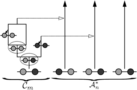Assume that , where is the nonrandom trunk ancestry defined as follows: Within , the lineages do not mutate, recombine, or coalesce with one another, and instead form a “trunk” extending infinitely into the past. See Figure 2 for an illustration. Note that is an improper ancestry, as there is no MRCA; nonetheless, the above conditional sampling procedure remains well defined. In particular, events within the conditional genealogy occur at the following rates:

• Mutation: Locus ℓ∈L of each lineage mutates with rate θ_ℓ/2.

• Recombination: Each lineage undergoes recombination about breakpoint b∈B with rate ρ_b/2.

• Coalescence: Each pair of lineages coalesces with rate 1.

• Absorption: Each lineage is absorbed into each lineage of with rate 1/2.

Figure 2.—

Illustration of a conditional genealogy using the approximation . Absorption events are indicated by dotted arrows into the “trunk” ancestry . Comparing with Figure 1b, observe that is time invariant and extends infinitely into the past.

Conversely, given a new sample m and a previously observed sample n, we may wish to compute the conditional sampling probability (CSP), denoted π(m | n). Although analytic computation of the CSP is impracticable for all but the smallest problems, using our genealogical approximation, namely that , it is possible to compute an approximate CSP by decomposing with respect to the unknown conditional genealogy . With denoting the probability of conditional ancestry , our approximation is

where if m is the configuration of haplotypes generated at the leaves of and 0 otherwise. Because is invariant in time, has a time-homogeneous Markov structure, and the above conditioning may be recast as a time-independent recursion. The solution thus obtained is our primary approximation, denoted . We next examine some computational aspects of and consider two genealogical approximations.

Computation and approximation:

There is no known general analytic formula for the recursion obtained for . The procedure for exact computation of , therefore, is to repeatedly invoke the recursion equation; this yields a closed set of coupled linear equations, which can be solved to provide the desired probability. It is instructive to quantify the size of the linear system that must be generated and solved. Suppose we are interested in the CSP of a single haplotype (i.e., |m| = 1); for simplicity, also assume that |E_ℓ| = s for all ℓ ∈ L. The number Q_k of equations produced for k loci is

where B_j is the jth Bell number, the number of partitions of a set of cardinality j into nonempty subsets. An algebraic identity involving the Bell numbers implies Q_k ≥ B_k+1 (with equality holding under a PIM model of mutation). Hence, since B_k+1 is superexponential in k, exact computation of is practicable only for k ≤ 12 loci. For k > 12, further approximations (or statistical techniques, which we do not further consider) are required. We describe below two approximations that together lead to an efficient algorithm. We later show empirically that the resulting CSDs have little loss of accuracy in comparison with .

Approximation 1 (disallowing coalescence):

Recall that a conditional genealogy is composed of mutation, recombination, coalescence, and absorption events. Importantly, within this framework, it is only coalescence events that can couple two lineages of into one (moving backward in time); mutation, recombination, and absorption events have the noncoupling effect of modifying, splitting, and removing lineages, respectively. Intuitively, then, by disallowing coalescence, separate lineages should behave independently; more precisely, given , and defining to be the CSP obtained from the genealogical process disallowing coalescence, we expect that

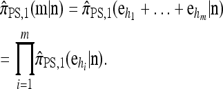(3)

This is indeed the case, as we prove in the next section. It is worth noting here that disallowing coalescence is not as unreasonable as it first may seem; unlike a normal genealogy, a conditional genealogy does not rely on coalescence events to terminate (absorption events play the analogous role). Although we shall further discuss the merit of this approximation in light of empirical results, for now, it suffices to say that (3) significantly simplifies computation of . Assuming a PIM model, a dynamic programming formulation of exists with asymptotic running time O(2^kk²) (for |m| = 1). Although still exponential in k, this represents a substantial improvement over , for which constructing and solving a system of equations superexponential in k is required.

Approximation 2 (limiting mutations):

We further examine , with the objective of finding a sensible polynomial time approximation. Even disallowing coalescence, it is necessary to consider every mutational configuration of the k loci. In a PIM model, there are O(2^k) such configurations, thereby accounting for the exponential running time given above. By artificially limiting the number of mutational configurations, it is again possible to substantially reduce the computational complexity.

In our final approximation , we limit the set of mutational configurations to those that are a single mutation away from the original haplotype. Genealogically, this corresponds to disallowing explicit mutation on any lineage that has already mutated; for small values of θ, we expect genealogies that do not conform to this restriction to be relatively unlikely. We shall further discuss the approximation in light of empirical results; for now, it suffices to remark that in a PIM model of mutation, is limited to k + 1 mutational states, enabling a modification to the dynamic program with asymptotic running time O(k³) (for |m| = 1). In principle, this allows the CSP to be computed for a number of loci k on the order of several hundred.

Relation to other approximate CSDs:

Several previously proposed approximate CSDs (Stephens and Donnelly 2000), (Fearnhead and Donnelly 2001), and (Li and Stephens 2003) are all naturally described as “copying” models, in which a new haplotype is conditionally sampled by making an imperfect copy of one or more haplotypes in an observed sample n. We now describe these copying models and show that each also has a genealogical interpretation; moreover, these interpretations can reasonably be described as approximations of our basic CSD, .

The copying model for , applicable when the loci are assumed completely linked (i.e., ρ = 0), is as follows: Select a random “source” haplotype h from n with probability n_h/n and a random copying time t from the exponential distribution with rate n/2; having done so, mutate each locus ℓ ∈ L of h a random number m_ℓ of times, with m_ℓ drawn from a Poisson distribution with mean θ_ℓt/2. The resulting haplotype is the conditional sample.

This copying model for can be restated as a genealogical process. In particular, set ρ = 0 and suppose we wish to conditionally sample a single haplotype. Both and are associated with a conditional genealogical process composed of the following events: mutation at locus ℓ ∈ L with rate θ_ℓ/2 and absorption into a haplotype lineage of n with rate 1/2. By the independence of the mutation and absorption events, this genealogical process coincides with the copying model for , suggesting that, when ρ = 0, . This is indeed the case, as we prove in the next section.

The approximate CSD extends to partially linked loci (i.e., ρ > 0). In this case, a new haplotype is sampled in two phases: First, an unspecified haplotype is randomly broken into unspecified fragments under the assumption that a break occurs at each b ∈ B independently and with probability ρ_b/(n + ρ_b); and second, each fragment is “copied” independently using the copying model, restricted to the appropriate set of loci. The specified fragments are then reassembled into a complete haplotype, completing the conditional sample. This copying model is often recast as a hidden Markov model (HMM), with observed states corresponding to the allele at each locus of the sampled haplotype, and hidden states corresponding to the source haplotype in n and copying time (as in the description of ); the probability of a transition in the hidden states is ρ_b/(n + ρ_b).

As in the case of , the copying model for can be restated as a genealogical process. In particular, consider the conditional genealogical process associated with , artificially divided into an initial “recombination phase,” wherein an unspecified haplotype is randomly broken into fragments, and a “non-recombination phase,” wherein these fragments are subject to the normal genealogical events, conditioned on no additional recombinations occurring. In the recombination phase, each breakpoint is used independently, and with probability ρ_b/(n + ρ_b), corresponding to the marginal probability of the breakpoint being used in the usual genealogical process for . In the nonrecombination phase, each fragment maintains independence by virtue of disallowing coalescence. This two-phase genealogical process coincides with the copying model for . We conclude that the approximate CSD can be considered an approximation of .

Finally, the approximate CSD is a computational simplification of in which the copying process for each fragment is assumed to have t = 2/n, rather than t drawn from an exponential distribution. This corresponds, in the associated genealogical process for , to the assumption that each fragment absorbed into some haplotype of n in time t = 2/n. We do not say anything further about since it is closely related to .

A MATHEMATICAL FORMULATION

In this section, we provide a mathematical derivation of our conditional sampling distribution. Rather than formalizing the genealogical interpretation/approximation discussed in the previous section, we extend the diffusion-generator approximation technique (De Iorio and Griffiths 2004a,b; Griffiths et al. 2008) and demonstrate equivalence. We also prove several useful limiting results and provide concrete mathematical statements for the approximations (disallowing coalescence and limiting mutations) mentioned in the previous section.

Notation:

To describe our mathematical formulation for an arbitrary number of loci, we need to introduce more notation. In what follows, we build on the notation defined in the previous section. Given a haplotype and a locus ℓ ∈ L = {1, …, k}, we use h[ℓ] ∈ E_ℓ to denote the allele at locus ℓ of h. Given any two haplotypes , we define the following operations:

• Substitute: Given a locus ℓ ∈ L and an allele a ∈ E_ℓ, define as the haplotype derived from h by substituting the allele at locus ℓ with a.

• Recombine: Given a breakpoint b = (ℓ, ℓ + 1) ∈ B, define as the mosaic haplotype derived by concatenating h[1], … , h[ℓ] and h′[ℓ + 1], … , h′[k].

We also require partially specified haplotypes, in which the alleles at some loci are unspecified. Denote such an unspecified allele by • and define the space of partially specified haplotypes as . For , let L(g) denote the set of loci at which g has specified (i.e., not •) alleles. Then, for , we say that g and g′ are compatible and write g ⋏ g′, if g[ℓ] = g′[ℓ] for all ℓ ∈ L(g)∩L(g′). We define an operation for combining two compatible partially specified haplotypes:

• Coalesce: If g ⋏ g′, define as the haplotype constructed as follows: For ℓ ∈ L, if g′[ℓ] = •, if g[ℓ] = •, and otherwise.

Given a partially specified haplotype , we use B(g) to denote the set of breakpoints between the leftmost and the rightmost loci in L(g) and define the following operation for breaking up g into parts:

• Break: Given a breakpoint b = (ℓ, ℓ + 1) ∈ B(g), we use to denote the haplotype obtained from g by replacing g[j] with • for all j ≥ ℓ + 1 and to denote the haplotype obtained from g by replacing g[j] with • for all j ≤ ℓ.

To illustrate the above definitions, consider a three-locus model, setting E_ℓ = {0, 1} for each locus ℓ ∈ L = {1, 2, 3}. Suppose g₁ = (•, •, 1), g₂ = (0, •, 1), and g₃ = (1, 1, •). The loci with specified alleles are L(g₁) = {3}, L(g₂) = {1, 3}, and L(g₃) = {1, 2}, and the valid breakpoints are B(g₁) = {Ø}, B(g₂) = {(1, 2), (2, 3)}, and B(g₃) = {(1, 2)}. Furthermore, g₁ ⋏ g₂ with •,1) and g₁ ⋏ g₃ with .

A general strategy for computing :

We begin by briefly reviewing the neutral multilocus diffusion process. Within this framework, we formally state the problem and outline the general strategy we use to solve it.

The neutral multilocus diffusion process:

Dual to the coalescent is a forward-in-time diffusion process. The state space of the multilocus diffusion process is

where x_h corresponds to the population-wide frequency of haplotype h. Being continuous in both time and space, diffusion processes possess many useful mathematical properties. In particular, associated with a diffusion process is a fundamental differential operator ℒ, called the generator, with the following property: For any bounded, twice-differentiable function f with continuous second derivatives, the generator satisfies ℰ[ℒf(X)] = 0, where ℰ denotes expectation with respect to the stationary distribution of the diffusion process. The diffusion generator for the neutral model with crossover recombination is ℒ=∑_h∈ℋℒ_h(∂/∂x_h), where

with δ_h,h′ denoting the Kronecker delta symbol. Denote by q(n) the probability of obtaining an ordered sample with configuration . Making reference to the diffusion process, q(n) = ℰ(q(n | X)), where q(n | X) is the conditional probability of obtaining n given the population frequencies ; more precisely, .

Now let with |m| = m. Denote by π(m | n) the conditional probability that, having already observed sample configuration n, the next m sampled haplotypes have configuration m. By the definition of conditional probability, the distributions π and q satisfy the following key identity:

(4)

The diffusion-generator formulation:

It is our objective to use the diffusion characterization of q(n) along with the above conditioning identity (4) to find a distribution approximating π. Shown below is an outline of the diffusion-generator approximation technique for computing :

1. At stationarity, instead of ℰ[ℒf(X)] = 0, assume that a distribution exists with expectation operator such that the vanishing condition holds componentwise; i.e., for each ,

   (5)

2. Define the approximate sampling distribution and, motivated by the conditioning identity (4), define the approximate CSD .

3. Use an appropriate set of functions f(X) and haplotypes in (5) to derive a recursion for that does not include terms.

Applying this general strategy, De Iorio and Griffiths (2004a,b) were able to reproduce formally the widely used one-locus CSD introduced by Stephens and Donnelly (2000); in a similar vein, Griffiths et al. (2008) were able to devise an approximate CSD in the case of two loci with a restricted mutation model. Our present goal is to apply this diffusion-generator formulation yet again to derive a recursion for an arbitrary number of loci and an arbitrary finite-alleles mutation model. This will be our approximate CSD, which we denote . After deriving the recursion for , we show that it coincides with the genealogical formulation of the previous section and provide some intuition for the above approximation.

The main recursion:

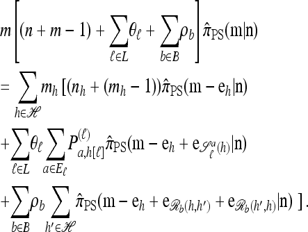
Using the diffusion-generator approximation formulation described above, we obtain the following theorem, which is proved in the appendix:

Theorem 1. Let with |m| = m and with |n| = n. Then the approximate conditional sampling distribution satisfies the following recursion:

(6)

Although we consider the recursion stated in Theorem 1 to be our primary result, explicit evaluation is not possible since the number of states that must be explored is infinite. To establish a practicable formulation, we extend this result to partially specified haplotypes.

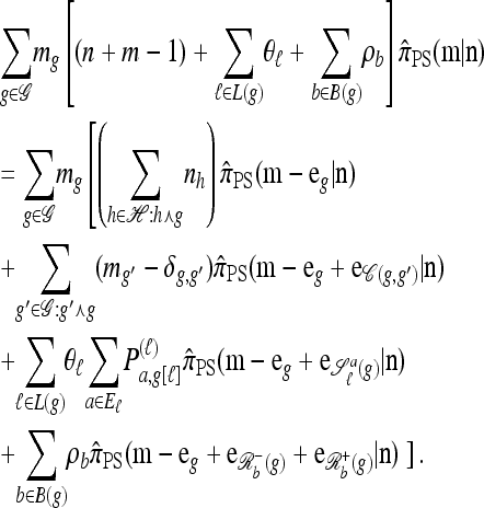
Suppose that is a configuration allowing unspecified alleles. Conditional on X, the sampling probability becomes , where is the total proportion of fully specified haplotypes that subsume the partially specified haplotype . With and defined as before with respect to and the above q(n | X), we obtain the following corollary (its proof is deferred to the appendix):

Corollary 2. Let with |m| = m and with |n| = n. Then the approximate conditional sampling distribution satisfies the following recursion:

(7)

Remark. Determining a simple recursion for in the general case, when (i.e., haplotypes in n may contain unspecified alleles), remains an important open problem.

To see that explicit evaluation is possible, suppose and and denote the total number of specified loci in m by . Applying (7) for , it is evident that each term on the right-hand side is of form with L(m′) ≤ L(m). Thus, by induction, only a finite number of states need be explored, and so repeated application of (7) yields a closed set of coupled linear equations, within which is a variable. This system can be solved using standard numerical techniques.

Connection to the genealogical formulation:

Recall the conditional genealogical process for constructing using the approximation described in the previous section. Employing this formulation, it is possible to compute by applying the law of total probability with respect to the most recent event (i.e., the usual “forward–backward” argument). We leave it to the reader to verify that doing so will yield the recursion (6) or (7), depending upon whether nonancestral loci are explicitly considered. This establishes the equivalence between our genealogical and mathematical formulations.

This equivalence may appear surprising given that the componentwise vanishing assumption (5) does not have an obvious genealogical interpretation. Griffiths et al. (2008) provide some intuition, pointing out that (5) is mathematically equivalent to assuming that, conditioning on sample n, the probability that the most recent event includes haplotype is equal to n_h/n. This is precisely the prior probability (i.e., the probability if the the haplotypes of n were unspecified) and therefore furnishes a reasonable and internally consistent approximation. Importantly, this assumption allows us to genealogically restrict attention to a particular haplotype h; we may thus restrict attention to the subconfiguration m of m + n. In this way, a genealogy that modifies only lineages associated with m is constructed, precisely what occurs in our genealogical formulation.

Analytic formulas:

In the one-locus case (k = 1) with parent-independent mutation, (7) immediately yields a conditional sampling formula that agrees with the exact one-locus CSD π. More precisely, given an additional allele and a previously observed sample with |n| = n, we obtain

(8)

Both Stephens and Donnelly (2000) and Fearnhead and Donnelly (2001) obtained the same result; as we shall soon see, this is part of a more general result that holds in the limit as ρ → 0.

In the two-locus case (k = 2) with parent-independent mutation, it is possible to obtain an analytic formula. Given an additional haplotype and a previously observed sample with |n| = n, we obtain

where , and π(e_a | n) is the exact one-locus CSP (8), with n appropriately marginalized. This form is quite similar to that derived by Griffiths et al. (2008), with the minor differences attributable to a different treatment of “symmetry” conditions.

Although it is theoretically possible to obtain analytic solutions for k > 2, little simplification is possible, and solving them is tantamount to generating and solving the coupled system of equations directly. We next show that some algebraic simplification is possible in two limiting cases.

Limiting distributions:

For convenience, we set ρ_b = ρ, for all b ∈ B, and consider the CSD in both the and the limits. We find that, in the limit, coincides with Stephens and Donnelly's CSD and, by extension, Fearnhead and Donnelly's . In the limit, coincides with , with in the case of parent-independent mutation.

The limit:

Set ρ = 0, and let m = e_h′ for some and . Then (6) yields the following simplified recursion:

(9)

Recall that Stephens and Donnelly's CSD , applicable when the loci are completely linked (i.e., ρ = 0), is formulated most naturally as a copying model, in which a new haplotype is conditionally sampled by choosing a previously sampled haplotype and stochastically mutating it according to a specified process (see the appendix for details). Despite the disparity of the genealogical description for and the copying model description for , the following proposition (also proved in the appendix) assures us that they are equivalent.

Proposition 3. Let m = e_h′ for some and . Then if ρ_b = 0 for all b ∈ B, .

In addition to providing a genealogical interpretation for , the above proposition indicates that, when ρ = 0, may be approximated using the Gaussian quadrature method proposed by Stephens and Donnelly (2000); conversely it provides an exact method for computing , generalizing similar results to an arbitrary number of loci and mutation model. Finally, when ρ = 0, Fearnhead and Donnelly's CSD coincides, by construction, with , and so .

The limit:

Let and denote the one-locus marginal configuration for ℓ ∈ L by , where is the number of haplotypes of n with allele a at locus ℓ. In the appendix, we prove that in the ρ → ∞ limit, may be decomposed into a product of one-locus likelihoods:

Proposition 4. Let and . Then in the limit ρ → ∞,

(10)

Recall that Fearnhead and Donnelly's CSD enjoys the same limiting decomposition, and the one-locus coincides with the one-locus , which in turn agrees with the one-locus by Proposition 3. In conjunction with Proposition 4, these facts imply that in the limit . It is encouraging that the true CSD π also exhibits this limiting decomposition (this follows directly from the well-known limiting decomposition of the sampling distribution q). Coupled with the fact that the one-locus CSD (8) is exact for PIM models, we may also conclude that for PIM models in the ρ → ∞ limit, .

Approximations to :

In the general case, when 0 < ρ < ∞, computing a CSP using requires that a set of coupled linear equations be constructed and solved. In particular, for |m| = 1 in the case of a PIM model, the number of generated equations is the (k + 1)th Bell number B_k+1, where k is the number of loci. Thus, the number of equations is superexponential in k, indicating that computation of is intractable with increasing k. We consider two approximations, motivated by the genealogical formulation discussed in the previous section.

Approximation 1 (disallowing coalescence):

Modifying (7) by disallowing coalescence—corresponding to removing the second term on the right-hand side and renormalizing the left-hand side—we obtain a recursion for a new approximate CSD, which we denote . Some genealogical justification for this approximation was provided for this in the previous section, and empirical justification is provided in the next section. Here, we are interested primarily in the computational aspects, which rely on the following result (proved in the appendix):

Proposition 5. For , where , and , the approximate CSD satisfies

(11)

Resulting from Proposition 5 is a simplified recursion for : Letting ,

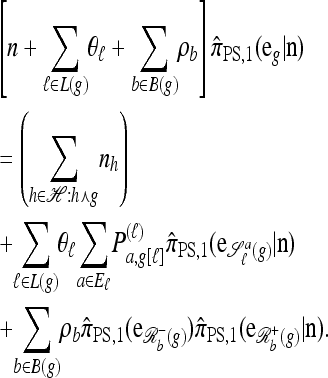(12)

Making use of this recursion, and assuming that |E_ℓ| = s for all ℓ ∈ L, a system of O(s^kk²) equations needs to be generated and solved, far fewer than the superexponential number required for . Moreover, assuming a PIM model of mutation, there is an evident dynamic programming formulation for that runs in O(2^k·k²) time.

Approximation 2 (limiting mutations):

Despite being significantly faster to compute than , the approximate CSD is still exponential in the number of loci. This remains true even for ρ = 0, indicating that the complication is a result of mutation rather than recombination. In particular, looking at the form of (12), it is clear that must be evaluated for every partially specified haplotype . As discussed in the previous section and empirically justified in the next section, when θ is relatively small, a reasonable approximation to may be obtained by artificially limiting the set of accessible haplotypes.

In particular, denote by the approximate CSD obtained by limiting the “explicitly computed” terms to those haplotypes that are within a single mutational step of the haplotype g of interest. Then,

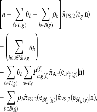(13)

where is an alternative approximate CSD. The “canonical” choice for is

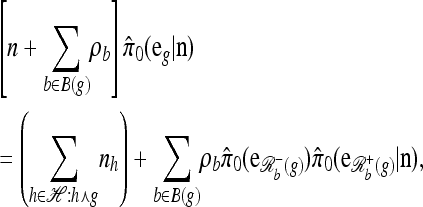which is (13) with further mutation disallowed (i.e., θ_ℓ = 0 for all ℓ ∈ L). Using , and again assuming that |E_ℓ| = s for all ℓ ∈ L, a system of O(sk³) equations needs to be generated and solved. Further assuming a PIM model of mutation, a dynamic programming formulation can be used, which runs in O(k³) time. We have found that better results are obtained by using , which implicitly does allow for additional mutation. This modification does not change the asymptotic running time.

EMPIRICAL RESULTS

In this section, we evaluate the accuracy of our CSD , along with the approximations and , and compare it with the accuracy of the approximate CSDs and , respectively proposed by Fearnhead and Donnelly (2001) and by Li and Stephens (2003). Analytically computing the true CSP is typically not possible, so we rely on importance sampling to provide reference values. Even within this Monte Carlo framework, the size of problems that can be analyzed is modest, thus limiting the scope of our study.

We find that and the associated approximations ( and ) are more accurate than and in a variety of circumstances. In addition, we consider the PAC pseudolikelihood framework mentioned in the Introduction and demonstrate that the improved accuracy of our CSDs has a positive impact on PAC-based estimation, generally providing improved accuracy for both likelihood and maximum-likelihood estimates.

Data simulation:

For simplicity, we consider a two-allele model and set and θ_ℓ = θ for all loci ℓ ∈ L and ρ_b = ρ for all breakpoints b ∈ B. Using a coalescent with recombination simulator, with ρ = ρ₀ and θ = θ₀, we may sample a k-locus n-haplotype sample configuration n. Given such a configuration, we may subsample a k′-locus n′-haplotype configuration n′ (for k′ ≤ k and n′ ≤ n) by randomly selecting n′ haplotypes and restricting attention to a k′ subset of the loci. In particular, the k′ subset is chosen as follows (method, M):

• M1. The central k′ loci, when θ₀ is large so that most or all loci segregate.

• M2. The central k′ segregating loci, when θ₀ is small so that few loci segregate. This procedure corresponds to the typical usage of on genomic data, in which only segregating sites are considered.

Finally, given a k-locus n-haplotype configuration n, we may subsample a k-locus n-haplotype conditional configuration C = (e_h, n − e_h) by withholding a single haplotype h from n uniformly at random. For notational simplicity, we define π on such a conditional configuration in the natural way: π_ρ(C) = π(e_h | n − e_h, ρ).

CSD accuracy:

We evaluate the accuracy of each approximate CSD as a function of three parameter values: the number of loci, k; the number of haplotypes in the conditional configuration, n; and the recombination rate, ρ. More precisely, we approximate the expected relative error as

(14)

where N denotes the number of simulated data sets and C⁽ⁱ⁾ is a k-locus n-haplotype conditional configuration sampled as indicated above, with parameters θ₀ and ρ₀. To keep the requisite computation reasonable, we consider three experiments, each time fixing two parameters and allowing the third one to vary. In all cases, θ = θ₀ is used to evaluate . The results for and are very similar, so below we discuss only the latter.

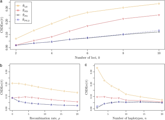
We first consider the case in which θ₀ = 1 and ρ₀ = 4. Biologically θ₀ = 1 corresponds to a relatively high mutation rate, not so uncommon in retroviruses (McVean et al. 2002). The specific parameter settings and results are shown in Figure 3. Under these circumstances, the CSDErr values of our approximations and are comparable and are smaller than those for both and . We remark that these are averaged results and do not imply that the CSP produced by is always more accurate than that produced by or .

Figure 3.—

Relative error of CSDs for θ₀ = 1 and ρ₀ = 4. See (14) for definition of . With θ₀ = 1 and ρ₀ = 4, we used a coalescent simulator to generate 250 data sets, each with 25 haplotypes and 10 loci. Then, requisite k-locus, n-haplotype conditional configurations {C⁽ⁱ⁾}_{i=1, …, 250} were obtained using method M1 described in the text. (a) k ∈ {2, 3, 4, 5, 6, 8, 10}, n = 6, and ρ = ρ₀. (b) k = 4, n = 6, and ρ ∈ {0, 2, 4, 6, 8, 12, 16, 20}. (c) k = 4, n ∈ {2, 4, 6, 8, 10, 14, 20}, and ρ = ρ₀.

All of the approximate CSDs become less accurate as the number of loci increases (see Figure 3a). However, there is significant variation in the rate that this loss occurs, and and lose accuracy more quickly than and ; this result may have a significant consequence at a genomic scale, in which hundreds of segregating loci (or many more) are often considered. In contrast, all of the approximate CSDs become more accurate as the recombination rate increases (see Figure 3b). The correspondence between and at ρ = 0 may be explained by the theoretical result in Proposition 3 and the surrounding discussion; similarly, Proposition 4 ensures that in the ρ → ∞ limit, indicating that the values of CSDErr for , , and converge to 0. Finally, as the number of haplotypes in the conditional configuration increases, the values of CSDErr for the different CSDs appear to converge (see Figure 3c). Interestingly, as the number n of haplotypes decreases, becomes less accurate, while becomes more accurate; this result may have an effect on PAC computation, since small conditional configurations are necessarily considered.

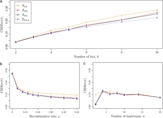
We next consider the case in which θ₀ = 0.01 and ρ₀ = 0.1, corresponding biologically to moderate mutation and recombination rates. The specific parameter settings and results are presented in Figure 4. As in the previous case, the approximations and are generally more accurate than and . The accuracy differences among the approximations, however, are less pronounced; the precise cause and degree of this effect (as the parameters, including θ₀ and ρ₀, vary) require further theoretical and empirical investigation.

Figure 4.—

Relative error of CSDs for θ₀ = 0.01 and ρ₀ = 0.1. See (14) for definition of . With θ₀ = 0.01 and ρ₀ = 0.1, we used a coalescent simulator to generate 250 data sets, each with 25 haplotypes and 500 loci. Then, requisite k-locus n-haplotype conditional configurations {C⁽ⁱ⁾}_{i=1, …, 250} were obtained using method M2 described in the text. (a) k ∈ {2, 3, 4, 5, 6, 8, 10}, n = 6, and ρ = ρ₀. (b) k = 4, n = 6, and ρ ∈ {0, 4, 8, 12, 16, 20, 30, 40, 50} × 10⁻². (c) k = 4, n ∈ {2, 4, 6, 8, 10, 14, 20}, and ρ = ρ₀.

As before, all of the CSDs become less accurate as the number of loci increases (see Figure 4a) and more accurate as the recombination rate increases (see Figure 4b). In contrast with the previous case, appears to be somewhat more accurate than ; this result is surprising since makes more approximations than . A similar phenomenon appears in the context of PAC accuracy and is explored in more detail below. Finally, as the number of haplotypes in the conditional configuration increases, the values of CSDErr for the different CSDs appear to converge (see Figure 4c); as before, for small numbers of haplotypes is less accurate than , although the difference is less pronounced.

PAC-likelihood accuracy:

We evaluate the accuracy of each approximate CSD in the context of the PAC pseudolikelihood framework. Since the true CSD π provides the correct likelihood within this framework, we expect that better approximations provide better approximations of the true likelihood. Denote by the ordered PAC likelihood obtained using CSD and 100 random permutations of the haplotypes in n. We approximate the mean relative error as

(15)

where N denotes the number of simulated data sets and n⁽ⁱ⁾ is a k-locus n-haplotype configuration sampled from the coalescent with recombination, with parameters θ₀ and ρ₀. We consider fixing k and n and allowing ρ to vary. In all cases, θ = θ₀ is used to evaluate . The PAC-likelihood accuracy results for and are very similar, and so below we discuss only the latter.

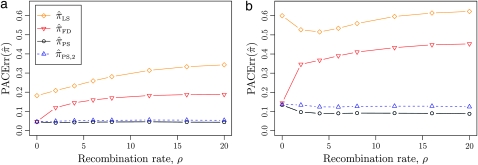
We first consider the case in which θ₀ = 1 and ρ₀ = 4. The specific parameter settings and results are presented in Figure 5. Under these circumstances, the approximations and yield PAC likelihoods that are more accurate than those produced using or . Moreover, comparing Figure 5a and 5b for k = 3 and k = 5 loci, respectively, it appears that as the number of loci increases, the difference in PAC-likelihood accuracy increases; this result might be anticipated from Figure 3a, which shows that the difference in CSD accuracy increases in a similar fashion. Finally, for the range of recombination rates shown, observe that PACErr for and notably increases as ρ increases; PACErr for also increases as ρ increases, but only slightly. Contrast this with Figure 3b, which shows that the CSD accuracy decreases as the recombination rate increases. This result is particularly surprising since PACErr → 0 for both and (because ) in the ρ → ∞ limit.

Figure 5.—

Relative error of PAC likelihoods for θ₀ = 1 and ρ₀ = 4. See (15) for definition of . With θ₀ = 1 and ρ₀ = 4, we used a coalescent simulator to generate 250 data sets, each with 25 haplotypes and 10 loci. Then, requisite k-locus n-haplotype configurations {n⁽ⁱ⁾}_{i=1, …, 250} were obtained using method M1 described in the text. (a) k = 3, n = 25, and ρ ∈ {0, 2, 4, 6, 8, 12, 16, 20}. (b) k = 5, n = 25, and ρ ∈ {0, 2, 4, 6, 8, 12, 16, 20}.

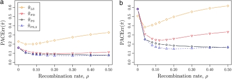
We next consider the case in which θ₀ = 0.01 and ρ₀ = 0.1. The specific parameter settings and results are presented in Figure 6. As before, the approximations and yield PAC likelihoods that are more accurate than those produced using and , and this effect appears to increase with the number of loci. Comparing with CSDErr in Figure 4, there are two interesting observations: First, in contrast to the similar values of CSDErr for and , the PAC likelihoods using are significantly more accurate than those using ; and second, in concordance with the smaller values of CSDErr for than for , the PAC likelihoods using are more accurate than those using for much of the domain.

Figure 6.—

Relative error of PAC likelihoods for θ₀ = 0.01 and ρ₀ = 0.1. See (15) for definition of . With θ₀ = 0.01 and ρ₀ = 0.1, we used a coalescent simulator to generate 250 data sets, each with 25 haplotypes and 500 loci. Then, requisite k-locus n-haplotype configurations {n⁽ⁱ⁾}_{i=1, …, 250} were obtained using method M2 described in the text. (a) k = 3, n = 25, and ρ ∈ {0, 4, 8, 12, 16, 20, 30, 40, 50} × 10⁻². (b) k = 5, n = 25, and ρ ∈ {0, 4, 8, 12, 16, 20, 30, 40, 50} × 10⁻².

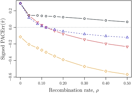
Thus motivated, we consider the signed PACErr, obtained by removing the absolute value from (15); the signed result corresponding to Figure 6b is presented in Figure 7. Observe that the values of the signed PACErr for both and are initially positive, pass through 0 to become negative, and ultimately must return to 0 in the ρ → ∞ limit; in contrast, values of the signed PACErr for make a more deliberate descent toward 0. We might expect that such “transient” domains of near unbiasedness demonstrated by and affect the accuracy of the associated PACErr.

Figure 7.—

Approximate values of signed PACErr for θ₀ = 0.01 and ρ₀ = 0.1, corresponding to Figure 6b. The correspondence between the symbols and 's is the same as in previous figures.

Indeed, comparing with Figure 6b, there is a rough correspondence between the domains in which values of the signed PACErr for and are very near 0 and the domains in which the PAC likelihoods using and have the highest accuracy. Within these respective domains, produces a PAC likelihood that is more accurate than , but does not, an effect that may be due to an increased variance associated with . Finally, recall that is also more accurate than in terms of CSDErr (see Figure 4). A comparable analysis of signed CSDErr (data not shown) indicates that a similar effect may be at work, although on a significantly larger scale; additional results would need to be collected to make this claim decisively.

PAC–maximum-likelihood estimate accuracy:

Finally, we consider using the PAC pseudolikelihood framework to obtain maximum-likelihood estimates (MLEs) for the recombination rate ρ. Since the true CSD π would provide the true MLE within this framework, we expect that better approximations will provide better MLEs. Denote by the PAC–MLE obtained using a golden section search on the PAC-likelihood surface associated with the CSD and 100 random permutations of the haplotypes in n.

Following Li and Stephens (2003), we compute the per-n error , where ρ₀ is the recombination rate under which the n was generated. Note that indicates that ; although this is ostensibly a good property, we note here that the true MLE does not satisfy this property in expectation and may not satisfy it in median. In keeping with our previous empirical results, we believe that a more important comparison is directly between and . Unfortunately, such comparisons are difficult for two reasons: First, can take the values 0 and ∞, making comparisons with difficult; and second, is difficult to compute.

With this caveat in mind, we continue with Li and Stephens' formulation. Treating n as a random variable, compute the sample median and interquartile range (IQR) of the distribution associated with . The specific parameter settings used and results are presented in Table 1. Observe that, as the number of loci increases, the IQR generally becomes smaller, indicating that the distribution is becoming more concentrated about the median. In the case that θ₀ = 1 and ρ₀ = 4, the results are promising; the approximations , , and have medians significantly nearer to 0 than and . Moreover, this effect becomes more pronounced as the number of loci increases. The results are less clear in the θ₀ = 0.01 and ρ₀ = 0.1 case. All of the CSDs demonstrate comparable medians, none particularly close to 0; as the number of loci increases, there appears to be some trend toward a median of 0 for all CSDs. Once again, we urge caution in interpreting these results, as the nature of the true distribution Err_π(n) remains unknown.

TABLE 1.

PAC-maximum-likelihood estimate accuracy

	θ0 = 1, ρ0 = 4						θ0 = 0.01, ρ0 = 0.1
	k = 5		k = 7		k = 9		k = 5		k = 7		k = 9
	Median	IQR	Median	IQR	Median	IQR	Median	IQR	Median	IQR	Median	IQR
	−0.07	3.57	—	—	—	—	−0.74	3.01	—	—	—	—
	−0.19	3.58	+0.10	2.05	+0.05	1.64	−0.94	3.14	−0.94	2.14	−0.80	1.55
	−0.39	3.75	−0.11	2.17	−0.22	1.79	−0.94	3.10	−0.94	2.14	−0.82	1.58
	−0.79	3.98	−0.80	2.19	−0.96	1.70	−0.99	3.01	−1.00	2.02	−0.87	1.49
	−1.02	4.58	−0.91	2.33	−1.19	1.86	−0.83	3.15	−0.85	1.88	−0.68	1.23

Median and interquartile range (IQR) estimates for the distribution Err_π̂(n) = log₂[ρ_π̂(n)/ρ₀]. Estimates are computed using 250 k-locus 25-haplotype configurations generated from a coalescence simulator using θ₀ and ρ₀.

DISCUSSION

In this article, we generalized the diffusion-generator approximation technique to derive a novel approximate conditional sampling distribution, , for an arbitrary number of loci and an arbitrary finite-alleles recurrent mutation model. Furthermore, we described a genealogical interpretation for on the basis of the idea of conditional genealogies. In addition to providing intuition for the mathematical techniques used to derive , the genealogical interpretation motivated us to introduce additional approximations that reduce the asymptotic time complexity of our from superexponential in k (the number of loci) to cubic in k. We observed that the approximation of disallowing coalescence in the conditional genealogy works remarkably well, leading to little loss in accuracy compared with . We note that this is probably because the empirical study we carried out is for the case in which the haplotypes in the conditional sample configuration m have pairwise disjoint sets of specified alleles. For a more general sample m, we suspect that disallowing coalescence in may not work as well. Incidentally, note that disallowing coalescence between haplotypes with no overlapping specified alleles is closely related to the so-called sequentially Markov coalescent (McVean and Cardin 2005; Marjoram and Wall 2006; Chen et al. 2009), an approximation to the full sequential coalescent formulation introduced by Wiuf and Hein (1999).

In our empirical study, we found that our CSD and the associated approximations ( and ) are in general more accurate than the previously proposed CSDs. Importantly, this improvement in accuracy gets amplified as the number of loci increases. Moreover, the improvement in CSD accuracy carries over to the PAC framework, for both PAC-likelihood estimation and, to a lesser extent, PAC–MLE estimation. Interestingly, as the mutation rate θ decreases, some improvements in accuracy are attenuated, while others are not. We believe that studying and understanding these effects is an important future research direction.

Approximate CSDs have been fruitfully used in Monte Carlo techniques (e.g., importance sampling) and other approximation strategies (typically via the PAC approximation). In principle, our new CSD may be applied in many of the same situations, potentially providing improved efficiency in the Monte Carlo setting and improved accuracy in the approximation setting. In practice, the details of many algorithms explicitly depend on the CSD used, so we leave as future research adapting such algorithms to the form of . We believe that the work discussed here will have several useful applications in both computational biology and population genetics analysis.

APPENDIX

Proof of Theorem 1. By the componentwise vanishing property (5), for any bounded, twice-differentiable function f with continuous second derivatives,

Setting f(x) = q(n | x) implies the following relation for :

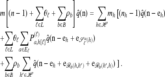Substituting and, recalling (4), dividing by produces (6), thereby completing the proof. ▪

Proof of Corollary 2. This result follows from Theorem 1. Without loss of generality, let for and . Recalling (4) and the appropriate definitions,

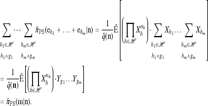(A1)

Substituting for into (6),

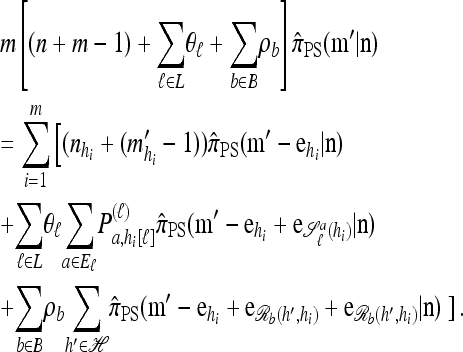(A2)

Applying (A1) to the left-hand side of (A2) and doing some algebraic manipulation,

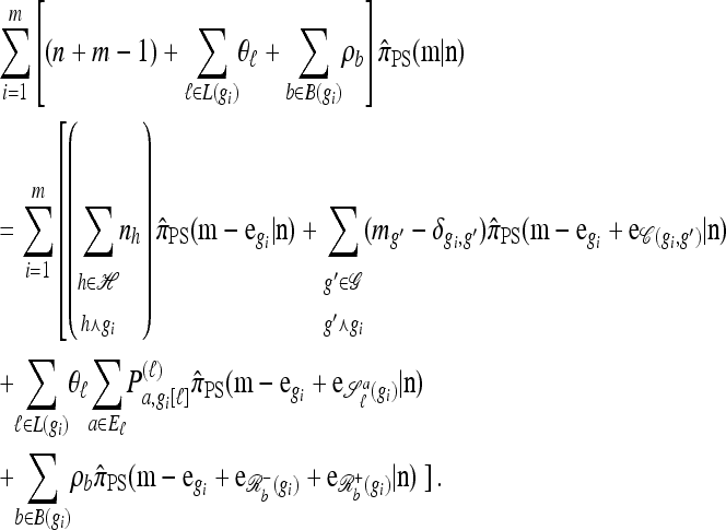This result is equivalent to (7), completing the proof. ▪

Proof of Proposition 3. Let be an observed haplotype configuration. Stephens and Donnelly's CSD is formulated by assuming that a new haplotype may be conditionally sampled by choosing a haplotype from n uniformly at random and mutating the loci using a prescribed scheme dependent on θ_ℓ and P^(ℓ) = (P) for each locus ℓ ∈ L. Letting ,

(A3)

where s = (s₁, …, s_m) denotes the number of mutations at each locus, , is the multinomial coefficient, and F(h, h′, s) is the probability of h mutating to h′ with s_ℓ mutations at each locus ℓ ∈ L,

where . We show that obeys the same recursion as . By removing the summand with s = 0 ∈ N^m in Equation A3, we obtain

(A4)

Additionally, we have that F(h, h′, 0) = δ_h,h′/(n + Θ), and

Substituting these identities into (A4) yields the recursion

which is identical to the recursion (9) for , thereby proving the proposition. ▪

Proof of Proposition 4. Define as the total number of valid breakpoints in m. Using (7) in the limit that and assuming B(m) > 0,

Repeated application of this equation yields the key identity

(A5)

where m* is derived from m by recombination at every possible breakpoint. More precisely, define to be the haplotype with allele a ∈ E_ℓ at locus ℓ ∈ L and · elsewhere. Then

Observing that B(m*) = 0, we may apply (A5) to (7) to obtain

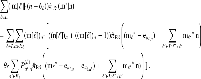(A6)

Observe that (A6) is a sum of independent recursions, each for a particular locus ℓ ∈ L. It is thus easily verified that the recursion has solution

In conjunction with (A5), this produces the desired result. ▪

Proof of Proposition 5. As described, the is the approximate CSD obtained by removing the second term on the right-hand side of (7) and renormalizing the left-hand side. Writing the resulting recursion for ,

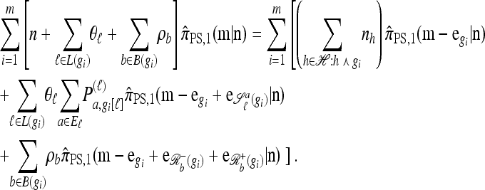(A7)

Observe that (A7) is a sum of independent recursions, each for a particular haplotype . It is thus easily verified that the recursion has solution

which is our desired result. ▪

References

- Chen, G. K., P. Marjoram and J. D. Wall, 2009. Fast and flexible simulation of DNA sequence data. Genome Res. 19 136–142. [DOI] [PMC free article] [PubMed] [Google Scholar]
- Crawford, D. C., T. Bhangale, N. Li, G. Hellenthal, M. J. Rieder et al., 2004. Evidence for substantial fine-scale variation in recombination rates across the human genome. Nat. Genet. 36 700–706. [DOI] [PubMed] [Google Scholar]
- Davison, D., J. K. Pritchard and G. Coop, 2009. An approximate likelihood for genetic data under a model with recombination and population splitting. Theor. Popul. Biol. 75(4): 331–345. [DOI] [PMC free article] [PubMed] [Google Scholar]
- De Iorio, M., and R. C. Griffiths, 2004. a Importance sampling on coalescent histories I. Adv. Appl. Probab. 36 417–433. [Google Scholar]
- De Iorio, M., and R. C. Griffiths, 2004. b Importance sampling on coalescent histories II. Adv. Appl. Probab. 36 434–454. [Google Scholar]
- Fearnhead, P., and P. Donnelly, 2001. Estimating recombination rates from population genetic data. Genetics 159 1299–1318. [DOI] [PMC free article] [PubMed] [Google Scholar]
- Fearnhead, P., and P. Donnelly, 2002. Approximate likelihood methods for estimating local recombination rates. J. R. Stat. Soc. B 64 657–680. [Google Scholar]
- Fearnhead, P., and N. G. C. Smith, 2005. A novel method with improved power to detect recombination hotspots from polymorphism data reveals multiple hotspots in human genes. Am. J. Hum. Genet. 77 781–794. [DOI] [PMC free article] [PubMed] [Google Scholar]
- Gay, J. C., S. Myers and G. McVean, 2007. Estimating meiotic gene conversion rates from population genetic data. Genetics 177 881–894. [DOI] [PMC free article] [PubMed] [Google Scholar]
- Griffiths, R. C., 1981. Neutral two-locus multiple allele models with recombination. Theor. Popul. Biol. 19 169–186. [Google Scholar]
- Griffiths, R. C., and P. Marjoram, 1996. Ancestral inference from samples of DNA sequences with recombination. J. Comput. Biol. 3(4): 479–502. [DOI] [PubMed] [Google Scholar]
- Griffiths, R. C., P. A. Jenkins and Y. S. Song, 2008. Importance sampling and the two-locus model with subdivided population structure. Adv. Appl. Probab. 40(2): 473–500. [DOI] [PMC free article] [PubMed] [Google Scholar]
- Hellenthal, G., A. Auton and D. Falush, 2008. Inferring human colonization history using a copying model. PLoS Genet. 4 e1000078. [DOI] [PMC free article] [PubMed] [Google Scholar]
- Howie, B. N., P. Donnelly and J. Marchini, 2009. A flexible and accurate genotype imputation method for the next generation of genome-wide association studies. PLoS Genet. 5(6): e1000529. [DOI] [PMC free article] [PubMed] [Google Scholar]
- Hudson, R. R., 1983. Properties of a neutral allele model with intragenic recombination. Theor. Popul. Biol. 23 183–201. [DOI] [PubMed] [Google Scholar]
- Hudson, R. R., 2001. Two-locus sampling distributions and their application. Genetics 159 1805–1817. [DOI] [PMC free article] [PubMed] [Google Scholar]
- Jenkins, P. A., and Y. S. Song, 2009. Closed-form two-locus sampling distributions: accuracy and universality. Genetics 183 1087–1103. [DOI] [PMC free article] [PubMed] [Google Scholar]
- Jenkins, P. A., and Y. S. Song, 2010. An asymptotic sampling formula for the coalescent with recombination. Ann. Appl. Probab. 20 1005–1028. [DOI] [PMC free article] [PubMed] [Google Scholar]
- Johnson, P., and M. Slatkin, 2009. Inference of microbial recombination rates from metagenomic data. PLoS Genet. 5(10): e1000674. [DOI] [PMC free article] [PubMed] [Google Scholar]
- Kingman, J. F. C., 1982. a The coalescent. Stoch. Proc. Appl. 13 235–248. [Google Scholar]
- Kingman, J. F. C., 1982. b On the genealogy of large populations. J. Appl. Probab. 19A 27–43. [Google Scholar]
- Kuhner, M. K., J. Yamato and J. Felsenstein, 2000. Maximum likelihood estimation of recombination rates from population data. Genetics 156 1393–1401. [DOI] [PMC free article] [PubMed] [Google Scholar]
- Li, N., and M. Stephens, 2003. Modeling linkage disequilibrium and identifying recombination hotspots using single-nucleotide polymorphism data. Genetics 165 2213–2233. [DOI] [PMC free article] [PubMed] [Google Scholar]
- Li, Y., and G. R. Abecasis, 2006. Mach 1.0: rapid haplotype reconstruction and missing genotype inference. Am. J. Hum. Genet. S79 2290. [Google Scholar]
- Marchini, J., B. Howie, S. R. Myers, G. McVean and P. Donnelly, 2007. A new multipoint method for genome-wide association studies by imputation of genotypes. Nat. Genet. 39(7): 906–913. [DOI] [PubMed] [Google Scholar]
- Marjoram, P., and S. Tavaré, 2006. Modern computational approaches for analysing molecular genetic variation data. Nat. Rev. Genet. 7 759–770. [DOI] [PubMed] [Google Scholar]
- Marjoram, P., and J. D. Wall, 2006. Fast “coalescent” simulation. BMC Genet. 7 16. [DOI] [PMC free article] [PubMed] [Google Scholar]
- McVean, G., and N. Cardin, 2005. Approximating the coalescent with recombination. Philos. Trans. R. Soc. Lond. B Biol. Sci. 360 1387–1393. [DOI] [PMC free article] [PubMed] [Google Scholar]
- McVean, G., P. Awadalla and P. Fearnhead, 2002. A coalescent-based method for detecting and estimating recombination from gene sequences. Genetics 160 1231–1241. [DOI] [PMC free article] [PubMed] [Google Scholar]
- McVean, G. A. T., S. R. Myers, S. Hunt, P. Deloukas, D. R. Bentley et al., 2004. The fine-scale structure of recombination rate variation in the human genome. Science 304 581–584. [DOI] [PubMed] [Google Scholar]
- Nielsen, R., 2000. Estimation of population parameters and recombination rates from single nucleotide polymorphisms. Genetics 154 931–942. [DOI] [PMC free article] [PubMed] [Google Scholar]
- Price, A. L., A. Tandon, N. Patterson, K. C. Barnes, N. Rafaels et al., 2009. Sensitive detection of chromosomal segments of distinct ancestry in admixed populations. PLoS Genet. 5(6): e1000519. [DOI] [PMC free article] [PubMed] [Google Scholar]
- Scheet, P., and M. Stephens, 2006. A fast and flexible statistical model for large-scale population genotype data: applications to inferring missing genotypes and haplotypic phase. Am. J. Hum. Genet. 78 629–644. [DOI] [PMC free article] [PubMed] [Google Scholar]
- Stephens, M., and P. Donnelly, 2000. Inference in molecular population genetics. J. R. Stat. Soc. B 62 605–655. [Google Scholar]
- Stephens, M., and P. Scheet, 2005. Accounting for decay of linkage disequilibrium in haplotype inference and missing-data imputation. Am. J. Hum. Genet. 76(3): 449–462. [DOI] [PMC free article] [PubMed] [Google Scholar]
- Wang, Y., and B. Rannala, 2008. Bayesian inference of fine-scale recombination rates using population genomic data. Philos. Trans. R. Soc. B 363(1512): 3921–3930. [DOI] [PMC free article] [PubMed] [Google Scholar]
- Wiuf, C., and J. Hein, 1999. Recombination as a point process along sequences. Theor. Popul. Biol. 55(3): 248–259. [DOI] [PubMed] [Google Scholar]
- Yin, J., M. I. Jordan and Y. S. Song, 2009. Joint estimation of gene conversion rates and mean conversion tract lengths from population SNP data. Bioinformatics 25(12): i231–i239. [DOI] [PMC free article] [PubMed] [Google Scholar]