Limits of stereopsis explained by local cross-correlation

Abstract

Human stereopsis has two well-known constraints: the disparity-gradient limit, which is the inability to perceive depth when the change in disparity within a region is too large, and the limit of stereoresolution, which is the inability to perceive spatial variations in disparity that occur at too fine a spatial scale. We propose that both limitations can be understood as byproducts of estimating disparity by cross-correlating the two eyes’ images, the fundamental computation underlying the disparity-energy model. To test this proposal, we constructed a local cross-correlation model with biologically motivated properties. We then compared model and human behaviors in the same psychophysical tasks. The model and humans behaved quite similarly: they both exhibited a disparity-gradient limit and had similar stereoresolution thresholds. Performance was affected similarly by changes in a variety of stimulus parameters. By modeling the effects of stimulus blur and of using different sizes of image patches, we found evidence that the smallest neural mechanism humans use to estimate disparity is 3–6 arcmin in diameter. We conclude that the disparity-gradient limit and stereoresolution are indeed byproducts of using local cross-correlation to estimate disparity.

Introduction

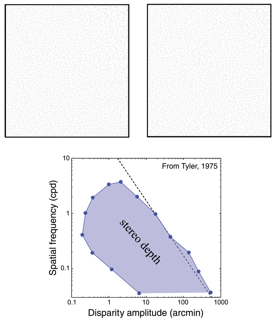
Stereopsis, the ability to perceive depth from binocular disparity, is limited by a number of factors. The variation in disparity from one part of the stimulus to another must be large enough to produce a discernible variation in perceived depth. This just-noticeable variation is the disparity threshold. But the magnitude of disparity variation must not be too great; otherwise, the two eyes’ images cannot be fused and the depth percept collapses. This maximum disparity is the fusion limit or D_max. Finally, the spatial variation in disparity from one part of the stimulus to another must not occur at too fine a scale. The finest perceptible variation is the stereoresolution limit. These limits to stereopsis are summarized in Figure 1. The upper panel is a stereogram of sinusoidal corrugations in which disparity amplitude increases from left to right and spatial frequency increases from bottom to top. View the stereogram at a distance of 40 cm and cross-fuse or divergently fuse to see the corrugations. One can perceive the sinusoidal depth variation in the middle of the stereogram but not elsewhere. The lower panel is a graph, replotted from Tyler (1975), showing the combinations of disparity amplitude and spatial frequency for which the corrugation in depth is perceived and the combinations for which it is not. Our purpose is to better understand the determinants of the boundary conditions for stereopsis.

Figure 1.

Combinations of disparity and spatial frequency that yield stereoscopic depth percepts. The upper panels are a stereogram that specifies sinusoidal depth corrugations. Cross fuse or divergently fuse to see the corrugations. Disparity amplitude increases from left to right and spatial frequency from bottom to top. The lower panel is replotted from Tyler (1975). The shaded region represents the combinations of disparity amplitude and spatial frequency that produce stereoscopic depth percepts: specifically, the ability to see the depth corrugation. The unshaded region represents combinations that do not yield such percepts. Along the dashed line, the product of spatial frequency and disparity is constant. The percept from the stereogram in the upper panel corresponds roughly to the graph in the lower panel if you view the stereogram from 40 cm.

To estimate disparity, the visual system must determine which parts of the two retinal images correspond. Doing this by cross-correlating the two eyes’ images has been used successfully in computer vision (Clerc & Mallat, 2002; Kanade & Okutomi, 1994), in modeling human vision (Banks, Gepshtein, & Landy, 2004; Cormack, Stevenson, & Schor, 1991; Fleet, Wagner, & Heeger, 1996; Harris, McKee, & Smallman, 1997), and in modeling binocular interaction in visual cortex. The prevailing model of binocular integration in visual cortex is the disparity-energy model (Cumming & DeAngelis, 2001; Ohzawa, 1998; Ohzawa, DeAngelis, & Freeman, 1990). In this model, the output of binocular complex cells can be expressed as

$$C(X_{\mathrm{L}},X_{\mathrm{R}})={(S_{\mathrm{L}}^{\text{even}})}^2+{(S_{\mathrm{L}}^{\text{odd}})}^2+{(S_{\mathrm{R}}^{\text{even}})}^2+{(S_{\mathrm{L}}^{\text{odd}})}^2+2S_{\mathrm{L}}^{\text{even}}{S}_{\mathrm{R}}^{\text{even}}+2S_{\mathrm{L}}^{\text{odd}}{S}_{\mathrm{R}}^{\text{odd}},$$ (1)

where S_L,R are the responses of simple cells in the left and right eyes and even and odd refer to the symmetry of the simple-cell receptive fields (Prince & Eagle, 2000). In the last two terms, the left eye’s response is multiplied by the right eye’s response. A bank of such cells, each tuned for a different disparity, making this computation performs the equivalent of windowed or local cross-correlation.

In this paper, we investigate whether the limits of stereopsis revealed in Figure 1 are byproducts of using local cross-correlation to estimate disparity from the two eyes’ images. To do so, we construct a local cross-correlator with biologically motivated properties and compare its behavior to that of human observers. In the first section, we consider the cause of the limit on the upper right side of the shaded area in Figure 1; we point out, as have Burt and Julesz (1980) and Tyler (1974, 1975), that the transition with increasing disparity from perceptible to imperceptible is well described by the disparity-gradient limit. By comparing human and model performances, we show that this limit is a byproduct of estimating disparity by correlation. In the second section, we consider the cause of the limit on the upper part of the shaded region in Figure 1. We again compare human and model performances and show that this stereoresolution limit is also a byproduct of estimating disparity by correlation.

The disparity-gradient limit

Sinusoidal corrugations in random-element stereograms cannot be discriminated when the product of corrugation spatial frequency and disparity amplitude exceeds a critical value (Tyler, 1974, 1975; Ziegler, Hess, & Kingdom, 2000). A similar phenomenon was observed by Burt and Julesz (1980) who reported that two-element stereograms cannot be fused when the angular separation between the elements is less than the disparity. Burt and Julesz argued that the limit to fusion is not disparity per se, as suggested by the notion of Panum’s fusional area (Panum, 1858). Rather the limit is a ratio: the separation divided by the disparity. This critical ratio is the disparity-gradient limit.

The disparity gradient is clearly defined for two-element stimuli. For elements P and Q in a stereogram, the coordinates in the left eye’s image are (x_PL, y_PL) and (x_QL, y_QL), and the coordinates in the right eye are (x_PR, y_PR) and (x_QR, y_QR). The separation is the vector S from the average position of P to the average position of Q. Its magnitude is

$$|\mathit{S}|=\sqrt{{\left[\frac{x_{\text{PL}}-x_{\text{QL}}+x_{\text{PR}}-x_{\text{QR}}}{2}\right]}^2+{\left[\frac{y_{\text{PL}}-y_{\text{QL}}+y_{\text{PR}}-y_{\text{QR}}}{2}\right]}^2},$$ (2)

and its direction is

$${\text{tan}}^{-1}\left[\frac{y_{\text{PL}}-y_{\text{QL}}+y_{\text{PR}}-y_{\text{QR}}}{x_{\text{PL}}-x_{\text{QL}}+x_{\text{PR}}-x_{\text{QR}}}\right].$$ (3)

The disparity is the vector D; its magnitude is

$$|\mathit{D}|=\sqrt{{[x_{\text{PL}}-x_{\text{QL}}+x_{\text{QR}}-x_{\text{PR}}]}^2+{[y_{\text{PL}}-y_{\text{QL}}+y_{\text{QR}}-y_{\text{PR}}]}^2},$$ (4)

and its direction is

$${\text{tan}}^{-1}\left[\frac{y_{\text{PL}}-y_{\text{QL}}+y_{\text{QR}}-y_{\text{PR}}}{x_{\text{PL}}-x_{\text{QL}}+x_{\text{QR}}-x_{\text{PR}}}\right].$$ (5)

The disparity gradient is |D|/|S|. In Burt and Julesz (1980), the direction of S was varied, but D was always horizontal. They found that two-element stereograms could not be fused when the disparity gradient exceeded 1 regardless of the direction of S. In other words, they found that the disparity-gradient limit was unaffected by the tilt of the stimulus (Stevens, 1979).

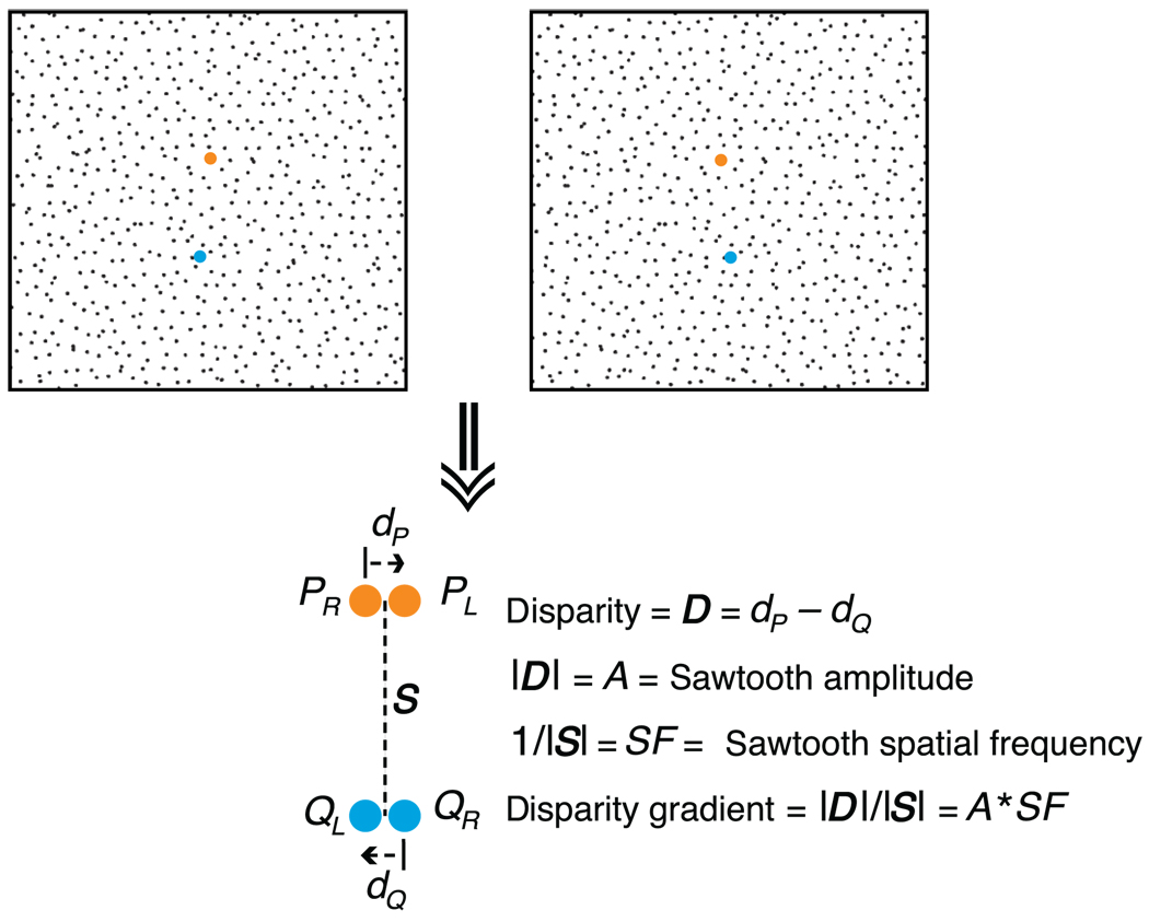
On a surface, the disparity gradient is not clearly defined because the gradient can in principle be measured in any direction. The gradient is, however, largest in the direction in which depth increases most rapidly (i.e., parallel to surface tilt). For this reason, we will define the disparity gradient in the direction of most rapidly increasing depth: i.e., S will be parallel to tilt. The definition of the disparity gradient for a horizontally oriented sawtooth corrugation is schematized in Figure 2.

Figure 2.

Definition of the disparity gradient. The upper part of the figure is a stereogram in which disparity specifies a sawtooth corrugation in depth. The orange and blue points, P and Q, lie on one of the slats of the sawtooth, near the trough and peak of the wave, respectively. They are positioned such that their separation S is aligned with the direction of most rapidly increasing depth. The lower part of the figure shows how the disparity gradient is defined.

The observation that the product of spatial frequency and amplitude must not exceed a critical value is also a manifestation of the disparity-gradient limit. As shown in Figure 2, the disparity gradient for sawtooth slats can be expressed as

$$DG=A*SF,$$ (6)

where A is the amplitude of the sawtooth wave and SF is the spatial frequency. The disparity gradient for the discontinuities between the slats is infinite. While sine waves do not have a constant disparity gradient, the disparity gradient of the steepest part of the waveform will have a similar relationship to the amplitude and spatial frequency. The corrugations in Figure 1 are horizontal (as they were in Tyler, 1973, 1974, 1975) and are defined by horizontal disparity only; thus, S is vertical and D is horizontal.

Why does the disparity-gradient limit exist? There are two general hypotheses. First, the limit might be a manifestation of constraints built into the visual system to help minimize false matches between the two eyes’ images; we will refer to this as the constraint hypothesis. Second, the disparity-gradient limit might be a byproduct of the manner in which binocular correspondence is solved; we will refer to this as the correlation hypothesis.

The constraint hypothesis states that the disparity-gradient limit is a topology constraint. Consider a small frontoparallel surface with a vertical rotation axis (tilt = 0°). As we rotate the surface, the slant increases. At some point, one eye will see the surface “edge on” such that points in the direction of most rapidly increasing depth will be superimposed in one eye’s retinal image and not in the other eye’s image. When this occurs, the disparity gradient is 2 (Trivedi & Lloyd, 1985). If we rotate the surface further, the gradient exceeds 2, and the order of the image points is reversed in the two eyes (specifically, the points occur in opposite orders along an epipolar line in the two eyes’ images). This observation is, however, only correct for surfaces with a tilt of 0° (i.e., when the direction of S and D are both horizontal). Trivedi and Lloyd (1985) argued that the visual system avoids matching elements with different orderings in the two eyes by invoking the disparity-gradient limit. Specifically, matches consistent with a small gradient should be favored over matches with a large one. Invoking a disparity-gradient constraint in solving the correspondence problem is consistent with other constraints that have been proposed such as the uniqueness, ordering, and smoothness constraints (Li & Hu, 1996; Marr & Poggio, 1976; Pollard, Mayhew, & Frisby, 1985; Prazdny, 1985).

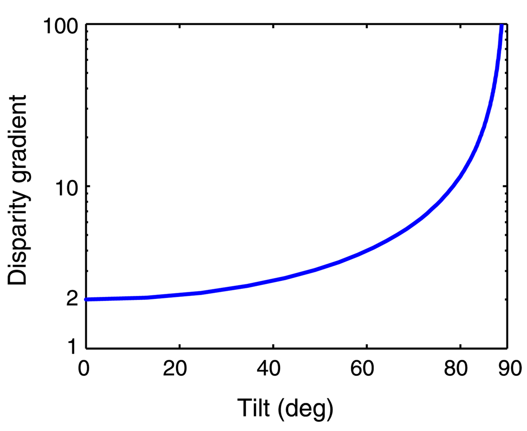
Although Trivedi and Lloyd (1985) showed that ordering is preserved when the disparity gradient is less than 2, they also noted that the converse is not true: all correctly ordered points will not necessarily have a disparity gradient less than 2. To expand this observation, we calculated the disparity gradient at which occlusion occurs in one eye for different surface tilts. Figure 3 shows the results. The critical gradient is indeed 2 at tilt = 0°, but it increases with increasing tilt until it becomes infinite at tilt = 90°. Thus, the value of the disparity gradient at which the order of image points in the two eyes’ images reverses is strongly dependent on surface tilt. If the constraint serves the function of avoiding matches of one element with two in the other eye (uniqueness constraint) or of matching elements in different orders in the two eyes (ordering constraint), one would expect the disparity-gradient limit to increase with increasing surface tilt. The fact that it does not (Burt & Julesz, 1980) suggests that the limit is caused by something else.

Figure 3.

Critical disparity gradient vs. tilt. As the slant of a surface increases, the disparity gradient increases. The critical gradient is the disparity gradient at which one eye’s image is first occluded. The disparity gradient at which this occurs is tilt-dependent. This plot was generated with the eyes in forward gaze; it is unaffected by the eyes’ vergence.

The correlation hypothesis states that the disparity-gradient limit is a byproduct of the fundamental calculation involved in solving the correspondence problem. The normalized cross-correlation (Equation 9) between two images reaches its greatest value of 1 when the two eyes’ images are identical. Spatial variations in disparity cause differences in the two images and thereby cause a decrease in correlation. For this reason, one expects the correlation to decrease as the disparity gradient increases. The decrease in correlation occurs whether the disparity gradient is greatest horizontally (surface with tilt = 0°), vertically (tilt = 90°), or anything in-between. The fact that the disparity-gradient limit is not dependent on tilt is consistent with the correlation hypothesis and not with the constraint hypothesis.

We tested the idea that the disparity-gradient limit is a byproduct of estimating disparity by correlation by examining how the disparity gradient affects human stereopsis, how it affects the performance of a correlation model, and then comparing the two on the same task with the same stimuli.

Human methods

Observers

The observers were the two authors and two other adults; the latter were unaware of the experimental hypotheses. All had normal visual acuity and stereopsis.

Apparatus

Stimuli were displayed on a haploscope consisting of two monochrome CRT displays (58 cm on the diagonal) each seen in a mirror by one eye (Backus, Banks, van Ee, & Crowell, 1999; Hillis & Banks, 2001). The lines of sight from the eyes to the centers of the displays were perpendicular to the display surfaces. The displays were 39 cm from the eyes. Despite the short distance, the visual locations of the elements in our stimuli were specified to within ~30 arcsec. We fixed eye position relative to the displays by using custom bite bars.

Stimuli

The stimuli were random-dot stereograms with a dot density of 10 dots/deg² and an extent of 15° horizontally and vertically. The average luminous intensity of a dot was 1.72 × 10⁻⁶ cd and the size was 0.53 arcmin. The dots were randomly distributed in the half-images. Two methods were used to create disparity. In the first, we shifted the dots horizontally in screen coordinates (which correspond to horizontal in Helmholtz coordinates). This is the most common method for creating stereograms, but such stimuli presented in a haploscope do not have the vertical disparities that are produced by real-world stimuli at finite distances (Held & Banks, 2008). In the second method, we used “back projection” to create the appropriate horizontal and vertical disparities (Backus et al., 1999).

The disparities specified a horizontally oriented sawtooth corrugation (Figure 2). Each slat in the sawtooth had a constant disparity gradient that was proportional to both the spatial frequency and amplitude of the corrugation.

Procedure

Before each trial, a dichoptic nonius fixation target was visible. Observers made sure the nonius lines were aligned before initiating a stimulus presentation, which assured that their vergence eye position was appropriate. With a key press, the observer initiated a 600-ms presentation of the sawtooth stimulus. It was presented in one of two parities: with the slats slanted top-back or top-forward. The observer then indicated which parity had been presented. The absolute phase of the sawtooth was varied randomly from trial to trial, so that the task could not be performed by determining the depth of a single dot. Because the corrugations were horizontal (i.e., tilt = 90°), there were no monocular artifacts; performing the task required perceiving the cyclopean waveform.

We wanted to keep the corrugation waveform fixed for each experimental condition, so we measured parity-discrimination thresholds by adding uninformative noise to the stimulus rather than by manipulating disparity amplitude, which would have changed the disparity gradient of the waveform. The uninformative noise was dots randomly positioned in 3D; the depths of the noise dots were drawn from a uniform random distribution with a fixed range that was greater than the depth range of the corrugation waveform. Coherence is the number of signal dots (those specifying the corrugation) divided by the total number of dots (signal dots plus noise dots). A coherence of 1 means that all dots are signal dots, while a coherence of 0 means that all dots are noise dots. The sum of signal and noise dots was always the same. We varied coherence using the method of constant stimuli in order to determine the threshold value. We fit the psychometric data with a cumulative Gaussian using a maximum-likelihood criterion and used the coherence at 75% correct as the threshold estimate (Wichmann & Hill, 2001).

Our cyclopean discrimination task required that observers perceive at least part of the disparity-defined corrugation. We assume that the two eyes’ images had to be fused to perform this task.

Human results

The first measurements were made with stereograms in which the disparities were created by horizontal shifting. The haploscope arms were rotated such that the vergence distance was 39 cm, which matched the physical distance to the CRTs.

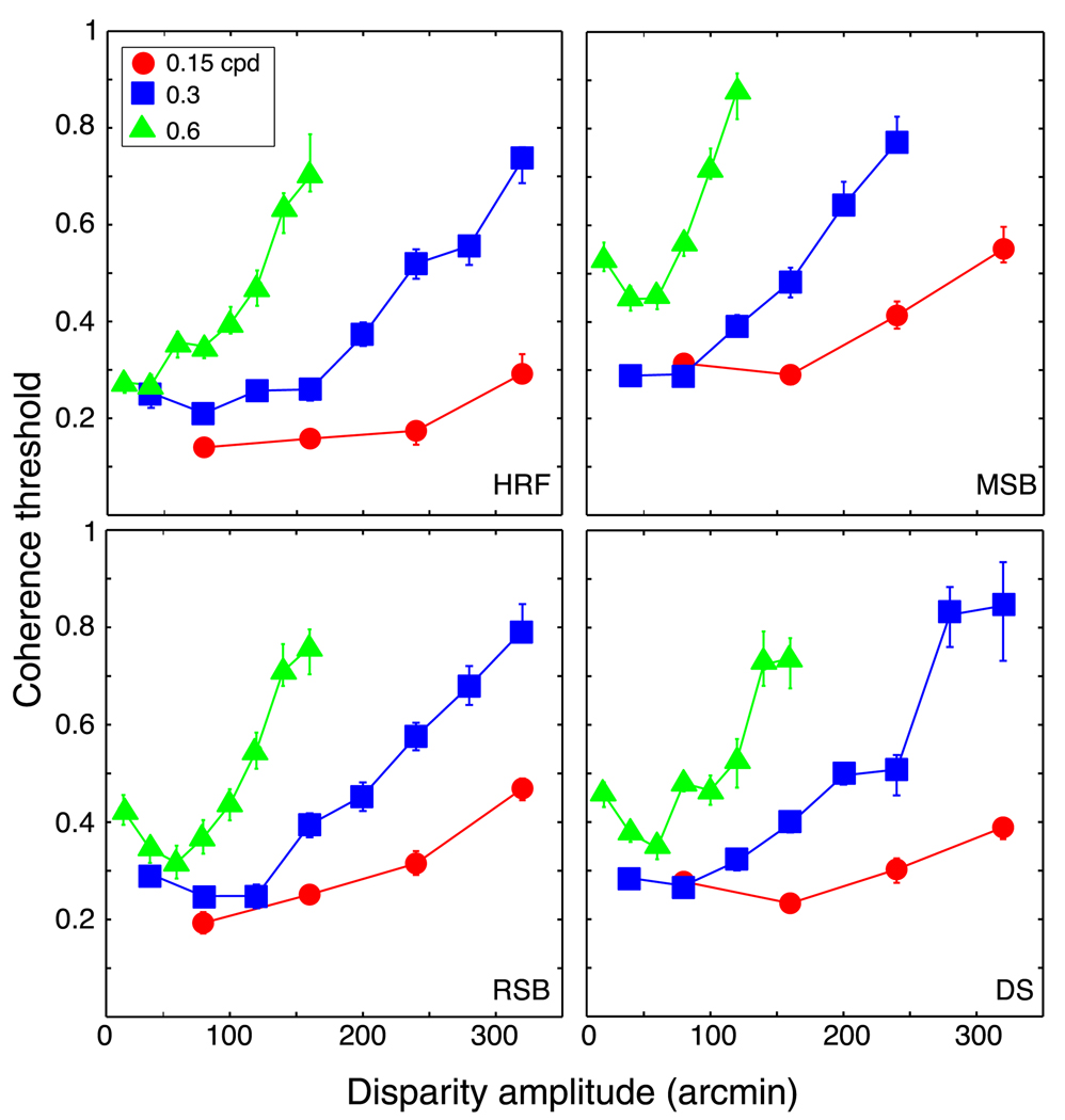
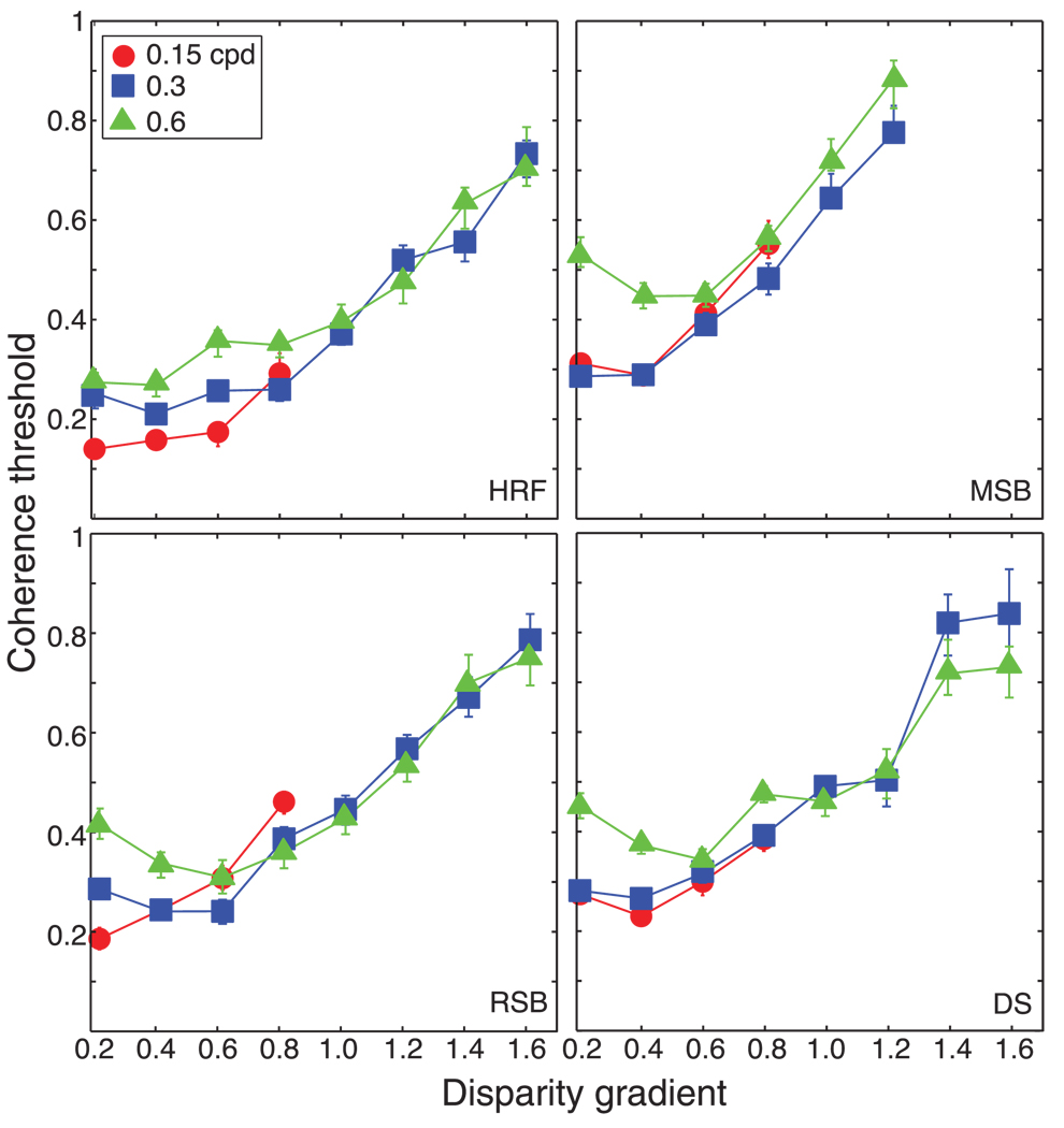
Figures 4 and 5 plot the results. In Figure 4, coherence threshold is plotted as a function of disparity amplitude. The three sets of data points correspond to the thresholds for three different spatial frequencies: 0.15, 0.3, and 0.6 cpd. Coherence threshold generally rose with increasing disparity amplitude, but there was no particular amplitude at which the rise in threshold was the same. Figure 5 plots the same data as a function of disparity gradient. With increasing gradient, threshold rose in similar fashion for all three spatial frequencies. Thus, perception of the cyclopean waveform began to collapse as the disparity gradient reached a value of approximately 1, which is consistent with earlier work (Burt & Julesz, 1980; Tyler, 1973, 1974, 1975; Ziegler et al., 2000). The worsening of performance was not precipitous: observers could still discriminate the cyclopean waveform when the gradient was as high as 1.6. This is consistent with previous work showing that humans can perceive surfaces when the disparity gradient exceeds 1 (McKee & Verghese, 2002).

Figure 4.

Coherence threshold vs. disparity amplitude for human observers. Each panel plots coherence threshold, the proportion of signal dots in the stimulus, as a function of the peak-to-trough disparity amplitude. Different panels show data from different observers. Different symbols represent data for different spatial frequencies of the horizontal sawtooth corrugation: circles, squares, and triangles for 0.15, 0.3, and 0.6 cpd, respectively. Error bars are standard errors of the means calculated by bootstrapping.

Figure 5.

Coherence threshold vs. disparity gradient for human observers. Each panel is replotted from Figure 4. The panels plot coherence threshold, the proportion of signal dots in the stimulus, as a function of the disparity gradient of the slats of the horizontal sawtooth stimulus. Different panels show data from different observers. Different symbols represent data for different spatial frequencies: circles, squares, and triangles for 0.15, 0.3, and 0.6 cpd, respectively. Error bars are standard errors of the means calculated by bootstrapping.

We also measured coherence thresholds for vertically oriented waveforms (tilt = 0°). The task was generally more difficult because vertical corrugations produced severe monocular artifacts (regions in which no dots appeared and regions of high dot density), but we were able to obtain reasonable data from two observers. As with horizontal corrugations, the rise in coherence threshold was determined by the disparity gradient. Thus, the disparity gradient is a key determinant of the ability to perceive cyclopean stimuli whether the variations in depth are vertical (tilt = 90°) or horizontal (tilt = 0°).

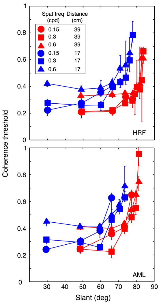
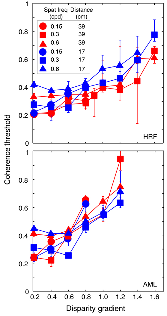
A given disparity gradient specifies different slants at different distances. The first experiment was conducted at one simulated viewing distance, so the relationship between disparity gradient and slant was fixed. It is therefore possible that slant rather than the disparity gradient was the primary limit to performance. To investigate this possibility, we tested two observers at different viewing distances. To vary the simulated distance, we manipulated the vergence stimulus by rotating the haploscope arms to the appropriate values. It was also important to present the appropriate vertical-disparity gradient because this gradient is an effective distance cue (Rogers & Bradshaw, 1993, 1995). We therefore used the back-projection method to create disparities in the stereograms. The vertical-disparity gradient and the horizontal vergence of the back-projected stimuli specified viewing distances of 17 or 39 cm. At 17 cm, a gradient of 1 specifies a slant of 71°; at 39 cm, the same gradient specifies a slant of 80°.

The results are shown in Figures 6 and 7. The data from the two viewing distances nearly superimposed when plotted as a function of disparity gradient (Figure 7) and did not when plotted as a function of slant (Figure 6). Thus, the disparity gradient rather than slant was the primary limit to performance.

Figure 6.

Coherence threshold vs. slant for human observers. Coherence threshold, the proportion of signal dots in the stimulus, is plotted as a function of the slant of the sawtooth slats. Different panels show data from different observers. Different symbol shapes represent data for different spatial frequencies: circles, squares, and triangles for 0.15, 0.3, and 0.6 cpd, respectively. Different colors represent data from the two viewing distances: red and blue for 39 cm and 17 cm, respectively. Error bars are standard errors of the means calculated by bootstrapping.

Figure 7.

Coherence threshold vs. disparity gradient for human observers. Coherence threshold, the proportion of signal dots in the stimulus, is plotted as a function of the disparity gradient of the sawtooth slats. Different panels show data from different observers. Different symbol shapes represent data for different spatial frequencies: circles, squares, and triangles for 0.15, 0.3, and 0.6 cpd, respectively. Different colors represent data from the two viewing distances: red and blue for 39 cm and 17 cm, respectively. Error bars are standard errors of the means calculated by bootstrapping.

The human results show, as others have (Tyler, 1974, 1975; Ziegler et al., 2000), that the disparity gradient is a key determinant of the ability to construct stereoscopic percepts. As the gradient increases, percept construction becomes successively, but not precipitously, more problematic. The constraints imposed by high disparity gradients do not depend on stimulus tilt. We next examined the cause of the degradation in performance with increasing disparity gradient.

Modeling methods

If the constraints imposed by large disparity gradients are a byproduct of estimating disparity via correlation, we should see similar behavior in humans and a local cross-correlator like the one described by Banks et al. (2004). As noted earlier, such a correlation algorithm has the same fundamental properties as the disparity-energy calculation that characterizes binocular neurons in visual cortex (Anzai, Ohzawa, & Freeman, 1999; Ohzawa et al., 1990).

Stimuli and task

We presented the same stimuli and task to the model that were presented to human observers. The stimuli were again random-dot stereograms specifying sawtooth corrugations and the task was again to determine the parity of the sawtooth.

The stereo half-images were blurred according to the optics of the human eye. Specifically, we convolved the half-images with the point-spread function of the well-focused eye with a 3-mm pupil (h(x, y)):

$$h(x,y)=a*h_1(x,y)+(1-a)*h_2(x,y),$$ (7)

where

$$h_i(x,y)={\left[\sqrt{2\pi }{s}_i\right]}^{-2}{e}^{-0.5(x^2+y^2)/s_i^2}$$ (8)

and a = 0.583, s₁ = 0.443 arcmin, and s₂ = 2.04 arcmin (Geisler & Davila, 1985). The resulting images were scaled such that the spacing between rows and columns was 0.6 arcmin, corresponding roughly to the spacing between foveal cones (Geisler & Davila, 1985). These values were chosen to best approximate the analogous viewing situation for the human observers.

Cross-correlator

The half-images were then sent to the binocular cross-correlator, which computed the correlation between samples of the left and right half-images:

$$c({\delta }_x)=\frac{{\displaystyle \sum _{(x,y)\in W_L}[(L(x,y)-{\mu }_L)(R(x-{\delta }_x,y)-{\mu }_R)]}}{\sqrt{{\displaystyle \sum _{(x,y)\in W_L}{(L(x,y)-{\mu }_L)}^2}}\sqrt{{\displaystyle \sum _{(x,y)\in W_R}{(R(x-{\delta }_x,y)-{\mu }_R)}^2}}},$$ (9)

where L(x, y) and R(x, y) are the image intensities in the left and right half-images, W_L and W_R are the windows applied to the half-images, µ_L and µ_R are the mean intensities within the two windows, and δ_x is the displacement of W_R relative to W_L (where the displacement is disparity). The normalization by mean intensity assures that the correlation is always between −1 and 1; the correlation for identical images is 1. Without the normalization, the resultant would depend on the contrast and average intensity of the half-images. W_L and W_R were identical two-dimensional Gaussian weighting functions:

$$W_L=W_R=e^{-\left(\frac{x^2}{2{\sigma }_x^2}+\frac{y^2}{2{\sigma }_y^2}\right)}.$$ (10)

We used isotropic functions, so σ_x and σ_y had the same values (for an example of the use of anisotropic functions, see Kanade & Okutomi, 1994). These weighting functions were used to select patches of the left and right half-images, which were then cross-correlated. Throughout the manuscript, we refer to the size of these weighting functions as “window size”; the window size we report is the diameter of the part of the Gaussian containing ±1σ. The actual windows used in the simulations extended to ±3σ until they were truncated. Our weighting functions mimic the envelopes associated with cortical receptive fields, but not the even- and odd-symmetric weighting functions of the disparity-energy model (Ohzawa et al., 1990).

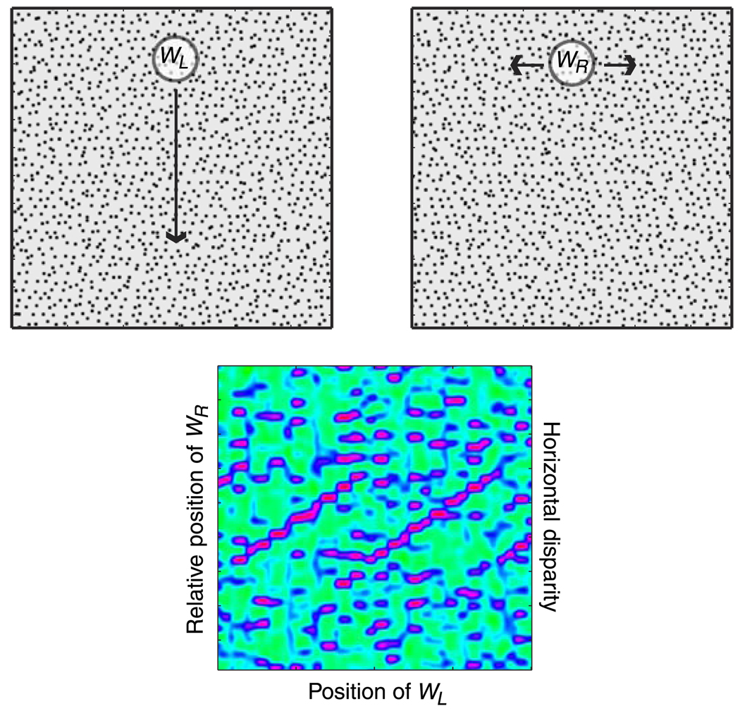
To estimate disparity across the stimulus, we shifted W_L along a vertical line perpendicular to the sawtooth corrugations in the middle of the left eye’s half-image. For each position of W_L, we then computed the correlation for different horizontal positions of W_R relative to W_L (Equation 9; horizontal defined in Helmholtz coordinates). The restriction of shifting W_L along one vertical line greatly reduced computation time but did not affect the main results.

The lower part of Figure 8 provides an example of the output of the cross-correlator. The abscissa represents the position of W_L along the vertical search line and the ordinate represents the horizontal position of W_R relative to W_L; thus, the ordinate is the horizontal disparity. Red corresponds to high correlations, green to correlations near 0, and blue to negative correlations.

Figure 8.

Local cross-correlation model for disparity estimation. The upper two panels are the half-images presented to the model. The reader can see the sawtooth corrugation by divergent or cross fusing. A Gaussian correlation window W_L is placed in the left eye’s half-image. That window was moved along a vertical line as indicated by the arrow. For each position of W_L, an identical Gaussian window W_R was placed in the right eye’s image, and the cross-correlation (Equation 9) was computed between the two windowed images. Throughout the manuscript, we refer to the size of W_L and W_R as the “window size.” By this we mean two standard deviations of the Gaussian. The lower panel shows an example of the output of the cross-correlator. The abscissa is the position of W_L along the vertical line in the left eye’s image, and the ordinate is the relative horizontal position of W_R; this corresponds to the horizontal disparity. Correlation is represented by color, red for correlations approaching 1, green for correlations near 0, and blue for correlations between −1 and 0. In this example, the sawtooth is revealed by ridges of high correlation.

Decision rule

To compare model and human behaviors for the same task, we needed a decision rule for the model. It would have been best to use an ideal decision rule because such a rule is information preserving and is therefore best at revealing constraints imposed by earlier processing stages (Watson, 1985). However, to construct an ideal rule, we would need to know the means and standard deviations for each pixel in the correlation image for all the relevant parameters. The required computation was too complex and time consuming, so we chose a simpler rule: template matching (Watson, Barlow, & Robson, 1983). We first constructed templates of the post-optics stimuli in disparity-estimation space. Specifically, we constructed a bank of templates with the same dimensions as the cross-correlator output. Each template in this bank had the same spatial frequency as the corrugation waveform. All relevant amplitudes were included as were the two parities. To minimize computation time, phase was varied in steps of 10° (the phase of the stimulus was also limited to 10° steps). We next found the similarity of each template to the output of the cross-correlator by using an abbreviated form of cross-correlation: each template was multiplied element by element by the cross-correlator output and the result was summed across both dimensions. The model then picked the stimulus whose template had the highest correlation with the cross-correlator output. The model therefore knew the spatial frequency of the stimulus but was uncertain about everything else. By recording the model’s responses, we were able to construct psychometric functions like the ones generated in the human experiments. These functions were fit by cumulative Gaussians using a maximum-likelihood criterion; the threshold estimates were the means of the best-fitting functions (Wichmann & Hill, 2001).

Modeling results

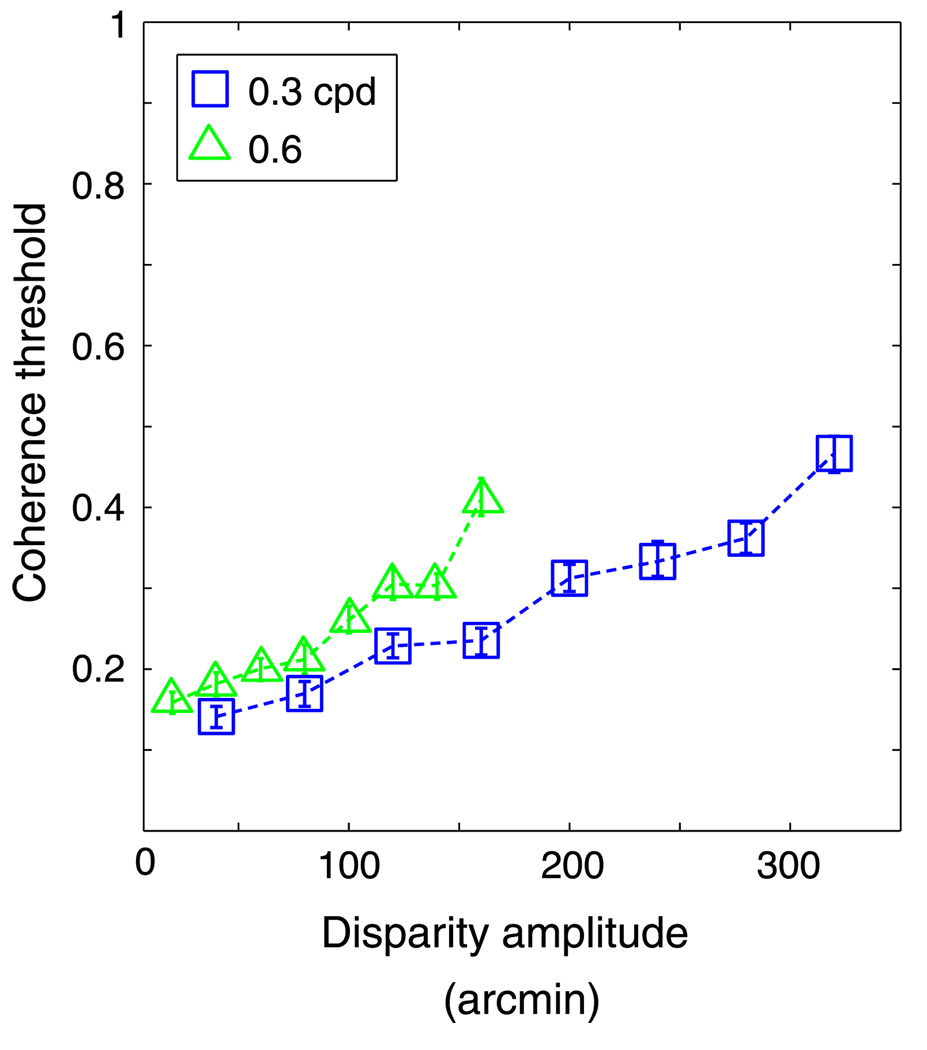
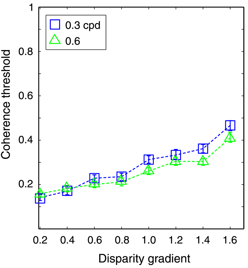
The results are shown in Figures 9 and 10. In Figure 9, the model’s coherence threshold is plotted against disparity amplitude. Threshold rose with increasing amplitude, but at different rates depending on the spatial frequency of the horizontal corrugation stimulus. In Figure 10, the same data are plotted as a function of disparity gradient. Now the curves superimpose, so the disparity gradient, not the disparity amplitude, was the primary constraint for the local cross-correlator.

Figure 9.

Coherence threshold vs. disparity amplitude for the cross-correlation model. Coherence threshold, the proportion of signal dots in the stimulus, is plotted as a function of the disparity amplitude of the horizontal sawtooth stimulus. The size of the correlation window used in this simulation was 18 arcmin (recall that refers to ±1 standard deviation of the Gaussian window). Different symbols represent different spatial frequencies: squares and triangles for 0.3 and 0.6 cpd, respectively. Error bars are standard errors of the means calculated by bootstrapping.

Figure 10.

Coherence threshold vs. disparity gradient for the cross-correlation model. Coherence threshold is plotted as a function of the disparity gradient of the sawtooth slats. The size of the correlation window was 18 arcmin. Different symbols represent different spatial frequencies: squares and triangles for 0.3 and 0.6 cpd, respectively. Error bars are standard errors of the means calculated by bootstrapping.

We also conducted simulations with vertically oriented sawtooth corrugations and observed quite similar behavior (not shown).

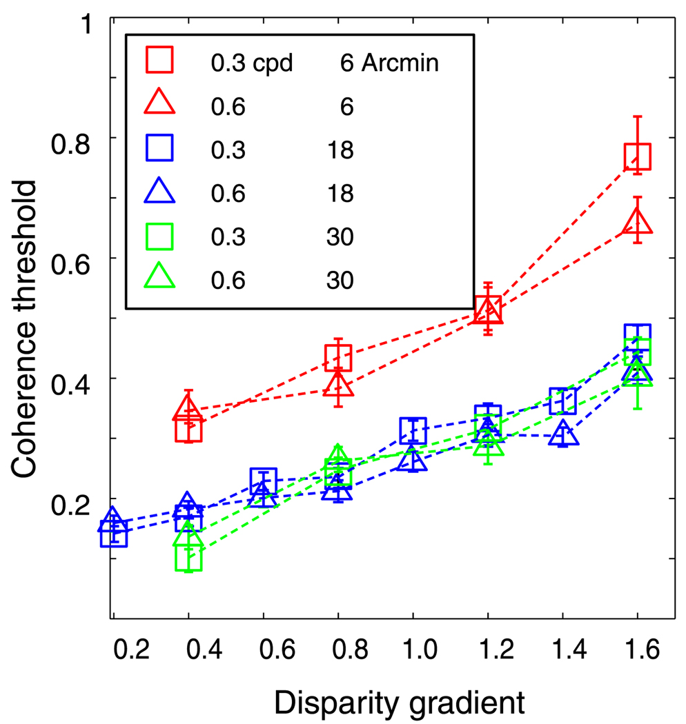
The size of the window used to correlate the two eyes’ images is an important aspect of disparity estimation (Banks et al., 2004; Harris et al., 1997; Kanade & Okutomi, 1994). Larger windows contain more variation in luminance and thus generally allow better discrimination between correct and false matches. However, when disparity varies at a finer scale than the window, the ability to estimate the variation is reduced. To investigate the influence of window size on disparity estimation, we ran the local cross-correlator with window sizes of 6, 18, and 30 arcmin. Figure 11 shows the results. For every window size, threshold grew systematically with an increase in disparity gradient, and the growth was the same for different spatial frequencies. Thus, the fall-off in performance with increasing disparity gradient is similar regardless of the size of the correlation window. Overall performance was somewhat reduced with the smallest window of 6 arcmin because the dot density of 10 dot/deg² was too low to provide sufficient luminance variation over that small a region. We conclude that disparity estimation via correlation suffers from a disparity-gradient limit, and that the limit cannot be avoided by choosing smaller window sizes.

Figure 11.

Coherence threshold vs. disparity gradient for the cross-correlation model with different window sizes. Different colors represent thresholds obtained for different sizes of the correlation window: red for 6 arcmin, blue for 18 arcmin, and green for 30 arcmin. Different symbol types represent thresholds for different spatial frequencies: squares and triangles for 0.3 and 0.6 cpd, respectively. Error bars are standard errors of the means calculated by bootstrapping.

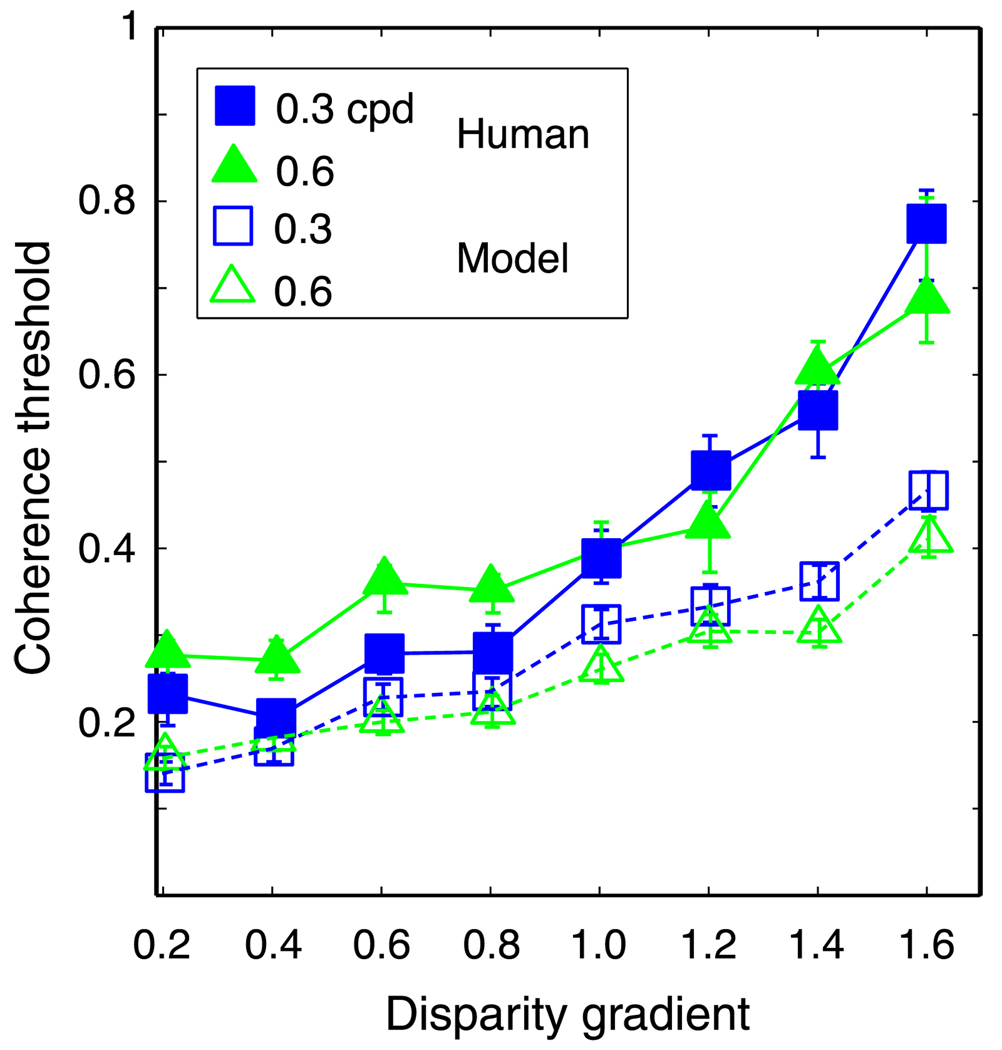
We next compared the performance of the local cross-correlator model with human performance. Figure 12 plots coherence thresholds for the model and a representative human observer for the same stimulus and task. In both cases, the rise in threshold was determined by the disparity gradient, not the disparity amplitude. Thus, the human visual system is constrained in much the same way as a local cross-correlator when it is presented two images that differ greatly.

Figure 12.

Comparison of model and human performances. Coherence thresholds are plotted as a function of disparity gradient for the local cross-correlator and a representative human observer (HRF). Filled symbols are human data and unfilled symbols are model data. The size of the correlation window used in this simulation was 18 arcmin. Different symbols represent different spatial frequencies: squares and triangles for 0.3 and 0.6 cpd, respectively. Error bars are standard errors of the means calculated by bootstrapping.

There was one systematic difference between human and model behaviors: The rise in threshold as a function of disparity gradient was steeper in humans. This difference is probably caused by differences in the way large absolute disparities are treated by humans and the model. In humans, disparity-discrimination thresholds increase with the value of absolute disparity because disparity estimation is not as precise off the horopter as it is near the horopter (Blakemore, 1970; Ogle, 1953). Furthermore, the detection of correlation in dichoptic stimuli worsens systematically with increases in absolute disparity (Stevenson, Cormack, Schor, & Tyler, 1992). As the disparity gradient increased in our experiment, more of the stimulus fell farther from the horopter, which would have made it more difficult for humans to perceive the signal corrugation. Our model had no provision for penalizing solutions involving large disparities, so it did not suffer in the same way as humans when parts of the stimulus created large absolute disparities.

In summary, the disparity gradient of a stimulus is a critical determinant of humans’ ability to construct stereoscopic percepts. Its influence seems to be unaffected by the orientation or tilt of the depth variations. These same properties are exhibited by a local cross-correlation model. Thus, the disparity-gradient limit appears to be a byproduct of using this method to estimate disparities.

Stereoresolution

Although humans can detect very small disparities, stereoresolution—the finest spatial variation in disparity that can be reliably perceived—is relatively poor (Bradshaw & Rogers, 1999; Tyler, 1973, 1974, 1975). The highest detectable spatial frequency for disparity-defined corrugations is only 2–3 cpd (Figure 1); in contrast, the highest detectable frequency for luminance-defined waveforms is about 50 cpd (Campbell & Robson, 1968). Banks et al. (2004) proposed that relatively coarse stereoresolution is a byproduct of estimating disparity by correlating the two eyes’ images. To further investigate this possibility, we compared the performance of humans and the local cross-correlator in the same stereoresolution task.

Human methods

The human data are from Banks et al. (2004); here we describe the most important aspects of the methods; for details, refer to the original paper.

Stimuli

The stimuli were random-dot stereograms specifying sinusoidal corrugations in depth. The orientations of the corrugations were ±20° from horizontal. There were two viewing distances: 39 and 154 cm. At the shorter viewing distance, the stimuli were viewed using the haploscope described in the disparity-gradient experiment. At the longer distance, the CRTs were detached from the haploscope arms and the stimuli were free-fused. The stimuli subtended 35.5 × 35.5° and 9.3 × 9.3° at the short and long distances, respectively. The apparent positions of the dots were accurate to better than 30 and 8 arcsec at the two distances. By using nearly horizontal corrugations, we minimized monocular artifacts (signal-dependent changes in dot density in the monocular half-images). We varied dot density in the half-images from 0.15 to 145 dots/deg². The disparity amplitude was 4.8 and 16 arcmin.

Procedure

Stimuli were presented for 600 ms at the shorter viewing distance and 1500 ms at the longer one. After each presentation, observers indicated which of the two corrugation orientations had been presented. The spatial frequency of the corrugation was varied by an adaptive staircase procedure to find the just-discriminable value.

Human results

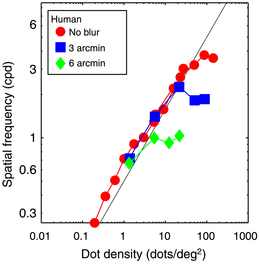
Figure 13 plots human stereoresolution as a function of dot density. The three curves represent the data when different amounts of spatial blur were applied to the half-images.

Figure 13.

Stereoresolution vs. dot density for human observers. The just-discriminable spatial frequency of the sinusoidal corrugation waveform is plotted as a function of dot density. The data are the averages for the two tested observers, JMA and MSB. Circles, squares, and diamonds represent the results, respectively, for stimuli that were not blurred, stimuli blurred by a Gaussian kernel whose standard deviation was 3 arcmin, and stimuli blurred by a Gaussian whose standard deviation was 6 arcmin. The black diagonal line represents the Nyquist frequency.

The red circles represent the data when no blur was applied. For this condition, resolution increased systematically with increasing density until reaching a plateau at 3–4 cpd. The initial rise in resolution is understandable from sampling considerations. In random-dot stereograms, the discrete dot sampling in the half-images limits the highest frequency one can reconstruct to the Nyquist sampling frequency:

$$f_N=\frac{1}{2}\sqrt{\frac{N}{A}},$$ (11)

where N is the number of dots and A is the stimulus area. The diagonal line in Figure 13 is f_N for the various dot densities. Human stereoresolution followed this sampling limit up to a density of ~30 dots/deg², so the highest resolvable spatial frequency was determined by dot sampling in the half-images at low to medium densities. At higher densities, it was restricted by something else. Banks et al. (2004) showed that the restriction was not the disparity-gradient limit; they showed this by reducing disparity and thereby reducing the disparity gradient, and observing that the asymptotic spatial frequency was unaffected.

A logical candidate for the cause of the asymptote is low-pass spatial filtering at the front end of the visual system because such filtering limits performance in many resolution tasks including luminance contrast sensitivity at high spatial frequency (Banks, Geisler, & Bennett, 1987; Banks, Sekuler, & Anderson, 1991; MacLeod, Williams, & Makous, 1992) and various types of visual acuity (Levi & Klein, 1985). Banks et al. (2004) examined the contribution of low-pass spatial filtering to stereoresolution by blurring the stimulus. Such filtering reduces fine-scale luminance variation in the half-images. The three sets of curves in Figure 13 represent the data when different amounts of blur were applied. Stereoresolution always followed the Nyquist frequency at low densities and always asymptoted at higher densities. The asymptotic resolution was ~4 cpd when the standard deviation of the stimulus blur was 0, ~2 cpd when the standard deviation was 3 arcmin, and ~1 cpd when it was 6 arcmin. Thus, stereoresolution in humans is limited by the sampling properties of the stimulus at low dot densities and seems to be limited by the luminance spatial-frequency content of the half-images at high densities.

We examined these determinants further by comparing human behavior to the behavior of the cross-correlator. We did so for the same stimuli and task in order to determine whether the relatively coarse stereoresolution of the human visual system is a byproduct of using correlation to estimate disparity.

Modeling methods

The stimuli and task were nearly identical to those in Banks et al. (2004). Sine wave corrugations were presented with orientations that were ±10° from horizontal. The model judged on each presentation which orientation had been presented. The spatial frequency of the corrugations was varied to find the highest value for which orientation discrimination was 75% correct. We varied dot density from 0.6 to 300 dots/deg². Peak-to-trough disparity amplitude was fixed at 10 arcmin, a value midway between the values of 4.8 and 16 arcmin used in Banks et al. (2004). For some modeling runs, we blurred the half-images with isotopic Gaussians before presenting them to the rest of the model.

The properties of the model were identical to those in the analysis of the disparity-gradient limit with the following exceptions.

1. Window size was varied over a different range. As before, portions of the half-images were selected with isotropic Gaussian windows, but window sizes were now varied from 1.5 to 60 arcmin.

2. The window in the left eye was translated in two directions, +10° and −10° from horizontal, corresponding to directions parallel to the two stimulus orientations.

3. The decision templates were also oriented +10° and −10° from horizontal.

4. The templates included both the tested spatial frequencies and half those values.

When the stimulus frequency exceeded the Nyquist frequency, aliases were created. Because of this, a lower frequency template fit the stimulus as well as a template at the stimulus frequency. By including alias templates, we did not unfairly bias the model toward picking the correct template. As in the human experiments, the model did not know the spatial frequency of the stimulus but did know the amplitude.

Modeling results

Banks et al. (2004) argued that there are two primary limiting factors in estimating disparity via correlation: the rate at which disparity changes spatially relative to the correlation window and the amount of luminance variation within the correlation window. With respect to the first factor, the cross-correlator should fail to detect disparity variation when the variation occurs at too fine a spatial scale relative to the size of the window because the correlation signal is adversely affected and because the now noisier disparity estimate at each position will smear rather than follow the spatial variation. As a consequence, the highest correlation frequency the cross-correlator can resolve should level off at a value that is inversely proportional to window size: f_A ∝ 1/w, where f_A is the asymptotic spatial frequency and w is the window size. The model should be able to detect disparity variation at a finer scale simply by using smaller windows. However, for each window size there should also be a dot density below which estimation fails because the number of dots falling within the correlation window becomes on average too small, and correlation rises for false matches leading to failures in disparity estimation. From this argument, the limiting dot density would be inversely proportional to window area: d ∝ 1/w². Thus, for each combination of corrugation frequency and dot density, there should be an optimal size for the correlation window, a size constrained by the two limiting factors.

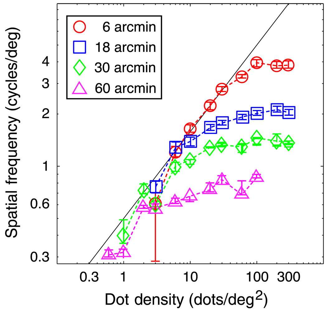
We investigated whether the stereoresolution of the cross-correlation model follows these expectations. Figure 14 shows the model’s stereoresolution as a function of dot density; different symbols represent resolution for correlation windows of different sizes. In each case, the model’s stereoresolution followed the Nyquist frequency up to a particular dot density and then leveled off.

Figure 14.

Stereoresolution vs. dot density for the local cross-correlation model. The just-discriminable spatial frequency of the sinusoidal corrugation waveform is plotted as a function of dot density. Different symbol types represent the results for different sizes of the correlation window: circles for a standard deviation of the Gaussian window of 3 arcmin, squares for a standard deviation of 9 arcmin, diamonds for a standard deviation of 15 arcmin, and triangles for a standard deviation of 30 arcmin. The legend shows ±1 standard deviation of the correlation window. Error bars are standard errors of the means calculated by bootstrapping. The diagonal line represents the Nyquist frequency.

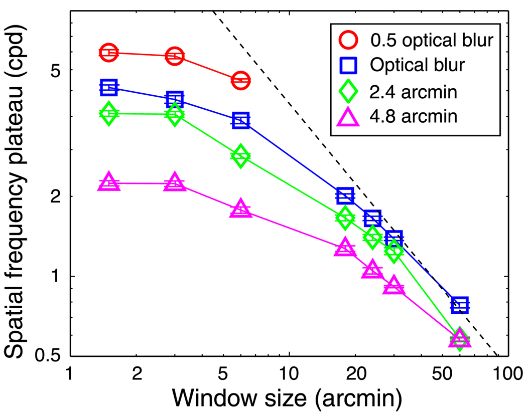
We next investigated the asymptotes where performance fell short of the Nyquist frequency. To examine the possibility that low-pass spatial filtering at the front end of the visual system limits stereoresolution, we manipulated the blur of the images delivered to the cross-correlation stage (Equation 8) and re-measured the model’s stereoresolution. We manipulated blur by varying the blur of the stimulus and the optical point-spread function of the pre-correlation stages. Figure 15 plots the asymptotic spatial frequency against window size for different amounts of blur. The squares, diamonds, and triangles represent the results when the optical point-spread function was the standard for the well-focused eye (Geisler & Davila, 1985) and before entering the eyes the stereo half-images were convolved with isotropic Gaussians with standard deviations of 0, 2.4, and 4.8 arcmin, respectively. The circles represent the results when the spread of the optical function was half the standard value and no blur was applied to the stimulus before entering the eyes. For large windows, the data are well fit by f_A = 45/w (diagonal line; f_A in cpd and w in arcmin). (The absolute values of the spatial frequency plateaus can depend on other stimulus parameters, such as disparity amplitude, but a description of the effects of those parameters is beyond the scope of this paper.) For smaller window sizes, however, the asymptotic frequency leveled off at values lower than predicted. Those asymptotic frequencies depended strongly on blur magnitude: lower asymptotes for greater blur. Thus, there are two things that limit the highest discriminable corrugation frequency: the size of the correlation window (summarized by f_A = 45/w), and the blur associated with the images sent to the cross-correlator (with greater blur, the luminance variation is insufficient to yield robust correlations between the two eyes’ images).

Figure 15.

Spatial frequency asymptote vs. window size. Different symbols represent different amounts of blur: Circles for half the normal optical blur, squares for regular optical blur, diamonds for stimuli blurred by a 2.4-arcmin Gaussian kernel (plus normal optical blur), and triangles for stimuli blurred by a 4.8-arcmin Gaussian kernel (plus normal optical blur). The dashed black line represents the equation f_A = 45/w.

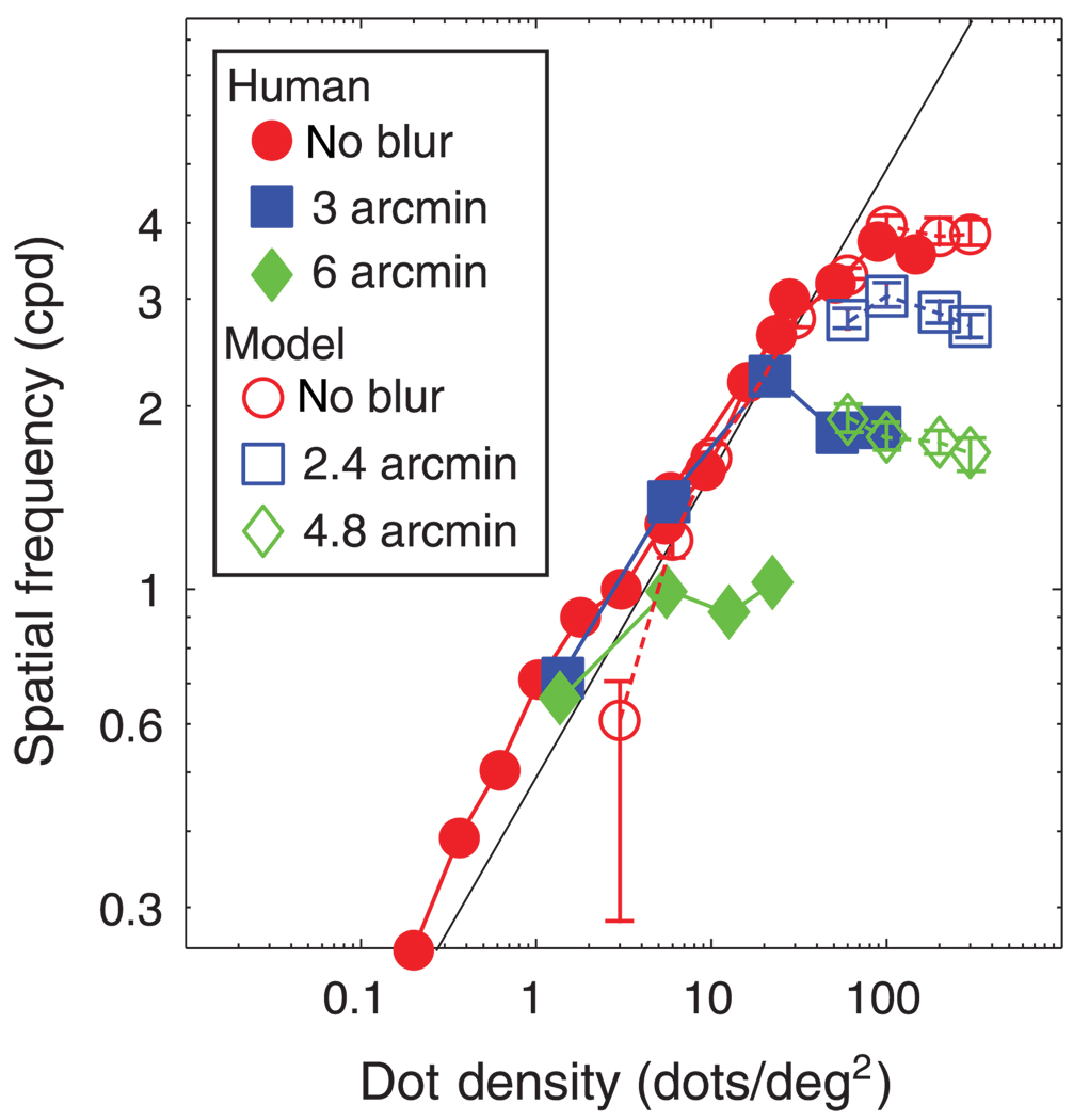
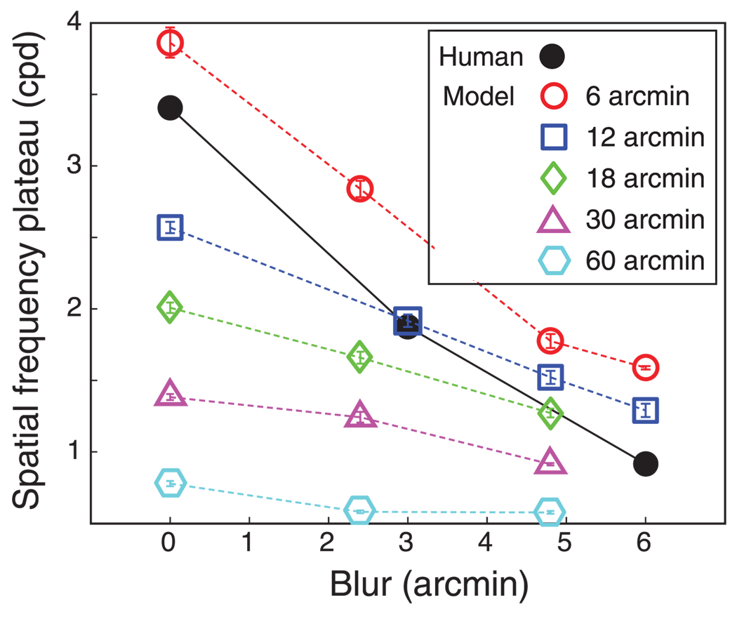
The most important issue: Is the model’s stereoresolution similar to humans? Figure 16 plots model and human stereoresolutions for similar conditions. The similarity is striking. In both cases, resolution grew with increasing dot density in a fashion limited by the Nyquist frequency until it leveled off at a particular spatial frequency. The asymptotic spatial frequency of the model and humans was inversely related to the magnitude of spatial blur. To examine whether the effect of blur was similar in machine and man, we plotted in Figure 17 the humans’ and model’s asymptotic frequencies as a function of blur magnitude along with the model’s asymptotic frequencies. We could manipulate the size of the model’s correlation window, but we obviously could not directly manipulate the size of the mechanism humans use. It is significant to note, however, that the model’s stereoresolution is most similar to human resolution when the model’s window size was set to 6 arcmin: the slopes of the two lines are nearly the same.

Figure 16.

Stereoresolution vs. dot density for the local cross-correlation model and human observers. Filled symbols and solid lines represent the human data and unfilled symbols and dashed lines represent model data. Different symbol types represent different blur magnitudes as indicated by the legend. The values in the legend are the standard deviations of the Gaussian blur kernel applied to the stimuli. Error bars are standard errors of the means calculated by bootstrapping. The diagonal line represents the Nyquist frequency.

Figure 17.

Spatial frequency asymptote vs. blur for model and human results. Filled symbols and solid lines represent the human data and unfilled symbols and dashed lines represent model data. Different symbols represent different window sizes: circles, squares, diamonds, triangles, and hexagons for 6, 12, 18, 30, and 60 arcmin, respectively. Blur values are the standard deviation of the Gaussian kernel applied to the stimulus. Error bars are standard errors of the means calculated by bootstrapping.

We also found, as expected, that for each window size the dot density had to be greater than ~150/w² (where dot density is in dots/deg² and w is in arcmin) for the model to estimate disparity reliably. Thus, we were able to confirm that there is indeed an optimal window size for each combination of corrugation frequency and element density (Banks et al., 2004; Kanade & Okutomi, 1994).

Discussion

Disparity estimation by local cross-correlation has been a useful tool in computer vision (Clerc & Mallat, 2002; Kanade & Okutomi, 1994) and physiology (Cumming & DeAngelis, 2001; Ohzawa, 1998; Ohzawa et al., 1990). Now we see that it can explain some important limitations in human vision as well: namely, our inability to perceive large disparity gradients and our comparatively low stereoresolution. The primary difficulty in using local cross-correlation to estimate disparities is choosing an appropriate size for the image patches sampled in each eye (Banks et al., 2004; Kanade & Okutomi, 1994). Using patches that are too large leads to lower stereoresolution, while patches that are too small may not contain enough luminance variation to enable a reliable disparity estimate (Figure 14). This trade-off between the consequences of using too large or too small a correlation window is fundamental to understanding the disparity-gradient limit and stereoresolution.

What determines the size of the smallest correlation window?

As shown in Figure 14, smaller windows generally permit higher stereoresolution, but windows smaller than ~6 arcmin do not yield significant improvements (Figure 15): with optical blur equivalent to the well-focused eye (Geisler & Davila, 1985), the finest discernible corrugation frequency levels off at ~4 cpd no matter what the window size is. Why does decreasing the window size below ~6 arcmin no longer improve the model’s stereoresolution? The answer becomes clear by considering the blur of the inputs to the cross-correlation stage. When we added blur to the stimulus, thereby increasing the input blur, stereoresolution worsened. When we subtracted blur from the inputs by improving the eyes’ optics beyond normal, stereoresolution improved, particularly for window sizes smaller than 6 arcmin. The unfilled symbols in Figure 17 represent the model’s asymptotic corrugation frequency as a function of stimulus blur for different window sizes; the filled symbols represent human asymptotic frequencies as a function of stimulus blur. Interestingly, model and human behaviors are most similar when the model’s window size was 6 arcmin; the model’s threshold frequencies were slightly higher (perhaps because it uses a more efficient decision rule than humans), but the effect of blur was the same when window diameter was 6 arcmin. This suggests that the smallest mechanism in humans has a diameter of roughly 3–6 arcmin, which is the smallest useful size given the optics of the human eye.

Harris et al. (1997) also attempted to determine the smallest spatial mechanism used in disparity estimation. They measured the ability to judge whether a central dot was farther or nearer than surrounding dots as a function of the disparity of the central dot and its separation from the surrounding dots. They compared human performance in that task with that of a binocular-matching algorithm that correlated the two eyes’ images. Human and model performances were most similar when the width of the model’s square correlation window was 4–6 arcmin. In our analysis, we concluded that the smallest mechanism used by human observers has a diameter of 3–6 arcmin (twice the standard deviation of the Gaussian envelope). Thus, despite differences in the psychophysical tasks, we and Harris et al. (1997) both conclude that the smallest useful mechanism in disparity estimation has a diameter of 3–6 arcmin.

How constraining is the disparity-gradient limit in everyday vision?

As Burt and Julesz (1980) showed, the disparity-gradient limit constrains the fusibility of multiple objects. Because of this limit, a visible point creates zones in front of and behind itself within which a second point cannot be fused. The limit is independent of the direction in which the gradient is measured (i.e., independent of the direction of S in Equation 3), so the forbidden zones are cones with their apices at each visible point.

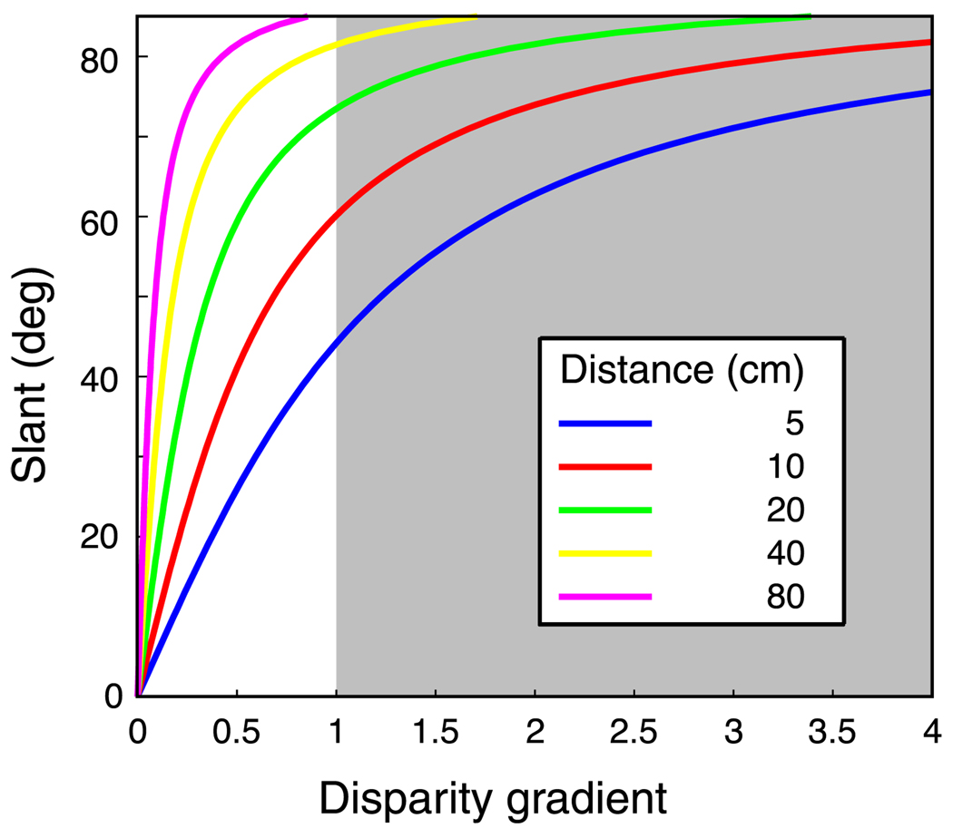
How constraining is the disparity-gradient limit for everyday vision? To examine this question, we calculated the slants that correspond to different disparity gradients for a variety of distances; the geometric relationship between slant and disparity gradient is tilt independent, so the calculations are valid for horizontal-disparity gradients in any direction. Figure 18 shows the results. For a typical reading distance of 40 cm, a disparity-gradient limit of 1 means that opaque surfaces with slants greater than ±80° cannot be readily perceived stereoscopically. Moreover, slants of 80° or more are relatively unlikely to stimulate a given part of the retina. If slants (S) are uniformly distributed in the world, the distribution of slants that stimulate a region in the retina is proportional to cos(S) defined from −90° to +90° (Arnold & Binford, 1980; Hillis, Watt, Landy, & Banks, 2004). As a consequence, it is quite uncommon for a given part of the retina to be stimulated by slants sufficiently large to exceed the disparity-gradient limit at distances of 40 cm and beyond. We conclude that the gradient limit is generally not problematic for everyday viewing of opaque surfaces. Gradients exceeding the disparity-gradient limit are much more likely when viewing transparent surfaces (Akerstrom & Todd, 1988).

Figure 18.

Slant as a function of the disparity gradient for different viewing distances. To generate this plot, we created small opaque surface patches that were rotated about a horizontal axis (tilt = 90°). The disparity gradient was defined as the horizontal disparity divided by the separation in the direction of most rapidly increasing depth. The shaded region represents the gradients that exceed the nominal disparity-gradient limit of 1 (Burt & Julesz, 1980). This plot would be quite similar for other surface tilts.

The disparity-gradient limit and disparity direction

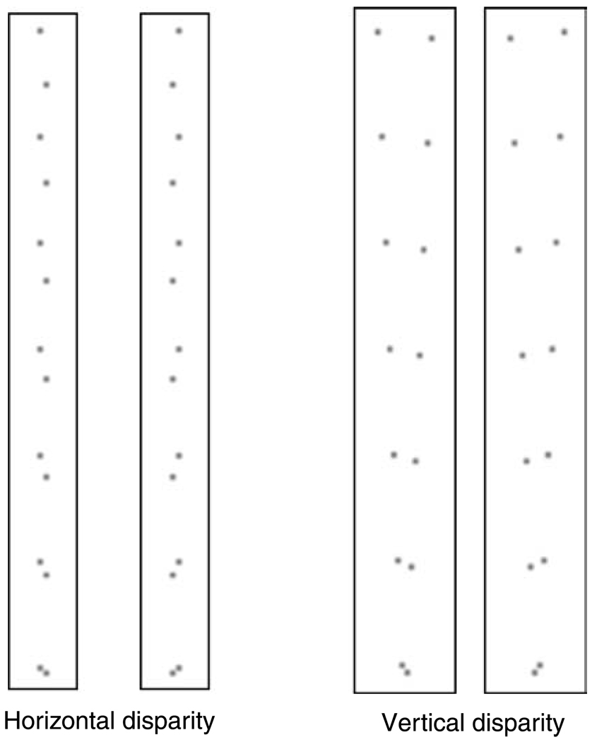
In Equations 2–5, we defined the disparity gradient between two points on a surface as |D|/|S|, where D is the vector representing the binocular disparity between the points and S is the vector representing the separation between them. As far as we know, all previous investigations of the disparity-gradient limit have only considered horizontal disparities. We have argued here that the disparity-gradient limit is caused by the decrease in local cross-correlation that occurs when the two eyes’ images become too different, as happens with large disparity gradients. From this point of view, it should make little difference whether the images differed horizontally or vertically. We wondered, therefore, whether a similar disparity-gradient limit applies for vertical disparity. Figure 19 demonstrates that such a limit does exist for vertical disparity and that the critical value is about the same as it is for horizontal disparity.

Figure 19.

Demonstration of disparity-gradient limits for horizontal and vertical disparities. The left panels demonstrate the disparity-gradient limit when the disparity D between two dots is horizontal and the separation S is vertical. Thus, the dot pairs contain a vertical gradient of horizontal disparity. D is constant for all of the dot pairs, but the magnitude of S decreases from top to bottom, and therefore the disparity gradient |D|/|S| increases from top to bottom. Cross fuse or divergently fuse the half-images and observe the cyclopean image. Most viewers find that fusion breaks and diplopia ensues for the fifth or sixth dot pair from the top, where the disparity gradient is ~1. The right panels demonstrate the disparity-gradient limit when D is vertical and S is horizontal (the magnitudes of D and S are unchanged). Thus, the dot pairs contain a horizontal gradient of vertical disparity. Again D is constant for all dot pairs and |S| decreases from top to bottom, so the disparity gradient increases from top to bottom. Cross fuse or divergently fuse the half-images. Most viewers again find that diplopia ensues for the fifth or sixth dot pair from the top, where the disparity gradient is ~1.

It is interesting to note that the causes of vertical disparity are quite different from the causes of horizontal disparity. Specifically, non-zero vertical disparities arise because of differences in the distance of surface patches from the two eyes. Large vertical disparities, therefore, only occur at extreme azimuths (as measured from straight ahead) and near distances; they are, in other words, a product of position relative to the head, not surface slant. Non-zero horizontal disparities arise because of differences in the distance from the two eyes but also because of surface slant. Thus, the smoothness and ordering constraints proposed as the motivation for a disparity-gradient limit with horizontal disparity (Porrill, Mayhew, & Frisby, 1985; Trivedi & Lloyd, 1985) do not apply to vertical disparity. As a consequence, the presence of a disparity-gradient limit with vertical disparities is further evidence that the limit is a byproduct of estimating disparity by correlating the two eyes’ images.

Disparity estimation by cross-correlation is tuned to a zero disparity gradient

When using local cross-correlation to estimate disparity, the correlation is highest when the two retinal images, once shifted into registration, are very similar. The highest correlations are therefore observed when the disparity gradient is zero and the images are identical, which occurs only when the stimulus surface is straight ahead and frontoparallel (tangent to the Vieth–Müller Circle). Any deviation from those conditions causes dissimilarities in the retinal images and therefore reduces correlation. One could modify the cross-correlation algorithm to overcome this difficulty by warping the images in the two eyes, before the cross-correlation stage, to account for the expected magnitude and direction of the gradient in each region of the image (Panton, 1978). Constructing such an algorithm would, however, be computationally expensive. For each visual direction, the algorithm would require several units, each designed to warp the images in the fashion appropriate for the expected surface tilt. To encompass 360° of tilt, the algorithm would require at least four units tuned to tilts differing by 90° from one another. The fact that the local cross-correlator presented here mimics human behavior reasonably well suggests that such image warping does not occur before the site of binocular interaction.

Nienborg, Bridge, Parker, and Cumming (2004) came to a similar conclusion. They measured the sensitivity of disparity-selective V1 neurons to sinusoidal disparity waveforms and found that such neurons are low-pass: that is, their sensitivity to low corrugation frequencies is not significantly lower than their peak sensitivity. From this, they concluded that V1 neurons are not tuned for any non-zero disparity gradients and therefore they limit the ability of the visual system to resolve fine variations in disparity. If V1 neurons are in fact not selective for slant and tilt, as Nienborg and colleagues propose, how are the slant- and tilt-selective neurons in extrastriate cortex (Nguyenkim & DeAngelis, 2003; Shikata, Tanaka, Nakamura, Taira, & Sakata, 1996) created? It could be done by combining the outputs of V1 neurons tuned for different depths. With the right combination, a higher order neuron selective for a particular magnitude and direction of disparity gradient could be constructed. As Nienborg et al. point out, such higher order neurons could not have greater stereoresolution than observed among V1 neurons. We believe that our psychophysical results manifest this: Although the human visual system is exquisitely sensitive to small disparities, stereoresolution is relatively poor due to the manner in which disparity estimation is done.

Conclusion

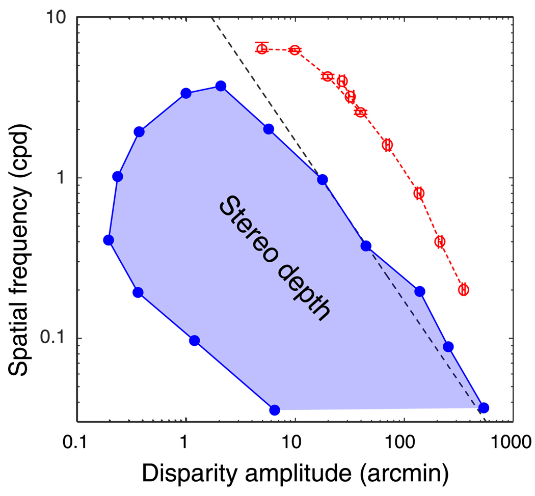
The boundary on the top-right and top of the stereo depth region in Figure 1 represents the disparity-gradient limit and stereoresolution limit. We have shown here that the local cross-correlation model exhibits both phenomena. If this is the case, the model should have constraints in the combinations of disparity amplitude and spatial frequency like the ones in Figure 1. To examine this, we constructed an orientation-discrimination task similar to the one used in the Stereoresolution section of this paper and presented it to the model. A random-dot stereogram defined a disparity-modulated sine wave rotated ±10° from horizontal. For the right part of the depth region in Figure 1, spatial frequency was fixed and the disparity amplitude threshold was measured. For the top part of the depth region, amplitude was fixed and the spatial-frequency threshold was found. Figure 20 shows the modeling results (red points) along with Tyler’s data from human observers. As we expected, the model’s fusion limit in the upper right falls on a line with a slope of −1; this is very similar to Tyler’s results except for the fact that the model can handle larger disparities in part because it is not penalized for off-horopter disparity estimates. The model’s stereoresolution levels off at ~6 cpd, a bit higher than the human asymptote. The human data and model data are therefore quite similar in shape except for the model’s generally higher sensitivity.

Figure 20.

Combinations of disparity amplitude and spatial frequency that yield depth percepts. The filled points are data replotted from Tyler (1975). The shaded region represents the combinations of disparity amplitude and spatial frequency that produce stereoscopic depth percepts. The unshaded region represents combinations that do not yield such percepts. The red points are the modeling results. The points in the upper right were generated by running an orientation-discrimination task (±10°) with disparity-defined sine waves. Spatial frequency was fixed, and the maximum disparity amplitude yielding 75% correct performance was determined. The points at the top were generated in the same way except that disparity amplitude was fixed and the spatial-frequency threshold was determined. Dot density was 300 dots/deg² and window size was 6 arcmin. Along the black dashed line, the product of spatial frequency and disparity is constant.

We showed that the disparity-gradient limit and stereoresolution can both be understood as consequences of using local cross-correlation to estimate disparity. Thus, these limitations of human stereopsis are byproducts of the method used for disparity estimation.

References

- Akerstrom RA, Todd JT. The perception of stereoscopic transparency. Perception & Psychophysics. 1988;44:421–432. doi: 10.3758/bf03210426. [PubMed] [DOI] [PubMed] [Google Scholar]
- Anzai A, Ohzawa I, Freeman RD. Neural mechanisms for processing binocular information. I. Simple cells. Journal of Neurophysiology. 1999;82:891–908. doi: 10.1152/jn.1999.82.2.891. [PubMed] [Article] [DOI] [PubMed] [Google Scholar]
- Arnold R, Binford T. Geometric constraints on stereo vision. Proceedings of SPIE. 1980;238:281–292. [Google Scholar]
- Backus BT, Banks MS, van Ee R, Crowell JA. Horizontal and vertical disparity, eye position, and stereoscopic slant perception. Vision Research. 1999;39:1143–1170. doi: 10.1016/s0042-6989(98)00139-4. [PubMed] [DOI] [PubMed] [Google Scholar]
- Banks MS, Geisler WS, Bennett PJ. The physical limits of grating visibility. Vision Research. 1987;27:1915–1924. doi: 10.1016/0042-6989(87)90057-5. [PubMed] [DOI] [PubMed] [Google Scholar]
- Banks MS, Gepshtein S, Landy MS. Why is spatial stereoresolution so low? Journal of Neuroscience. 2004;24:2077–2089. doi: 10.1523/JNEUROSCI.3852-02.2004. [PubMed] [Article] [DOI] [PMC free article] [PubMed] [Google Scholar]
- Banks MS, Sekuler AB, Anderson SJ. Peripheral spatial vision: Limits imposed by optics, photoreceptors, and receptor pooling. Journal of the Optical Society of America A, Optics and Image Science. 1991;8:1775–1787. doi: 10.1364/josaa.8.001775. [PubMed] [DOI] [PubMed] [Google Scholar]
- Blakemore C. The range and scope of binocular depth discrimination in man. The Journal of Physiology. 1970;211:599–622. doi: 10.1113/jphysiol.1970.sp009296. [PubMed] [Article] [DOI] [PMC free article] [PubMed] [Google Scholar]
- Bradshaw MF, Rogers BJ. Sensitivity to horizontal and vertical corrugations defined by binocular disparity. Vision Research. 1999;39:3049–3056. doi: 10.1016/s0042-6989(99)00015-2. [PubMed] [DOI] [PubMed] [Google Scholar]
- Burt P, Julesz B. A disparity gradient limit for binocular fusion. Science. 1980;208:615–617. doi: 10.1126/science.7367885. [PubMed] [DOI] [PubMed] [Google Scholar]
- Campbell FW, Robson JG. Application of Fourier analysis to the visibility of gratings. The Journal of Physiology. 1968;197:551–566. doi: 10.1113/jphysiol.1968.sp008574. [PubMed] [Article] [DOI] [PMC free article] [PubMed] [Google Scholar]
- Clerc M, Mallat S. The texture gradient equation for recovering shape from texture. IEEE Transactions on Pattern Analysis and Machine Intelligence. 2002;24:536–549. [Google Scholar]
- Cormack LK, Stevenson SB, Schor CM. Interocular correlation, luminance contrast and cyclopean processing. Vision Research. 1991;31:2195–2207. doi: 10.1016/0042-6989(91)90172-2. [PubMed] [DOI] [PubMed] [Google Scholar]
- Cumming BG, DeAngelis GC. The physiology of stereopsis. Annual Review of Neuroscience. 2001;24:203–238. doi: 10.1146/annurev.neuro.24.1.203. [PubMed] [DOI] [PubMed] [Google Scholar]
- Fleet DJ, Wagner H, Heeger DJ. Neural encoding of binocular disparity: Energy models, position shifts and phase shifts. Vision Research. 1996;36:1839–1857. doi: 10.1016/0042-6989(95)00313-4. [PubMed] [DOI] [PubMed] [Google Scholar]
- Geisler WS, Davila KD. Ideal discriminators in spatial vision: Two-point stimuli. Journal of the Optical Society of America A, Optics and Image Science. 1985;2:1483–1497. doi: 10.1364/josaa.2.001483. [PubMed] [DOI] [PubMed] [Google Scholar]
- Harris JM, McKee SP, Smallman HS. Fine-scale processing in human binocular stereopsis. Journal of the Optical Society of America A, Optics, Image Science, and Vision. 1997;14:1673–1683. doi: 10.1364/josaa.14.001673. [PubMed] [DOI] [PubMed] [Google Scholar]
- Held R, Banks MS. Misperceptions in stereoscopic displays: A vision science perspective. ACM Transactions. 2008;APGV08:23–31. doi: 10.1145/1394281.1394285. [DOI] [PMC free article] [PubMed] [Google Scholar]
- Hillis JM, Banks MS. Are corresponding points fixed? Vision Research. 2001;41:2457–2473. doi: 10.1016/s0042-6989(01)00137-7. [PubMed] [DOI] [PubMed] [Google Scholar]
- Hillis JM, Watt SJ, Landy MS, Banks MS. Slant from texture and disparity cues: Optimal cue combination. Journal of Vision. 2004;4(12):967–992. doi: 10.1167/4.12.1. 1 http://journalofvision.org/4/12/1/, doi:10.1167/4.12.1. [PubMed] [Article] [DOI] [PubMed] [Google Scholar]
- Kanade T, Okutomi M. A stereo matching algorithm with an adaptive window: Theory and experiment. Proceedings of the IEEE International Conference on Robotics and Automation. 1994;16:920–932. [Google Scholar]
- Levi DM, Klein SA. Vernier acuity, crowding and amblyopia. Vision Research. 1985;25:979–991. doi: 10.1016/0042-6989(85)90208-1. [PubMed] [DOI] [PubMed] [Google Scholar]
- Li Z, Hu G. Analysis of disparity gradient based cooperative stereo. IEEE Transactions on Image Processing. 1996;5:1493–1506. doi: 10.1109/83.541420. [DOI] [PubMed] [Google Scholar]
- MacLeod DI, Williams DR, Makous W. A visual nonlinearity fed by single cones. Vision Research. 1992;32:347–363. doi: 10.1016/0042-6989(92)90144-8. [PubMed] [DOI] [PubMed] [Google Scholar]
- Marr D, Poggio T. Cooperative computation of stereo disparity. Science. 1976;194:283–287. doi: 10.1126/science.968482. [PubMed] [DOI] [PubMed] [Google Scholar]
- McKee SP, Verghese P. Stereo transparency and the disparity gradient limit. Vision Research. 2002;42:1963–1977. doi: 10.1016/s0042-6989(02)00073-1. [PubMed] [DOI] [PubMed] [Google Scholar]
- Nguyenkim JD, DeAngelis GC. Disparity-based coding of three-dimensional surface orientation by macaque middle temporal neurons. Journal of Neuroscience. 2003;23:7117–7128. doi: 10.1523/JNEUROSCI.23-18-07117.2003. [PubMed] [Article] [DOI] [PMC free article] [PubMed] [Google Scholar]
- Nienborg H, Bridge H, Parker AJ, Cumming BG. Receptive field size in V1 neurons limits acuity for perceiving disparity modulation. Journal of Neuroscience. 2004;24:2065–2076. doi: 10.1523/JNEUROSCI.3887-03.2004. [PubMed] [Article] [DOI] [PMC free article] [PubMed] [Google Scholar]
- Ogle KN. Precision and validity of stereoscopic depth perception from double images. Journal of the Optical Society of America. 1953;43:907–913. doi: 10.1364/josa.43.000906. [PubMed] [DOI] [PubMed] [Google Scholar]
- Ohzawa I. Mechanisms of stereoscopic vision: The disparity energy model. Current Opinions in Neurobiology. 1998;8:509–515. doi: 10.1016/s0959-4388(98)80039-1. [PubMed] [DOI] [PubMed] [Google Scholar]
- Ohzawa I, DeAngelis GC, Freeman RD. Stereoscopic depth discrimination in the visual cortex: Neurons ideally suited as disparity detectors. Science. 1990;249:1037–1041. doi: 10.1126/science.2396096. [PubMed] [DOI] [PubMed] [Google Scholar]
- Panton D. A flexible approach to digital stereo mapping. Photogrammetric Engineering & Remote Sensing. 1978;44:1499–1512. [Google Scholar]
- Panum PL. Physiologische untersuchungen über das sehen mit zwei augen. Kiel, Germany: Schwers; 1858. [Google Scholar]
- Pollard SB, Mayhew JE, Frisby JP. PMF: A stereo correspondence algorithm using a disparity gradient limit. Perception. 1985;14:449–470. doi: 10.1068/p140449. [PubMed] [DOI] [PubMed] [Google Scholar]
- Porrill J, Mayhew J, Frisby J. Frontiers of visual science: Proceedings of the 1985 Symposium. Washington, DC: National Academy Press; 1985. Cyclotorsion, conformal invariance, and induced effects in stereoscopic vision; pp. 90–108. [Google Scholar]
- Prazdny K. Detection of binocular disparities. Biological Cybernetics. 1985;52:93–99. doi: 10.1007/BF00363999. [PubMed] [DOI] [PubMed] [Google Scholar]
- Prince SJ, Eagle RA. Stereo correspondence in one-dimensional Gabor stimuli. Vision Research. 2000;40:913–924. doi: 10.1016/s0042-6989(99)00242-4. [PubMed] [DOI] [PubMed] [Google Scholar]
- Rogers BJ, Bradshaw MF. Vertical disparities, differential perspective and binocular stereopsis. Nature. 1993;361:253–255. doi: 10.1038/361253a0. [PubMed] [DOI] [PubMed] [Google Scholar]
- Rogers BJ, Bradshaw MF. Disparity scaling and the perception of frontoparallel surfaces. Perception. 1995;24:155–179. doi: 10.1068/p240155. [PubMed] [DOI] [PubMed] [Google Scholar]
- Shikata E, Tanaka Y, Nakamura H, Taira M, Sakata H. Selectivity of the parietal visual neurones in 3D orientation of surface of stereoscopic stimuli. Neuroreport. 1996;7:2389–2394. doi: 10.1097/00001756-199610020-00022. [PubMed] [DOI] [PubMed] [Google Scholar]
- Stevens KA. Representing and analyzing surface orientation. In: Winston PH, Brown RH, editors. Artificial intelligence: An MIT perspective. Cambridge, MA: MIT Press; 1979. pp. 104–125. [Google Scholar]
- Stevenson SB, Cormack LK, Schor CM, Tyler CW. Disparity tuning in mechanisms of human stereopsis. Vision Research. 1992;9:1685–1694. doi: 10.1016/0042-6989(92)90161-b. [PubMed] [DOI] [PubMed] [Google Scholar]
- Trivedi HP, Lloyd SA. The role of disparity gradient in stereo vision. Perception. 1985;14:685–690. doi: 10.1068/p140685. [PubMed] [DOI] [PubMed] [Google Scholar]
- Tyler CW. Stereoscopic vision: Cortical limitations and a disparity scaling effect. Science. 1973;181:276–278. doi: 10.1126/science.181.4096.276. [PubMed] [DOI] [PubMed] [Google Scholar]
- Tyler CW. Depth perception in disparity gratings. Nature. 1974;251:140–142. doi: 10.1038/251140a0. [PubMed] [DOI] [PubMed] [Google Scholar]
- Tyler CW. Spatial organization of binocular disparity sensitivity. Vision Research. 1975;15:583–590. doi: 10.1016/0042-6989(75)90306-5. [PubMed] [DOI] [PubMed] [Google Scholar]
- Watson AB. Frontiers of visual science: Proceedings of the 1985 Symposium. Washington, DC: National Academy Press; 1985. The ideal observer concept as a modeling tool. [Google Scholar]
- Watson AB, Barlow HB, Robson JG. What does the eye see best? Nature. 1983;302:419–422. doi: 10.1038/302419a0. [PubMed] [DOI] [PubMed] [Google Scholar]
- Wichmann FA, Hill NJ. The psychometric function: I. Fitting, sampling, and goodness of fit. Perception & Psychophysics. 2001;63:1293–1313. doi: 10.3758/bf03194544. [PubMed] [DOI] [PubMed] [Google Scholar]
- Ziegler LR, Hess RF, Kingdom FA. Global factors that determine the maximum disparity for seeing cyclopean surface shape. Vision Research. 2000;40:493–502. doi: 10.1016/s0042-6989(99)00206-0. [PubMed] [DOI] [PubMed] [Google Scholar]