Symmetry Breakdown in the ON and OFF Pathways of the Retina at Night: Functional Implications

Abstract

Several recent studies have shown that the ON and OFF channels of the visual system are not simple mirror images of each other, that their response characteristics are asymmetric (Chichilnisky and Kalmar, 2002; Sagdullaev and McCall, 2005). How the asymmetries bear on visual processing is not well understood. Here, we show that ON and OFF ganglion cells show a strong asymmetry in their temporal adaptation to photopic (day) and scotopic (night) conditions and that the asymmetry confers a functional advantage. Under photopic conditions, the ON and OFF ganglion cells show similar temporal characteristics. Under scotopic conditions, the two cell classes diverge—ON cells shift their tuning to low temporal frequencies, whereas OFF cells continue to respond to high. This difference in processing corresponds to an asymmetry in the natural world, one produced by the Poisson nature of photon capture and persists over a broad range of light levels. This work characterizes a previously unknown divergence in the ON and OFF pathways and its utility to visual processing. Furthermore, the results have implications for downstream circuitry and thus offer new constraints for models of downstream processing, since ganglion cells serve as building blocks for circuits in higher brain areas. For example, if simple cells in visual cortex rely on complementary interactions between the two pathways, such as push–pull interactions (Alonso et al., 2001; Hirsch, 2003), their receptive fields may be radically different under scotopic conditions, when the ON and OFF pathways are out of sync.

Introduction

The ON and OFF pathways are among the most well known examples of parallel processing in the visual system (Wässle, 2004). The division into these streams begins in the retina at the very first synapse—bipolar cells contain either sign-inverting or sign-conserving glutamate receptors, which determine whether they depolarize or hyperpolarize to light. The depolarizing and hyperpolarizing bipolar cells constitute two general classes of cells, termed ON and OFF bipolar cells. The ON and OFF bipolar cells send their axon terminals to separate sublaminae in the inner-plexiform layer, where they synapse with ganglion cell dendrites and shape ganglion cell responses. Thus, the split into cells that respond to ON and OFF signals in the retina is carried forth from the first synapse to the ganglion cell output.

Initially, the working hypothesis was that this ON and OFF output was essentially “equal and opposite,” that is, the ON and OFF cells were thought to respond to the same features of the visual scene, just with opposite polarity. Evidence has begun to accumulate, however, that this description is too simple, that ON and OFF cells carry at least partially different information. Specifically, at the level of the retinal circuitry, studies have shown that the two pathways receive distinct inhibitory input (Pang et al., 2003; Zaghloul et al., 2003; Murphy and Rieke, 2006; Eggers et al., 2007; Molnar and Werblin, 2007). Furthermore, at the level of retinal output, ON and OFF cells of the same class have been shown to have 10–20% differences in receptive field size and kinetics (Chichilnisky and Kalmar, 2002) (but see Benardete and Kaplan, 1999, with respect to the kinetics), and additional differences in the degree of nonlinearity (Sagdullaev and McCall, 2005). The significance of these differences for visual processing is not well understood. Although a proposal has been made for the functional role of the difference in receptive field size (a spatial aspect) (Balasubramanian and Sterling, 2009), the roles of the differences in dynamics have yet to be determined.

Here, we show that ON and OFF cells show a substantial difference in their temporal adaptation to day and night, and, furthermore, that this difference has a functional advantage. We characterized the temporal responses of mouse ON and OFF ganglion cells using gratings and white-noise stimuli under photopic and scotopic conditions. Our results show that under photopic conditions, the pathways are, in fact, largely symmetric: their responses differ in sign, but their temporal characteristics are similar. Under scotopic conditions, however, the pathways diverge—the tuning of the ON cells shifts to low temporal frequencies, whereas the tuning of the OFF cells remains high. Using a model for signal detection, we then address the issue at the functional level, showing how this difference corresponds to a natural asymmetry in the visual world.

These results show a new divergence in the ON and OFF pathways and its potential value for processing visual information. The results also have implications for downstream circuitry, specifically, for receptive field models that depend on ON and OFF interactions.

Materials and Methods

Experiments

Recording.

Ganglion cell spike trains were recorded from the central retina of C57BL/6J mice using a multielectrode array, as described previously (Nirenberg et al., 2001; Sinclair et al., 2004; Dedek et al., 2008). Spikes were sorted into units (cells) using a Plexon Instruments Multichannel Neuronal Acquisition Processor. Five retinas were used in these studies. Retina pieces used for the recordings were ∼1.5–2 mm across.

Stimulation.

The light source for these experiments was a Sony Multiscan CPD-15SX1 computer monitor. Neutral density filters were used to attenuate the output of the monitor to the desired scotopic and photopic levels. The scotopic intensity was 2.8 × 10⁻⁵ μW/cm²; the photopic was 0.25 μW/cm². Following Lyubarsky et al. (2004) and using the spectrum of our monitor (Bohnsack et al., 1997), these radiometric units can be converted to photoreceptor-equivalent-photons · micrometers⁻² · second⁻¹: The scotopic intensity converts to 0.3 rod-equivalent-photons · μm⁻² · s⁻¹, 0.3 M-cone-equivalent-photons · μm⁻² · s⁻¹ [in mouse, the rod and the M-cone have very closely matching absorption spectra (Lyubarsky et al., 1999; Nirenberg et al., 2001)], and 0.01 S-cone-equivalent-photons · μm⁻² · s⁻¹, the photopic, to 2.7 × 10³ rod-equivalent-photons · μm⁻² · s⁻¹, 2.7 × 10³ M-cone-equivalent-photons · μm⁻² · s⁻¹, and 120 S-cone-equivalent-photons · μm⁻² · s⁻¹. This gives a rate of 0.2 R* · rod⁻¹ · s⁻¹, 0.1 R* · M-cone⁻¹ · s⁻¹, and 5 × 10⁻³ R* · S-cone⁻¹ · s⁻¹ for scotopic, and 1.8 × 10³ R* · rod⁻¹ · s⁻¹, 900 R* · M-cone⁻¹ · s⁻¹, and 40 R* · S-cone⁻¹ · s⁻¹ for photopic, assuming an effective collecting area (i.e., collecting area/funneling factor) from the studies by Lyubarsky et al. (1999, 2004) of 0.67 μm² for rods and 0.34 μm² for cones. Note that recordings were made in central retina, where most cones coexpress both opsins (Applebury et al., 2000; Nikonov et al., 2006). Thus the numbers 900 R* · cone⁻¹ · s⁻¹ and 40 R* · cone⁻¹ · s⁻¹ constitute the range of photoisomerizations at the higher light intensity. See also supplemental material (available at www.jneurosci.org) for experiments with 2-amino-4-phosphonobutyric acid (APB) that show that responses to the low light level condition are mediated through the rod bipolar pathway.

Two stimuli were used: drifting sine wave gratings and a binary random checkerboard (white noise). The sine wave gratings were presented at nine temporal frequencies, ranging from 0.15 to 6 Hz, all with a spatial frequency of 0.039 cycles/deg. Each temporal frequency was presented for 2 min. The white noise stimulus was a random checkerboard at a contrast of 1, in which the intensity of each square was either white or black, randomly chosen every 0.067 s. The size of the squares was 9 × 9°; this size was chosen to elicit responses in the low-light (scotopic) condition. The white noise stimulus was presented for 10 min. Note that the update rate of the white noise stimulus, 1/0.067 = 15 Hz, which would be considered low for some species, is appropriate for the mouse, the responses of whose ganglion cells fall off rapidly above 5 Hz. The frequency range focused on in this paper is 3–0.5 Hz (or lower). With a noise update rate of 15 Hz and a corresponding Nyquist frequency of 7.5 Hz, this range is well covered. After both stimuli were presented, the light intensity was increased. After 20 min of adaptation to the photopic intensity, the stimuli were presented again, as above. All animals were dark-adapted for 1 h before recording.

Assessing potential rundown caused by bleaching.

Response rundown can occur because of bleaching during the photopic condition. To assess this, we measured the firing rate in the responses to a periodic flashing stimulus at the beginning and end of the photopic condition. Firing rates between the beginning and end differed by <10% on average, and this was not significantly different between ON and OFF cells (p > 0.5, Student's t test comparing the mean firing rate change of ON cells with that of the OFF cells).

Data analysis

Designation of ON and OFF cells.

Cells were designated as ON or OFF using the spike-triggered average to the checkerboard stimulus (see above). If the sign of the initial deflection was positive, the cells were designated as ON, and if negative, then OFF.

Analysis of responses to drifting gratings.

For the drifting sine wave gratings, temporal tuning curves were created from ganglion cell responses using standard methods (Enroth-Cugell and Robson, 1966; Purpura et al., 1990; Croner and Kaplan, 1995). Briefly, for each grating, the first harmonic of the response of the cell, R(f), was calculated as follows:

where f is the temporal frequency of the drifting sine wave grating (in cycles/second), L is the duration of the stimulus (in seconds), which was always an integer multiple of 1/f, and t_j is the time of the jth spike of the response of the cell to the given grating.

Analysis of responses to the white noise stimulus.

For the white noise stimulus, spike-triggered averages were computed using reverse correlation (for review, see Chichilnisky, 2001). When calculating temporal frequency responses, for a given cell, the input stimulus was the intensity of the checkerboard square that produced the largest response for that cell. Temporal frequency responses were then taken as the transfer function between that stimulus and the response of the cell, calculated as follows:

where f is the temporal frequency of interest, W_XY is the cross-spectrum between the stimulus and response, and W_XX is the power spectrum of the stimulus. Spectra were estimated using the multitaper method [Chronux library for Matlab (Mitra and Bokil, 2007); available at http://chronux.org], using an effective bandwidth of 0.27 Hz.

Generation of confusion matrices.

Confusion matrices were used to quantify and visualize the extent to which different stimuli could be distinguished based on the ganglion cell responses. The vertical axis of a confusion matrix gives the presented stimulus (i), whereas the horizontal axis gives the decoded stimulus (j). Each element (i,j) of the confusion matrix indicates the probability that when stimulus i is presented, it will be decoded as stimulus j. The matrices were constructed using the responses to the drifting sine wave grating stimuli at the seven highest temporal frequencies, ranging from 0.45 to 6 Hz (the extreme low-frequency gratings did not provide a sufficient number of repeats for estimating probability distributions and thus were not included in the construction of the matrices).

On each trial of the task, a stimulus, s, was presented (a grating of a particular temporal frequency), and a response, r, was recorded. The response was then decoded by choosing the stimulus most likely to have produced it. The probability that a recorded response r is produced by the stimulus s_j, namely, p(s_j|r), can be calculated by Bayes rule as follows:

Thus, to decode a response r, we need to find the stimulus s_j for which p(r|s_j) is maximal. (This is because all stimuli were equally likely [i.e., all p(s_j) are identical].)

To calculate the response distribution for each stimulus, p(r|s_j), we proceeded as follows. First, the 34 trials at each frequency were split into interleaved sets: one set to build the response distributions (the training set) and the other set to be decoded (the test set). For each stimulus, the response distribution was assumed to be an inhomogenous Poisson process spanning 1.2 s, and constant in 133 ms bins. The firing rate in each bin was estimated by binning each spike train at this resolution, and averaging over all training trials of a given stimulus. To calculate p(r|s_j) for a response in the test set, we binned responses in the same manner. Since we assumed that the conditional response distribution is an inhomogeneous Poisson process, the probability p(r|s_j) was the product of the Poisson probabilities for each bin. This process was repeated for each response in the test set, and results were tallied into the confusion matrix. Results similar to those shown in Figures 5 and 6 were obtained with a range of bin sizes (75–170 ms) and random assignments to training and test sets.

Figure 5.

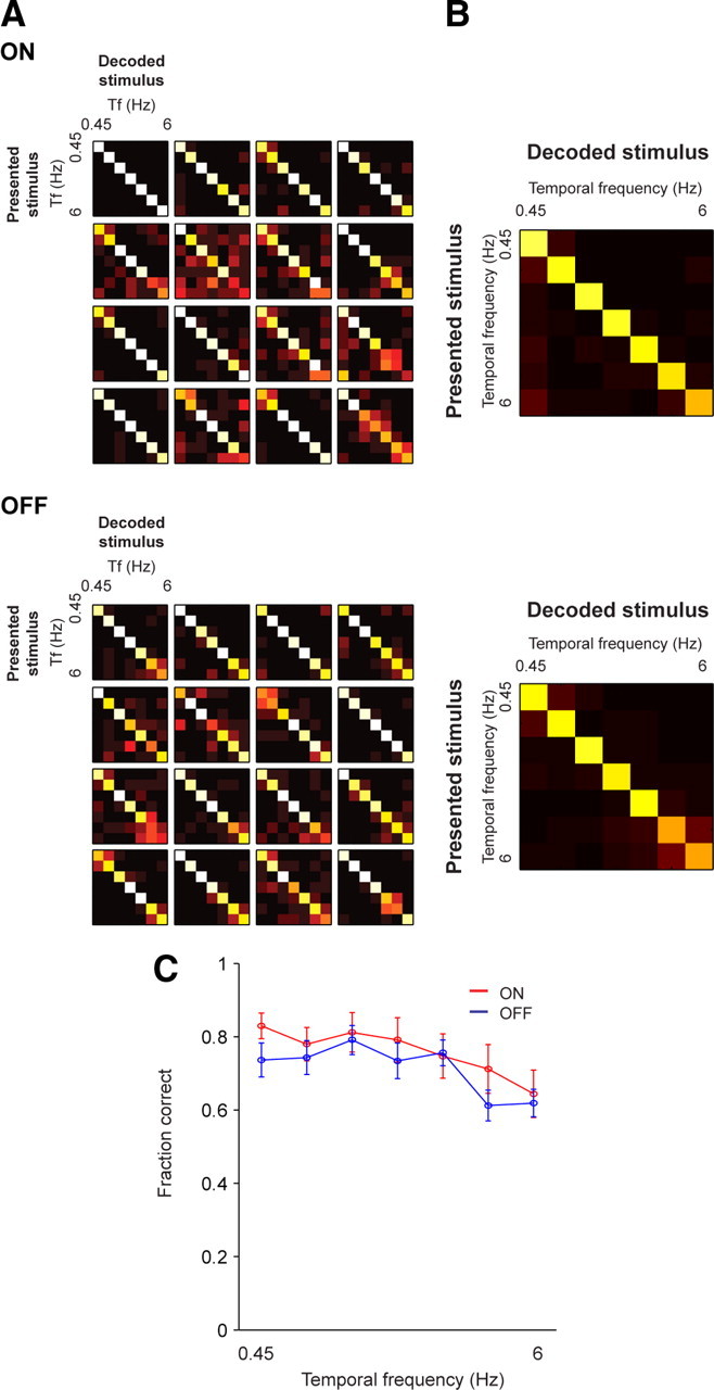
Under photopic conditions, it is possible to decode across the entire range of temporal frequencies using responses of ON or OFF cells. A, Representative confusion matrices for 16 ON and 16 OFF cells calculated using responses to drifting gratings. The vertical axis gives the presented stimulus (i), and the horizontal axis gives the decoded stimulus (j). Each element of a confusion matrix plots the probability of decoding stimulus j when presented with stimulus i (see text). Decoders based on both ON and OFF responses show little confusion over the range of temporal frequencies, as indicated by the prominent diagonal lines in the confusion matrices. B, Average confusion matrices over all ON and OFF cells (n = 20 ON cells; n = 31 OFF cells). C, The average of the diagonals of the matrices (mean ± SEM) for all ON (red) and OFF (blue) cells (n = 20 ON cells; n = 31 OFF cells). ON and OFF cells perform equally well over the full range of temporal frequencies (p > 0.1 for all frequencies, Student's t test, adjusted for multiple comparisons).

Figure 6.

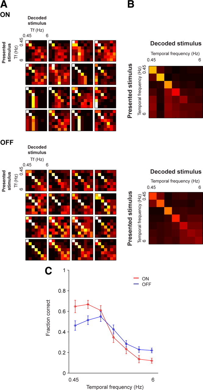
Under scotopic conditions, there is a divergence in performance—ON cells perform better at low frequencies, whereas OFF cells perform better at high. A, Representative confusion matrices calculated using the responses of 16 ON and 16 OFF cells to drifting gratings. ON cells show better performance at low frequencies, as indicated by the bright squares along the diagonal at low frequencies, which break down at middle and high frequencies. In contrast, for OFF cells, performance is shifted toward high frequencies. B, Average confusion matrices over all ON and OFF cells show the same trend (n = 20 ON cells; n = 31 OFF cells). C, The average of the diagonals of the matrices (mean ± SEM) for ON (red) and OFF (blue) populations (n = 20 ON cells; n = 31 OFF cells). ON cells perform significantly better at the lowest two frequencies tested (p < 0.01), whereas OFF cells perform significantly better at the highest frequency (p < 0.01, Student's t test, adjusted for multiple comparisons).

Animals

Animals were from a C57BL/6J background. All experiments were conducted in accordance with the institutional guidelines for animal welfare. Mice were dark-adapted for 1 h before the start of an experiment.

Supplemental material

The supplemental material (available at www.jneurosci.org) provides all individual grating responses, tuning curves, and confusion matrices in the dataset. The figures in the main text show representative examples as well as averages; the supplemental material provides the complete set for the interested reader. The supplemental material also includes a set of figures showing responses after APB application.

Results

To assess differences in the temporal response properties of ON and OFF ganglion cells, we recorded the spiking activity of the cells in response to drifting sine wave gratings of different temporal frequencies and a white noise stimulus. Measurements were performed under both photopic and scotopic conditions.

Figure 1 shows the results for the grating stimulus under the photopic conditions. The left panel shows the responses of several individual ON cells (top) and OFF cells (bottom), and the right panel shows the average temporal frequency tuning curves for the ON and OFF populations (n = 20 ON cells; n = 31 OFF cells). Consistent with previous studies (Kremers et al., 1993; Benardete and Kaplan, 1999; Keat et al., 2001; Zaghloul et al., 2003), both cell classes responded similarly, that is, they both responded to a broad range of temporal frequencies (0.15–6 Hz) (p > 0.05, Student's t test comparing the mean center of mass of the ON cell tuning curves with those of the OFF cells).

Figure 1.

ON and OFF cells show similar temporal frequency tuning in response to sine wave gratings under photopic conditions. A, Representative responses for four ON and four OFF ganglion cells to drifting sine wave gratings of increasing temporal frequency. Each segment of the traces shows the average firing rate over one period of the drifting grating for a given frequency. B, Average tuning curves (mean ± SEM) for all ON and OFF cells, normalized to the peak (n = 20 ON cells, 31 OFF cells). Temporal tuning curves were calculated by Fourier analyzing the responses and extracting the amplitude of the first harmonic response at each frequency. ON and OFF cells respond to a similar range of temporal frequencies (p > 0.05, Student's t test, comparing the mean center of mass of the ON cell tuning curves with that of the OFF cells).

The results for the same cells under scotopic conditions are shown in Figure 2. As in Figure 1, the left panel shows responses for several individual ON and OFF cells, and the right panel shows the average tuning curves. In contrast to the photopic condition, there was a clear difference in tuning: ON cells showed tuning to low temporal frequencies, peaking near 0.5 Hz, whereas OFF cells continued to respond to high temporal frequencies. The difference in tuning between the ON and OFF populations was highly significant (p < 10⁻³, Student's t test, comparing the mean center of mass of the tuning curves of the two populations).

Figure 2.

Frequency tuning of ON and OFF cells diverges under scotopic conditions. A, Representative responses of four ON and four OFF ganglion cells to drifting sine wave gratings of increasing temporal frequency. B, Average tuning curves (mean ± SEM) for all ON and OFF cells, normalized to the peak (n = 20 ON cells, 31 OFF cells). On average, the ON cells shifted to low frequencies, whereas the OFF cells continued to respond to high frequencies (p < 10⁻³, Student's t test, comparing the mean center of mass of the two populations). Note that, under scotopic conditions, both ON and OFF cells fail to respond to the extreme high frequencies.

Similar results occurred for the white noise stimulus (Figs. 3, 4). Figure 3 shows the responses from the two cell classes under photopic conditions. The left panel shows the time course of the spike-triggered average (STA) for several ON cells and OFF cells, and the right panel shows the average temporal frequency responses for both cell classes (n = 20 ON cells, 31 OFF cells). As with the grating stimulus, both cell types responded similarly over a broad range of temporal frequencies (p > 0.05, Student's t test, comparing the mean center of mass of the ON cell temporal frequency responses with those of the OFF cells). Figure 4 shows the responses to the same stimulus under scotopic conditions. Again, the left panel shows STA time courses for individual ON and OFF cells, and the right panel shows the average temporal frequency responses across all cells for the two populations. The same divergence in tuning observed with the grating stimulus—that ON cells were tuned to low frequencies, whereas OFF cells continued to respond to high frequencies—was also seen with the white noise stimulus (p < 10⁻³, Student's t test, comparing the mean center of mass of the temporal frequency responses of the two populations).

Figure 3.

ON and OFF cells show similar temporal response properties to white noise under photopic conditions. A, Representative STA time courses for four ON and four OFF ganglion cells in response to a white noise (random checkerboard) stimulus. Note that OFF STAs are inverted so that the similarity of the short peaks is easy to observe. B, Average temporal frequency responses (mean ± SEM) for all ON and OFF cells (n = 20 ON cells, n = 31 OFF cells), normalized to the peak. Temporal frequency responses were calculated by Fourier analyzing the STA at the checkerboard square that produced the largest response for each cell. ON and OFF cells showed similar temporal response profiles (p > 0.05, Student's t test, comparing the mean center of mass of ON cell temporal frequency responses with that of the OFF cells).

Figure 4.

The divergence under scotopic conditions was also observed for the white noise stimulus. A, Representative STA time courses for four ON and four OFF ganglion cells in response to a white noise (random checkerboard) stimulus. B, Average temporal frequency responses (mean ± SEM), normalized to the peak (n = 20 ON cells, n = 31 OFF cells). As with the grating stimulus, the ON cells shifted to low frequencies, whereas the OFF cells continued to respond to high frequencies (p < 10⁻³, Student's t test, comparing the mean center of mass the two populations).

These differences in temporal frequency characteristics show that there is an ON cell/OFF cell asymmetry with respect to encoding stimuli at low light levels. To assess the effects of this on decoding, rather than encoding, stimuli, we used an ideal observer approach (Barlow, 1978; Geisler, 1989). Specifically, we measured the extent to which different stimuli can be distinguished given responses from each cell class.

The decoding results were then quantified and visualized via confusion matrices (Figs. 5, 6) (Hand, 1981). A confusion matrix indicates the probability that the neural response to a presentation of a stimulus will be decoded as that stimulus, or whether it will be confused with another stimulus. Specifically, the element in position (i,i) of the matrix indicates the probability that stimulus i is decoded correctly, and the element in position (i,j) indicates the probability that stimulus i is decoded incorrectly as stimulus j.

Figure 5 shows the confusion matrices generated from responses taken under photopic conditions. The stimuli were drifting gratings of different temporal frequencies. As shown in the figure, both ON and OFF cells decoded the gratings correctly over the range of frequencies; this is indicated by the prominent diagonal line in each confusion matrix. As in the previous figures, results for individual ON and OFF cells are shown on the left, and the average for the population is shown on the right. The results are summarized in B, which shows the average of the diagonals of the matrices for each population (i.e., the average probability that stimuli will be correctly decoded). Under photopic conditions, no statistically significant difference between the classes was observed (p > 0.1 for all frequencies, Student's t test, adjusted for multiple comparisons).

Figure 6 shows the same analysis for these cells under scotopic conditions. Here, there is a clear difference in the decoding: the ON cells showed accurate decoding at low frequencies and poor decoding at high frequencies; this is indicated by the bright squares along the diagonal line at the low frequencies that dissolve as high frequencies are approached. In contrast, the OFF cells showed accurate decoding at high frequencies; here, the bright squares are shifted toward the middle and high frequencies of the matrices. As summarized in B, which shows the average of the diagonals of the matrices for each population, the ON cells were more accurate at low frequencies, whereas the OFF cells were more accurate at high frequencies (p < 0.01, Student's t test, adjusted for multiple comparisons; n = 20 ON cells, n = 31 OFF cells). [All individual grating responses, tuning curves, and confusion matrices for both light conditions are provided in supplemental material for the interested reader (supplemental Fig. S1 for ON cells; supplemental Fig. S2 for OFF cells, available at www.jneurosci.org).]

The above finding—that ON cells but not OFF cells shift to low temporal frequencies in the dark—indicates that, as light level decreases, the retina processes increments and decrements differently. Interestingly, this difference in processing corresponds to an asymmetry in the physical world, one produced by the Poisson nature of photon capture. In a Poisson process, the variance is proportional to the mean. This means that there is more dispersion in the distribution of counts when the event rate increases (i.e., when light increments occur) than when the event rate decreases (when light decrements occur). Because of this asymmetry, more time is needed to detect increments than decrements.

The effect of this asymmetry is shown in Figure 7A. We consider the discrimination of positive and negative fluctuations around a background luminance. As mentioned above, Poisson statistics dictate that increments are associated with broader count distributions, and decrements with narrower ones. Consequently, there is more overlap among the increments, making them harder to distinguish. As shown in B, an ideal observer in a discrimination task, who chooses stimuli based on the maximum a posteriori probability over the set of stimuli, will be less accurate in discriminating between increments than between decrements. Changing the event count (either by changing the integration time or the photon rate) changes performance for both increments and decrements, but the difference between decrements and increments persists—for at least three orders of magnitude, as shown in the figure. (Appendix provides an information-theoretic analysis of this asymmetry.)

Figure 7.

At low light levels, increments become harder to discriminate than decrements of equal magnitude, because of asymmetries in the Poisson distribution. A, Distributions of photon counts are shown for increments (gray) and decrements (black) in steps of 10% contrast around a mean rate (dotted line). For increments, the distributions are broader and show much greater overlap than for decrements, making increments harder to detect. B, Performance for an ideal observer in the discrimination task for increments (gray) or decrements (black) over a range of mean photon counts. For each mean photon count, stimuli at steps of ±10% contrast around the mean are simulated (as in A), and the observer chooses stimuli based on the maximum a posteriori probability over the set of stimuli. Over a broad range of photon counts, performance is better for decrements than for increments. The arrows indicate separation between increment and decrement performance (i.e., the factor by which an increment detector needs to observe more photons to match the performance of the decrement detector). The dotted line indicates performance at chance. We note that this aspect of Poisson processes—that it is more difficult to detect increments than to detect decrements—might seem counterintuitive, since signal-to-noise ratio (SNR) increases with mean rate increases. But SNR is not the relevant statistic here. An increase in SNR means that it is easier to detect the same fractional change around a high mean rate than around a low mean rate. In our case, we are asking whether, given a constant mean rate (e.g., the rate under night conditions), it is easier to detect an increment or a decrement. Since the variability of a Poisson process is proportional to its rate, an increment leads to a more variable signal than a decrement and, therefore, is harder to detect. The suggestion in this paper, then, is that ON cells compensate for the higher variability by integrating their input over a longer period of time (i.e., by shifting toward low temporal frequencies).

Discussion

It is well known that the signals in the first stages of visual processing segregate into ON and OFF channels. The working hypothesis for many years was that these channels are symmetric, but recent observations suggest that this notion needs modification, that the two pathways show differences (Devries and Baylor, 1997; Demb et al., 2001; Chichilnisky and Kalmar, 2002; Pang et al., 2003; Zaghloul et al., 2003; Sagdullaev and McCall, 2005; Murphy and Rieke, 2006; Eggers et al., 2007; Molnar and Werblin, 2007). The significance of the differences in conveying visual information has been unclear.

Here, we showed a case in which the symmetry breakdown between the ON and OFF channels is very apparent, and functional significance can be attributed. By day, that is, under photopic conditions, the temporal tuning of ON and OFF ganglion cells in the mouse retina is very similar, but at night it diverges: ON cells shift to low temporal frequencies, that is, they increase their gain at low temporal frequencies and reduce it at high. Figures 2 and 4 show the changes in gain, and Figure 6 shows an example of the functional consequences: the changes in gain correspond to changes in signal-to-noise ratio, which directly affect performance on a temporal frequency discrimination task. Figure 7 then shows that this result is predicted by an asymmetry in the physical world, specifically, the asymmetric detection of light increments and decrements because of the Poisson nature of photon capture.

This breakdown of symmetry between the two pathways in the dark is unlikely to be specific to the mammalian visual system. Armstrong-Gold and Rieke (2003) recorded from ON and OFF bipolar cells under scotopic conditions in the tiger salamander retina and noted that OFF bipolar cells responded to higher frequency stimuli than ON bipolar cells. Although the salamander appears to have significant differences in the circuitry that mediates rod-driven signals (Yang and Wu, 1997), their findings suggest that the asymmetries in the ON and OFF pathways at low light levels generalize to nonmammals as well.

Functional implications of the differences in visual processing

The results in this paper represent an example of a neural system evolving to match a fundamental property of the natural world—the intrinsic asymmetry in the detection of light increments and decrements that arises from the Poisson nature of photon capture. That there is an asymmetry has been previously noted (Cohn, 1974; Thibos et al., 1979; Hornstein et al., 1999), but the studies considered only the implications for photoreceptor responses, and only in the regimen of low photon counts (<10 per discrimination window). Here, we show that the retina exploits this asymmetry after photoreceptor signals are partitioned into ON and OFF channels. Moreover, we demonstrate that this asymmetry is relevant to much higher photon counts, up to thousands of photons per window in our discrimination task (Fig. 7B).

Two factors make the asymmetry relevant to high counts. First, the asymmetry is greater for large deviations from the mean than for small ones. For example, in Figure 7A, the signals near threshold (the distributions of counts closest to the mean) only show a slight difference between increment and decrement distributions and thus would be nearly equally challenging to discriminate. In contrast, for suprathreshold signals (deviations further from the mean), the increment distributions become broader (less discriminable), whereas the decrement distributions become narrower (more discriminable). (Formally, the intrinsic difference in discriminability of increments and decrements depends in an accelerating fashion on distance from the mean—detailed in Appendix.) Second, the effects of the asymmetry are compounded when one considers not just the detection of a single increment or decrement, but instead the discrimination of multiple increments or decrements around a mean photon count. This latter task is much more closely related to the task the animal's visual system is performing—that is, cells in the retina do not simply signal the presence of an increment or decrement, but their response increases with larger magnitude increments or decrements, and therefore the cells must be able to discriminate multiple levels. Because these levels overlap with one another (more so for increments than decrements, as shown in Fig. 7A), the task becomes harder as multiple contrasts are considered, which makes the asymmetry relevant to higher photon counts.

The results of the simple discrimination task, presented in Figure 7B, suggest that ON cells would need to observe more photons, by approximately a factor of 3, to match the performance of OFF cells (shown by the separation between the gray and black curves). (This is similar to the factor of 2.5 found in Appendix using a formal information-theoretic analysis.) This factor of 3 approximates the shift of the tuning curves along the frequency axis seen in the observed data in Figures 2 and 4. Note, however, that the discriminability of increments and decrements will not always differ by this ratio. This is because Poisson fluctuations in photon count are not the only source of noise. As the signals travel through multiple levels of processing, other noise sources are added. To the extent that these noise sources corrupt increments and decrements equally, they will dilute the intrinsic difference in detectability.

An additional point worth mentioning is that the impact of the increment/decrement asymmetry on signaling by ON and OFF ganglion cells depends on the presence of a nonlinearity, specifically, the well known rectification in the output of ganglion cells in many species, including mouse. If, for example, ON cells and OFF cells were not rectified, they could each signal both increments and decrements. In this scenario, the increment/decrement asymmetry would not have a differential effect on the two classes.

Finally, the results in this paper have implications for downstream circuitry, since retinal outputs serve as building blocks for circuits in higher brain areas. For example, some models of simple cell receptive fields in visual cortex hold that cortical cells are activated in a push–pull manner, with ON and OFF subregions driven by complementary ON and OFF retinal ganglion cell input, relayed through the lateral geniculate nucleus (Alonso et al., 2001; Hirsch, 2003). Our findings predict that, if simple cell receptive fields rely on complementarity of ON and OFF input, their receptive field structure may be radically different at night, when the two pathways are out of sync; alternatively, assuming this model is correct, these cells may have some plasticity (e.g., the ability to differentially filter ON and OFF input), which would allow the cells to preserve their receptive field structure with the shift to scotopic vision.

Relating the differential filtering properties of ON and OFF ganglion cells to retinal circuitry

Our results show, at the level of the ganglion cell output, that ON and OFF pathways have filtering properties that diverge in the dark. This requires elements in retinal circuitry that act separately on ON and OFF signals. Under the scotopic conditions used in this paper, signal transmission to ON and OFF ganglion cells is dominated by the rod bipolar pathway (see supplemental material, available at www.jneurosci.org) (for review of the pathway, see Bloomfield and Dacheux, 2001; Völgyi et al., 2004; Murphy and Rieke, 2006, 2008). Along this pathway, ON and OFF signals first diverge at the output from the AII amacrine cell, which connects to ON cone bipolar cells, OFF cone bipolar cells, and OFF ganglion cells. Here, ON signals are mediated by gap junctions, whereas OFF signals (both to the bipolar and ganglion cells) are mediated by chemical synapses (Kolb and Famiglietti, 1974; Strettoi et al., 1992; Völgyi et al., 2004; Murphy and Rieke, 2008). It has been shown recently that, under these conditions, the synaptic input to ON and OFF ganglion cells is correlated (Murphy and Rieke, 2006, 2008), creating an expectation that the ON and OFF responses would be similar. However, it has also been shown that the two ganglion cell types undergo different filtering with respect to their inputs (Murphy and Rieke, 2006, 2008). In ON cells, excitation is followed by delayed inhibition, in a feedforward manner, whereas in OFF cells, excitation and inhibition occur simultaneously, but with opposite polarity; in this case, the cell is driven to fire in a push–pull manner by a combination of excitation and disinhibition. These different filtering mechanisms are potential mediators of the differences in the output properties between the two pathways. We emphasize, however, that since the ON and OFF pathways have not been completely delineated, it is possible that there are other processes as well that shape response dynamics.

Interestingly, under photopic conditions, in which ON and OFF signals diverge at an earlier point in the circuitry (i.e., at the level of the photoreceptor output to the bipolar cells), one might expect greater divergence between ON and OFF ganglion cell responses. This was not the case for the filtering properties we examined. However, differences between the ON and OFF pathways under photopic conditions have been reported by others in studies of adaptation, specifically, contrast adaptation (Chander and Chichilnisky, 2001; Kim and Rieke, 2001; Wark et al., 2009).

Appendix: Discriminability of increments and decrements in the rate of a Poisson process: an information-theoretic perspective

Here, we analyze the asymmetry in detecting increases and decreases in the rate of a Poisson process, viewed from an information-theoretic perspective. This asymmetry has previously been analyzed from the point of view of signal detection theory and asymptotic expressions for receiver operating curve characteristics (Thibos et al., 1979). The information-theoretic perspective used here leads to a simple, exact result (Eq. 10) that indicates how much more quickly an ideal observer can detect a decrement, versus an increment, in a Poisson process. This ratio depends in an accelerating fashion on the fractional size of the change (i.e., the contrast), and, perhaps surprisingly, is independent of the baseline event rate.

To reach our result, we first need a measure of the discriminability of two Poisson processes, one with rate λ_P from one with rate λ_Q. We will then compare the discriminability of a fractional increase in rate by an amount c [i.e., λ_P = λ_Q(1 + c)] to the discriminability of a fractional decrease by the same amount [i.e., λ_P = λ_Q(1 − c)].

The first step is to define a natural measure of discriminability per unit time. We do this by taking the Kullback–Leibler divergence, which is a standard measure of discriminability for discrete distributions, and extending it to continuous processes. For discrete distributions P and Q, the Kullback–Leibler divergence is given by the following:

This is a natural measure of discriminability because it has the following interpretation: given a random draw from the P distribution, D_KL(P‖Q) is the log-likelihood ratio that this observation arises from the P distribution, versus that it arises from the Q distribution (Latham and Nirenberg, 2005; Cover and Thomas, 2006).

To apply this notion to Poisson processes, we note that for a sequence of independent samples, log-likelihood ratios combine by simple addition. In a Poisson process discretized in small intervals of size Δt, each time step is independent. So the discriminability per unit time, which we denote R_KL(P‖Q), is given by the number of time steps (1/Δt) multiplied by the discriminability within a time step of size Δt. Since this holds for infinitesimal time steps as well as finite ones, we can write the following:

where P_Δt and Q_Δt indicate the Poisson processes P and Q, discretized in time steps of size Δt.

We now calculate this single-time-step discriminability, D_KL(P_Δt‖Q_Δt). With time discretized in steps of size Δt, a Poisson process of rate λ can be approximated as a discrete symbol sequence: the symbol 0 occurs with probability 1 − λΔt, and the symbol 1 occurs with probability λΔt. Thus, in a discretization interval Δt, the discriminability of a Poisson sequence with rate λ_P from one with rate λ_Q is as follows:

where p₀ = 1 − λ_PΔt, p₁ = λ_PΔt, q₀ = 1 − λ_QΔt, q₁ = λ_QΔt. The final term in the above equation represents the contribution of bins with two or more events; their contribution is negligible as the step size Δt approaches zero.

With these substitutions, we find the following:

or

Here, we have used the approximation log(1 + u) = u + O(u²) because we are interested in the limit of a small discretization interval, Δt.

From this, it follows that

which is the discriminability per unit time of a Poisson process with rate λ_P from one with rate λ_Q.

Finally, we want to compare the discriminability of a decrement by a fractional contrast c from the background, with the discriminability of an increment by a fractional contrast c from the same background. We represent the background signal as a Poisson process Q with rate λ, and we represent the decrements and increments as Poisson processes Q⁻ and Q⁺, with rates λ⁻ = λ(1 − c) and λ⁺ = λ(1 + c).

The answer we seek, the ratio of discriminabilities, is $\frac{R_{KL}\left(Q^{-}\Vert Q\right)}{R_{KL}\left(Q^{+}\Vert Q\right)}$. Substituting the above expressions for λ⁺ and λ⁻ in Equation 9 yields the following:

The numerator and denominator of $\frac{R_{KL}\left(Q^{-}\Vert Q\right)}{R_{KL}\left(Q^{+}\Vert Q\right)}$ are proportional to the baseline event rate λ, so the ratio of discriminabilities is independent of λ. That is, the ratio of discriminabilities depends only on contrast and the relative photon rates, but not on the absolute photon rate. This gives the ratio in Equation 10 a universal interpretation: it indicates how much more quickly an ideal observer can reach the same certainty in detecting a decrement of a given contrast, versus detecting an increment.

To understand the qualitative behavior of Equation 10, we consider its Taylor expansion. This begins as follows:

Thus, the asymmetry between detection of increments and decrements an accelerating function of the contrast c (Fig. 8): it is progressively more prominent in the suprathreshold range. At the extreme (c = 1), we find $\frac{R_{KL}\left(Q^{-}\Vert Q\right)}{R_{KL}\left(Q^{+}\Vert Q\right)}=\frac{1}{2\log 2-1}$, ∼2.589. That is, abrupt extinction of a light can be detected ∼2.5 times faster than abrupt doubling.

Figure 8.

Decrements can be detected more readily than increments, and the asymmetry is an accelerating function of contrast. To compare intrinsic discriminability, we use the ratio of Kullback–Leibler distances between a baseline Poisson process, and one whose rate changes by a factor of (1 + c) or (1 − c). This ratio (Eq. 10) has a value of 1 for equal discriminability. Values >1 indicate that decrements are more readily discriminated.

References

- Alonso JM, Usrey WM, Reid RC. Rules of connectivity between geniculate cells and simple cells in cat primary visual cortex. J Neurosci. 2001;21:4002–4015. doi: 10.1523/JNEUROSCI.21-11-04002.2001. [DOI] [PMC free article] [PubMed] [Google Scholar]
- Applebury ML, Antoch MP, Baxter LC, Chun LL, Falk JD, Farhangfar F, Kage K, Krzystolik MG, Lyass LA, Robbins JT. The murine cone photoreceptor: a single cone type expresses both S and M opsins with retinal spatial patterning. Neuron. 2000;27:513–523. doi: 10.1016/s0896-6273(00)00062-3. [DOI] [PubMed] [Google Scholar]
- Armstrong-Gold CE, Rieke F. Bandpass filtering at the rod to second-order cell synapse in salamander (Ambystoma tigrinum) retina. J Neurosci. 2003;23:3796–3806. doi: 10.1523/JNEUROSCI.23-09-03796.2003. [DOI] [PMC free article] [PubMed] [Google Scholar]
- Balasubramanian V, Sterling P. Receptive fields and functional architecture in the retina. J Physiol. 2009;587:2753–2767. doi: 10.1113/jphysiol.2009.170704. [DOI] [PMC free article] [PubMed] [Google Scholar]
- Barlow HB. The efficiency of detecting changes of density in random dot patterns. Vision Res. 1978;18:637–650. doi: 10.1016/0042-6989(78)90143-8. [DOI] [PubMed] [Google Scholar]
- Benardete EA, Kaplan E. Dynamics of primate P retinal ganglion cells: responses to chromatic and achromatic stimuli. J Physiol. 1999;519:775–790. doi: 10.1111/j.1469-7793.1999.0775n.x. [DOI] [PMC free article] [PubMed] [Google Scholar]
- Bloomfield SA, Dacheux RF. Rod vision: pathways and processing in the mammalian retina. Prog Retin Eye Res. 2001;20:351–384. doi: 10.1016/s1350-9462(00)00031-8. [DOI] [PubMed] [Google Scholar]
- Bohnsack DL, Diller LC, Yeh T, Jenness JW, Troy JB. Characteristics of the Sony Multiscan 17se Trinitron color graphic display. Spat Vis. 1997;10:345–351. doi: 10.1163/156856897x00267. [DOI] [PubMed] [Google Scholar]
- Chander D, Chichilnisky EJ. Adaptation to temporal contrast in primate and salamander retina. J Neurosci. 2001;21:9904–9916. doi: 10.1523/JNEUROSCI.21-24-09904.2001. [DOI] [PMC free article] [PubMed] [Google Scholar]
- Chichilnisky EJ. A simple white noise analysis of neuronal light responses. Network. 2001;12:199–213. [PubMed] [Google Scholar]
- Chichilnisky EJ, Kalmar RS. Functional asymmetries in ON and OFF ganglion cells of primate retina. J Neurosci. 2002;22:2737–2747. doi: 10.1523/JNEUROSCI.22-07-02737.2002. [DOI] [PMC free article] [PubMed] [Google Scholar]
- Cohn TE. A new hypothesis to explain why the increment threshold exceeds the decrement threshold. Vision Res. 1974;14:1277–1279. doi: 10.1016/0042-6989(74)90228-4. [DOI] [PubMed] [Google Scholar]
- Cover TM, Thomas JA. Elements of information theory. New York: Wiley; 2006. [Google Scholar]
- Croner LJ, Kaplan E. Receptive fields of P and M ganglion cells across the primate retina. Vision Res. 1995;35:7–24. doi: 10.1016/0042-6989(94)e0066-t. [DOI] [PubMed] [Google Scholar]
- Dedek K, Pandarinath C, Alam NM, Wellershaus K, Schubert T, Willecke K, Prusky GT, Weiler R, Nirenberg S. Ganglion cell adaptability: does the coupling of horizontal cells play a role? PLoS ONE. 2008;3:e1714. doi: 10.1371/journal.pone.0001714. [DOI] [PMC free article] [PubMed] [Google Scholar]
- Demb JB, Zaghloul K, Haarsma L, Sterling P. Bipolar cells contribute to nonlinear spatial summation in the brisk-transient (Y) ganglion cell in mammalian retina. J Neurosci. 2001;21:7447–7454. doi: 10.1523/JNEUROSCI.21-19-07447.2001. [DOI] [PMC free article] [PubMed] [Google Scholar]
- Devries SH, Baylor DA. Mosaic arrangement of ganglion cell receptive fields in rabbit retina. J Neurophysiol. 1997;78:2048–2060. doi: 10.1152/jn.1997.78.4.2048. [DOI] [PubMed] [Google Scholar]
- Eggers ED, McCall MA, Lukasiewicz PD. Presynaptic inhibition differentially shapes transmission in distinct circuits in the mouse retina. J Physiol. 2007;582:569–582. doi: 10.1113/jphysiol.2007.131763. [DOI] [PMC free article] [PubMed] [Google Scholar]
- Enroth-Cugell C, Robson JG. The contrast sensitivity of retinal ganglion cells of the cat. J Physiol. 1966;187:517–552. doi: 10.1113/jphysiol.1966.sp008107. [DOI] [PMC free article] [PubMed] [Google Scholar]
- Geisler WS. Ideal observer theory in psychophysics and physiology. Physica Scripta. 1989;39:153–160. [Google Scholar]
- Hand DJ. Discrimination and classification. Chichester, UK: Wiley; 1981. [Google Scholar]
- Hirsch JA. Synaptic physiology and receptive field structure in the early visual pathway of the cat. Cereb Cortex. 2003;13:63–69. doi: 10.1093/cercor/13.1.63. [DOI] [PubMed] [Google Scholar]
- Hornstein EP, Pope DR, Cohn TE. Noise and its effects on photoreceptor temporal contrast sensitivity at low light levels. J Opt Soc Am A Opt Image Sci Vis. 1999;16:705–717. doi: 10.1364/josaa.16.000705. [DOI] [PubMed] [Google Scholar]
- Keat J, Reinagel P, Reid RC, Meister M. Predicting every spike: a model for the responses of visual neurons. Neuron. 2001;30:803–817. doi: 10.1016/s0896-6273(01)00322-1. [DOI] [PubMed] [Google Scholar]
- Kim KJ, Rieke F. Temporal contrast adaptation in the input and output signals of salamander retinal ganglion cells. J Neurosci. 2001;21:287–299. doi: 10.1523/JNEUROSCI.21-01-00287.2001. [DOI] [PMC free article] [PubMed] [Google Scholar]
- Kolb H, Famiglietti EV. Rod and cone pathways in the inner plexiform layer of cat retina. Science. 1974;186:47–49. doi: 10.1126/science.186.4158.47. [DOI] [PubMed] [Google Scholar]
- Kremers J, Lee BB, Pokorny J, Smith VC. Responses of macaque ganglion cells and human observers to compound periodic waveforms. Vision Res. 1993;33:1997–2011. doi: 10.1016/0042-6989(93)90023-p. [DOI] [PubMed] [Google Scholar]
- Latham PE, Nirenberg S. Synergy, redundancy, and independence in population codes, revisited. J Neurosci. 2005;25:5195–5206. doi: 10.1523/JNEUROSCI.5319-04.2005. [DOI] [PMC free article] [PubMed] [Google Scholar]
- Lyubarsky AL, Falsini B, Pennesi ME, Valentini P, Pugh EN., Jr UV- and midwave-sensitive cone-driven retinal responses of the mouse: a possible phenotype for coexpression of cone photopigments. J Neurosci. 1999;19:442–455. doi: 10.1523/JNEUROSCI.19-01-00442.1999. [DOI] [PMC free article] [PubMed] [Google Scholar]
- Lyubarsky AL, Daniele LL, Pugh EN., Jr From candelas to photoisomerizations in the mouse eye by rhodopsin bleaching in situ and the light-rearing dependence of the major components of the mouse ERG. Vision Res. 2004;44:3235–3251. doi: 10.1016/j.visres.2004.09.019. [DOI] [PubMed] [Google Scholar]
- Mitra P, Bokil H. Observed brain dynamics. New York: Oxford UP; 2007. [Google Scholar]
- Molnar A, Werblin F. Inhibitory feedback shapes bipolar cell responses in the rabbit retina. J Neurophysiol. 2007;98:3423–3435. doi: 10.1152/jn.00838.2007. [DOI] [PubMed] [Google Scholar]
- Murphy GJ, Rieke F. Network variability limits stimulus-evoked spike timing precision in retinal ganglion cells. Neuron. 2006;52:511–524. doi: 10.1016/j.neuron.2006.09.014. [DOI] [PMC free article] [PubMed] [Google Scholar]
- Murphy GJ, Rieke F. Signals and noise in an inhibitory interneuron diverge to control activity in nearby retinal ganglion cells. Nat Neurosci. 2008;11:318–326. doi: 10.1038/nn2045. [DOI] [PMC free article] [PubMed] [Google Scholar]
- Nikonov SS, Kholodenko R, Lem J, Pugh EN., Jr Physiological features of the S- and M-cone photoreceptors of wild-type mice from single-cell recordings. J Gen Physiol. 2006;127:359–374. doi: 10.1085/jgp.200609490. [DOI] [PMC free article] [PubMed] [Google Scholar]
- Nirenberg S, Carcieri SM, Jacobs AL, Latham PE. Retinal ganglion cells act largely as independent encoders. Nature. 2001;411:698–701. doi: 10.1038/35079612. [DOI] [PubMed] [Google Scholar]
- Pang JJ, Gao F, Wu SM. Light-evoked excitatory and inhibitory synaptic inputs to ON and OFF α ganglion cells in the mouse retina. J Neurosci. 2003;23:6063–6073. doi: 10.1523/JNEUROSCI.23-14-06063.2003. [DOI] [PMC free article] [PubMed] [Google Scholar]
- Purpura K, Tranchina D, Kaplan E, Shapley RM. Light adaptation in the primate retina: analysis of changes in gain and dynamics of monkey retinal ganglion cells. Vis Neurosci. 1990;4:75–93. doi: 10.1017/s0952523800002789. [DOI] [PubMed] [Google Scholar]
- Sagdullaev BT, McCall MA. Stimulus size and intensity alter fundamental receptive-field properties of mouse retinal ganglion cells in vivo. Vis Neurosci. 2005;22:649–659. doi: 10.1017/S0952523805225142. [DOI] [PubMed] [Google Scholar]
- Sinclair JR, Jacobs AL, Nirenberg S. Selective ablation of a class of amacrine cells alters spatial processing in the retina. J Neurosci. 2004;24:1459–1467. doi: 10.1523/JNEUROSCI.3959-03.2004. [DOI] [PMC free article] [PubMed] [Google Scholar]
- Strettoi E, Raviola E, Dacheux RF. Synaptic connections of the narrow-field, bistratified rod amacrine cell (AII) in the rabbit retina. J Comp Neurol. 1992;325:152–168. doi: 10.1002/cne.903250203. [DOI] [PubMed] [Google Scholar]
- Thibos L, Levick W, Cohn T. Receiver operating characteristic curves for Poisson signals. Biol Cybern. 1979;33:57–61. [Google Scholar]
- Völgyi B, Deans MR, Paul DL, Bloomfield SA. Convergence and segregation of the multiple rod pathways in mammalian retina. J Neurosci. 2004;24:11182–11192. doi: 10.1523/JNEUROSCI.3096-04.2004. [DOI] [PMC free article] [PubMed] [Google Scholar]
- Wark B, Fairhall A, Rieke F. Timescales of inference in visual adaptation. Neuron. 2009;61:750–761. doi: 10.1016/j.neuron.2009.01.019. [DOI] [PMC free article] [PubMed] [Google Scholar]
- Wässle H. Parallel processing in the mammalian retina. Nat Rev Neurosci. 2004;5:747–757. doi: 10.1038/nrn1497. [DOI] [PubMed] [Google Scholar]
- Yang XL, Wu SM. Response sensitivity and voltage gain of the rod- and cone-bipolar cell synapses in dark-adapted tiger salamander retina. J Neurophysiol. 1997;78:2662–2673. doi: 10.1152/jn.1997.78.5.2662. [DOI] [PubMed] [Google Scholar]
- Zaghloul KA, Boahen K, Demb JB. Different circuits for ON and OFF retinal ganglion cells cause different contrast sensitivities. J Neurosci. 2003;23:2645–2654. doi: 10.1523/JNEUROSCI.23-07-02645.2003. [DOI] [PMC free article] [PubMed] [Google Scholar]