Second Harmonic Generation Microscopy Probes Different States of Motor Protein Interaction in Myofibrils

Abstract

The second harmonic generation (SHG) signal intensity sourced from skeletal muscle myosin II strongly depends on the polarization of the incident laser beam relative to the muscle fiber axis. This dependence is related to the second-order susceptibility χ⁽²⁾, which can be described by a single component ratio γ under generally assumed symmetries. We precisely extracted γ from SHG polarization dependence curves with an extended focal field model. In murine myofibrillar preparations, we have found two distinct polarization dependencies: With the actomyosin system in the rigor state, γ_rig has a mean value of γ_rig = 0.52 (SD = 0.04, n = 55); in a relaxed state where myosin is not bound to actin, γ_rel has a mean value of γ_rel = 0.24 (SD = 0.07, n = 70). We observed a similar value in an activated state where the myosin power stroke was pharmacologically inhibited using N-benzyl-p-toluene sulfonamide. In summary, different actomyosin states can be visualized noninvasively with SHG microscopy. Specifically, SHG even allows us to distinguish different actin-bound states of myosin II using γ as a parameter.

Introduction

Second harmonic generation (SHG) (1) microscopy is a powerful imaging technique that produces high contrast images of skeletal muscle and connective tissue without the need for extrinsic staining. Signals are generated directly in filaments of collagen (2,3) or myosin (4,5). The potential of SHG microscopy in skeletal muscle has recently been demonstrated by experiments that recorded the sarcomere length during muscle contraction in vivo in the human forearm (6). In muscle diseases, SHG imaging can provide information about structural alterations like myofibrillar derangements in Duchenne muscular dystrophy (7).

The SHG signals contain information on the location of myosin molecules, but also on their orientation relative to the polarization of the excitation laser beam. This effect is due to the coherent nature of the SHG process: The second-order polarization P⁽²⁾ is directly linked to the driving electric field E through the second-order susceptibility χ⁽²⁾, a tensor which describes the properties of the SHG emitting structures (8,9). Components of the χ⁽²⁾ tensor can be determined from SHG intensities measured at different polarization angles of the incident laser beam (10,11). The polarization dependence has a characteristic sinusoidal shape, which is precisely predicted by model functions that can be derived from symmetry considerations. Throughout this article, cylindrical symmetry of the sample is assumed, so that we end up with one free parameter (denoted γ; see Methods), which is associated with the two remaining independent components of the χ⁽²⁾ tensor (4,5,12).

Here, we present polarization dependence recordings of SHG signals from murine skeletal muscle myofibril preparations. With a diameter of a few micrometers only, myofibrils have the advantage that the potential impact on the laser polarization is minimized and that SHG signals emitted from one sarcomere are not scattered within tissue or superposed by signals from different focal planes. Moreover, conditions can be adapted to study defined states of motor protein interaction, which is more difficult in intact muscle cells.

We analyzed SHG data from myofibrils in two different molecular states: a relaxed state, in which the myosin heads are detached from actin in the presence of ATP, and the ATP-free rigor state where myosin is closely bound to actin. We found that the polarization dependence of the SHG signal is different for both states and quantified the difference in terms of the parameter γ mentioned above.

In addition, two models have been developed: First, an extended model of the electric driving field has been implemented that considers the three-dimensional vectorial electric field in the vicinity of a tightly focused laser beam. This model helps us to extract the absolute values of γ with much higher precision, so that those values can enter a second model, an approach that tries to explain our observations based on tilting of molecular domains away from the symmetry axis.

So far, imaging of orientations in muscle cell preparations has only been possible with specifically labeled regulatory light chains (13,14). This study should therefore support the evolution of SHG microscopy as a convenient method to examine the molecular cross-bridge kinetics on the scale of entire myofibrils, without any modifications of the contractile system.

Materials and Methods

Theoretical considerations

The polarization P of a medium can be expressed as

$$P_i=P_i^{\left(0\right)}+\sum _j{\chi }_{ij}^{\left(1\right)}{E}_j+\sum _{jk}{\chi }_{ijk}^{\left(2\right)}{E}_j{E}_k+\dots ,$$ (1)

where E is the electric driving field, i,j and k denote vector or tensor component indices, P⁽⁰⁾ is the static intrinsic polarization, and χ⁽¹⁾_ij are components of the linear electric susceptibility of the medium. SHG is described by the quadratic term, which depends on the 27 tensor components χ⁽²⁾_ijk of the second-order susceptibility χ⁽²⁾, that will vanish for media with inversion symmetry, e.g., with randomly distributed scatterers. The maximum number of independent χ⁽²⁾-components is 18 for any medium because of causality:

$${\chi }_{ijk}^{\left(2\right)}={\chi }_{ikj}^{\left(2\right)}\text{.}$$ (2)

If the polarized material has a cylindrical symmetry, which can be assumed for myosin filaments, more constraints are in place for the χ⁽²⁾-tensor. Rotational symmetry assumes

$${\chi }_{ijk}^{\prime \left(2\right)}=\sum _{lmn}{U}_{il}\left(\alpha \right)U_{jm}\left(\alpha \right)U_{kn}\left(\alpha \right){\chi }_{lmn}^{\left(2\right)}={\chi }_{ijk}^{\left(2\right)}$$ (3)

for any angle α, where U(α) is the 3×3 rotation matrix and χ′⁽²⁾ is the transformed (rotated) tensor.

We are free to choose a coordinate system, in which the laser is propagating along the z axis and the symmetry axis of the filament is the y axis. Applying Eqs. 2 and 3 to this case, zeroes all but 11 χ⁽²⁾ components with the following conditions: ${\chi }_{yyy}^{\left(2\right)},{\chi }_{yxx}^{\left(2\right)}={\chi }_{yzz}^{\left(2\right)},{\chi }_{xxy}^{\left(2\right)}={\chi }_{xyx}^{\left(2\right)}={\chi }_{zyz}^{\left(2\right)}={\chi }_{zzy}^{\left(2\right)}$ and ${\chi }_{xyz}^{\left(2\right)}={\chi }_{xzy}^{\left(2\right)}=-{\chi }_{zxy}^{\left(2\right)}=-{\chi }_{zyx}^{\left(2\right)}.$ Therefore, only ${\chi }_{yyy}^{\left(2\right)},{\chi }_{yxx}^{\left(2\right)},{\chi }_{xxy}^{\left(2\right)},\mathrm{and}{\chi }_{xyz}^{\left(2\right)}$ are independent, which correspond to d₃₃, d₃₁, d₁₅, and d₁₄ in the contracted notation (5). It is interesting to note that if we apply hexagonal symmetry, which is a more exact assumption for the myosin filament arrangement in skeletal muscle (15), we obtain the same set of nonzero and independent tensor components.

If Kleinman symmetry (16) is assumed for the SHG scattering process, i.e., there is no net energy absorption, the indices of each χ⁽²⁾_ijk component can be arbitrarily permutated without changing the component value. This finally yields seven nonzero components and two independent tensor components only, ${\chi }_{xxy}^{\left(2\right)}={\chi }_{xyx}^{\left(2\right)}={\chi }_{zyz}^{\left(2\right)}={\chi }_{zzy}^{\left(2\right)}={\chi }_{yzz}^{\left(2\right)}={\chi }_{yxx}^{\left(2\right)}\text{and}{\chi }_{yyy}^{\left(2\right)}\text{.}$

We define the ratio of the two independent components as

$$\gamma :=\raisebox{1ex}{${\chi }_{yyy}^{\left(2\right)}$}\!\left/ \!\raisebox{-1ex}{${\chi }_{yxx}^{\left(2\right)}$}\right.\text{.}$$ (4)

In our experiments, we cannot determine the absolute size of the tensor components, but we can probe γ. For this purpose, we can rotate either the sample or the plane of polarization of the incident laser about the z axis. Both options are mathematically and physically equivalent, if we assume that the optical system of the microscope has rotational symmetry about the z axis. Next, we define two angles with respect to the y axis of our coordinate system: the angle ϕ describes the orientation of the specimen's axis of rotation symmetry, and the angle α indicates the polarization axis of the incident laser beam.

Finally, we can derive an expression for the total emitted SHG intensity, which depends on the angle (α-ϕ), on the electric driving field of the incident laser beam and on the ratio γ. For the driving field, we investigate two approaches.

Simple driving field model

Here, we assume that within the focal volume the incident electric field E of the laser is homogeneous and linearly polarized along the y axis for α = 0. Thus, for any angle α, the components of the electric field are $E_x=\left|\mathit{E}\right|\sin \alpha ,E_y=\left|\mathit{E}\right|\cos \alpha ,\text{and}{E}_z=0.$

The second-order polarization P⁽²⁾ as defined by Eq. 1 is then simply

$${\mathit{P}}^{\left(2\right)}=\left({\chi }_{yxx}^{\left(2\right)}{\left(E\sin \alpha \right)}^2+{\chi }_{yyy}^{\left(2\right)}{\left(E\cos \alpha \right)}^2\right){\mathit{e}}_y+\left(2{\chi }_{xxy}^{\left(2\right)}E\sin \alpha E\cos \alpha \right){\mathit{e}}_x\text{.}$$ (5)

The total SHG intensity is proportional to ${\left|{\mathit{P}}^{\left(2\right)}\right|}^2$,

$$I_{\text{SHG}}=B\left[{\left({\sin }^2\left(\alpha -\varphi \right)+\gamma {\cos }^2\left(\alpha -\varphi \right)\right)}^2+{\left(\sin 2\left(\alpha -\varphi \right)\right)}^2\right]+C\text{.}$$ (6)

The scale factor B contains the absolute intensity of the SHG signal and includes instrument constants as, e.g., laser power, and optical transmission ratios for both excitation and signal light paths and for the detector sensitivity. B scales quadratically with the incident laser power. The background C sources from detector background and residual stray light from the laser beam. C can be measured in image areas next to the samples and subtracted for each image.

Extended driving field model

For Eq. 6, it is assumed that the electric field of the laser spot is homogeneous and does not contain axial or perpendicular lateral components. This assumption can be easily challenged for a tight laser spot under high NA focusing conditions, resulting in significant effects on signals in SHG microscopy (17–19).

Our second approach was therefore to numerically model the vectorial electric field E(r) in the vicinity of the laser focus and to deduce an expression for the total SHG intensity I_SHG, which takes into account the spatial distribution of E(r).

At a distance that is large compared to sample dimensions, the second-order polarization field P⁽²⁾(r), which is induced by the incident electric field E(r) in the focal volume (FV), results in an electric far field given by (20,21)

$${\mathit{E}}^{\left(2\right)}\left(R,\theta ,\varphi \right)=\frac{A}{R}{\text{e}}^{\text{i}2kR}\underset{FV}{\int }{\text{d}}^3{\text{r}\text{e}}^{-\text{i}2kn\frac{\mathit{R}·\mathit{r}}{\mathit{R}}}\mathbf{M}·{\mathit{P}}^{\left(2\right)}\left(\mathit{r}\right),$$ (7)

where k denotes the magnitude of the wave vector of the incident laser beam, n is the refraction index in the sample, (R, θ, ϕ) are the polar coordinates of the far field observation point R, M is the coordinate transformation matrix (see Eq. A7 of Novotny (20)), and A is a constant scale factor.

The SHG energy flux density in the far field point (R, θ, ϕ) is proportional to the absolute square of the electric field and directed in parallel to R,

$$\mathit{S}\left(R,\theta ,\varphi \right)\sim \left({\left({\mathit{E}}^{\left(2\right)}\left(R,\theta ,\varphi \right)\right)}^{\ast }·{\mathit{E}}^{\left(2\right)}\left(R,\theta ,\varphi \right)\right)\frac{\mathit{R}}{R}\text{.}$$ (8)

The total SHG energy flux (i.e., power) I_SHG is proportional to the integral of S over the aperture of the condenser objective lens (denoted CA),

$$I_{\text{SHG}}\sim \underset{CA}{\int }\text{d}\mathit{A}·\mathit{S}\sim \underset{CA}{\int }\left({\left({\mathit{E}}^{\left(2\right)}\left(R,\theta ,\varphi \right)\right)}^{\ast }·{\mathit{E}}^{\left(2\right)}\left(R,\theta ,\varphi \right)\right)R^2\sin \theta \text{d}\theta d\varphi \text{.}$$ (9)

Inserting Eq. 7 into Eq. 9 yields

$$\begin{array}{c}{I}_{\text{SHG}}\sim \sum _{ijm}\underset{CA}{\int }\sin \theta \text{d}\theta \text{d}\varphi \underset{FV}{\int }{\text{d}}^3{r}^{\prime }{\left({\text{e}}^{-\text{i}2kn\frac{\mathit{R}·{\mathit{r}}^{\prime }}{\mathit{r}}}{M}_{ij}\left(\theta ,\varphi \right)P_j^{\left(2\right)}\left({\mathit{r}}^{\prime }\right)\right)}^{\ast }\\ \underset{FV}{\int }{\text{d}}^{3}r{\text{e}}^{-\text{i}2kn\frac{\mathit{R}·\mathit{r}}{\mathit{R}}}{M}_{im}\left(\theta ,\varphi \right)P_m^{\left(2\right)}\left(\mathit{r}\right)\end{array},$$ (10)

where the summation indices i,j and m run from 1 to 3, and M_ij and P_j⁽²⁾ are the components of the matrix M and of the second order polarization P⁽²⁾, respectively. Expressing P_j⁽²⁾ and P_m⁽²⁾ in terms of χ⁽²⁾ and of the incident electric field E yields

$$\begin{array}{c}{P}_j^{\left(2\right)}\left(\mathit{r}\right)=\sum _{kl}{\chi }_{jkl}^{\left(2\right)}\left(\mathit{r}\right)E_k\left(\mathit{r}\right)E_l\left(\mathit{r}\right)\\ P_m^{\left(2\right)}\left(\mathit{r}\right)=\sum _{no}{\chi }_{mno}^{\left(2\right)}\left(\mathit{r}\right)E_n\left(\mathit{r}\right)E_o\left(\mathit{r}\right)\end{array}\text{.}$$ (11)

If we make use of the facts that $M_{ij}=M_{ji}\text{and}\sum _i{M}_{ij}{M}_{im}=M_{jm}$ and if we assume that χ⁽²⁾ is homogeneous within the sample (focal) volume, or, which is equivalent, that we are probing an effective χ⁽²⁾ only, the emitted SHG power is proportional to

$$I_{\text{SHG}}\sim \sum _{jklmno}{\left({\chi }_{jkl}^{\left(2\right)}\right)}^{\ast }{\chi }_{mno}^{\left(2\right)}{T}_{jklmno}$$ (12)

where

$$T_{jklmno}={\int }_{CA}\sin \theta \text{d}\theta d\varphi M_{jm}\left(\theta ,\varphi \right)V_{kl}^{\ast }\left(\theta ,\varphi \right)V_{no}\left(\theta ,\varphi \right)$$

with

$$V_{kl}\left(\theta ,\varphi \right)=\underset{FV}{\int }{\text{d}}^{3}r{e}^{-\text{i}2kn\frac{\mathit{R}·\mathit{r}}{\mathit{R}}}{E}_k\left(\mathit{r}\right)E_l\left(\mathit{r}\right)\text{.}$$

Note that the dependence of the volume integral V_kl on θ and ϕ is given by R/R.

As a model for the electric field E(r) in the sample volume, we first considered the formulas given by Richards and Wolf (22). An improvement for numerical calculations is the work presented by Leutenegger et al. (23), because they have implemented a faster calculation method, which also considers more system parameters, e.g., the Gaussian shape of the laser beam profile, polarization angles, the laser beam diameter, the effective focal length of the lens, and the back aperture diameter of the lens. Convenient to us, the authors released a software package called “Electromagnetic Field in the Focus Region of a Microscope Objective” (subsequently abbreviated EFF) that greatly simplifies the numerical calculation of the electric field near the focal spot with MATLAB (The MathWorks, Natick, MA).

For our standard optical configuration, we have used the following parameter set as input to the EFF routines: wavelength = 880 nm, lens magnification = 63, tube lens focal length = 200 mm, NA = 1.2, immersion index = 1.33 (water), back-aperture diameter = 9.5 mm, and a linear polarized Gaussian beam profile with a beam waist 5.5 mm in diameter as measured with a beam profiler (BeamMaster, Coherent, Santa Clara, CA). The size of numerical focal volume size was 4 μm in lateral (xy), 10 μm in axial (z) direction, with each voxel measuring 25 nm × 25 nm × 50 nm. The numerical results for E(r) were subsequently used to calculate V_kl(θ,ϕ) and numerical values for all 729 T_jklmno components.

We can now derive an expression for the SHG intensity depending on the sample orientation. Applying the rotation transform from Eq. 3 to (χ⁽²⁾_jkl)^∗ χ⁽²⁾_mno in Eq. 12 yields, at first, a large set of mathematical expressions that can be regrouped in powers of cos(α-ϕ) and γ. To avoid errors, we used the open source computer algebra software MAXIMA (http://maxima.sourceforge.net/) for this task. We then combine this last result with the numerical values for T_jklmno, evaluate the summation over all six indices, and finally get an expression for the SHG intensity I_SGH,

$$I_{\text{SHG}}=B^{\prime }[\left({\eta }_{0,2}{\gamma }^2+{\eta }_{0,1}\gamma +{\eta }_{0,0}\right){\cos }^0\left(\alpha -\varphi \right)+\left({\eta }_{2,2}{\gamma }^2+{\eta }_{2,1}\gamma +{\eta }_{2,0}\right){\cos }^2\left(\alpha -\varphi \right)+\left({\eta }_{4,2}{\gamma }^2+{\eta }_{4,1}\gamma +{\eta }_{4,0}\right){\cos }^4\left(\alpha -\varphi \right)+\left({\eta }_{6,2}{\gamma }^2+{\eta }_{6,1}\gamma +{\eta }_{6,0}\right){\cos }^6\left(\alpha -\varphi \right)]+C,$$ (13)

where η_f,g are the numerically derived coefficients for each summand γ^g cos^f (α–ϕ). Terms of cos⁶ (α–ϕ) can be completely omitted because the η_6,g values were all close to zero compared with η_2,g and η_4,g values. The same was observed for η_0,2 and η_0,1. Without restriction, we can define B = B′η_0,0 so that B, C, α, and ϕ have the same meaning as in Eq. 6, and both Eqs. 6 and 13 have the common form

$$I_{\text{SHG}}=B\left[1+b_2{\cos }^2\left(\alpha -\varphi \right)+b_4{\cos }^4\left(\alpha -\varphi \right)\right]+C,$$

i.e., they show the same dependence on α-ϕ, and only differ in the way the cosine coefficients b₂ and b₄ relate to γ.

We use Eqs. 6 and 13 as the fitting functions for our SHG intensity data, which are recorded as function of the relative polarization angle α-ϕ. Because the background has been subtracted (C = 0), B and γ are the only fitting parameters. The value γ defines the shape of the polarization-dependency curve. For the simple Eq. 6, γ is determined by the two SHG signal intensities for polarization parallel and perpendicular to the fiber axis:

$${\gamma }^2=I_{\parallel }/I_{\perp }=I_{\text{SHG}}\left(\alpha -\varphi =0°\right)/I_{\text{SHG}}\left(\alpha -\varphi =90°\right).$$

For the more generalized Eq. 13 with numerically derived coefficients η_s,_g, the situation is more complex and the same data set yield different, but more precise values for γ (see section Results below).

Rotating rod model

To understand the observed different γ-values for rigor and relaxed state, we developed a simplistic model: We assume that the SHG molecules have a second-order susceptibility ${\chi }_0^{\left(2\right)}$ (specified by the ratio γ₀ as defined in Eq. 4) and that they are aligned with their symmetry axes in parallel to the filament axis.

Now, a fraction of all molecules with relative length p (0 < p < 1) is bent away from the filament axis by an angle β (if this is not true for all molecules, p would define an effective relative length of bent molecular fractions). This fraction then has a susceptibility ${\chi }^{\prime \left(2\right)}$ which, given in filament coordinates (compare to Eq. 3), is proportional to

$${\chi }_{ijk}^{\prime \left(2\right)}\left(\beta \right)\sim \sum _{lmn}{U}_{il}^z\left(\beta \right)U_{jm}^z\left(\beta \right)U_{kn}^z\left(\beta \right){\chi }_{0,lmn}^{\left(2\right)}\text{.}$$

If we assume that the planes of tilt are evenly distributed around the fiber axis, we obtain an averaged effective ${\chi }_{\text{tilt}}^{\left(2\right)}$, which is proportional to

$${\chi }_{\text{tilt},fgh}^{\left(2\right)}\left(\beta \right)\sim \frac{1}{2\pi }\underset{0}{\overset{2\pi }{\int }}d\delta \sum _{ijk}{U}_{fi}^y\left(\delta \right)U_{gj}^y\left(\delta \right)U_{hk}^y\left(\delta \right){\chi }_{ijk}^{\prime \left(2\right)}\left(\beta \right)\text{.}$$

Here, we assume that the sample is pointlike with respect to the wavelength, so that we can simply sum and average the molecular susceptibilities. With the same assumption, we find the effective tensor ${\chi }_{\text{eff}}^{\left(2\right)}$ that is given for the combination of parallel and rotated second-harmonic scatterers with fractions 1-p and p, respectively:

$${\chi }_{\text{eff}}^{\left(2\right)}\left(\beta ,p,{\chi }_{\text{0}}^{\left(2\right)}\right)=p·{\chi }_{\text{tilt}}^{\left(2\right)}\left(\beta \right)+\left(1-p\right)·{\chi }_{\text{0}}^{\left(2\right)}\text{.}$$ (14)

By definition, ${\chi }_{\text{eff}}^{\left(2\right)}$ is also rotationally symmetric about the y axis. We can define the parameter γ as before and derive a theoretical expression for γ_eff:

$${\gamma }_{\text{eff}}\left(\beta ,p,{\gamma }_0\right)=2\frac{\left(3-{\gamma }_0\right)p{\cos }^3\beta -3p\cos \beta -{\gamma }_0\left(1-p\right)}{-\left(3-{\gamma }_0\right)p{\cos }^3\beta +\left(1-{\gamma }_0\right)p\cos \beta -2\left(1-p\right)}\text{.}$$ (15)

As expected and needed for reasons of consistency,

$${\gamma }_{\text{eff}}\left(0,p,{\gamma }_0\right)={\gamma }_{\text{eff}}\left(\beta ,0,{\gamma }_0\right)={\gamma }_0.$$

Sample preparation

For the experimental work, we used muscle preparations from C57BL6 mice that were handled according the regulations set up by the local animal care committee. From these preparations, single myofibrils were isolated as follows: An entire muscle (Tibialis anterior) was dissected in Mouse-Rigor solution (K-Glutamate 140 mM, MgCl₂ 10 mM, HEPES 10 mM, and EGTA 2mM, at pH 7.0) and then fractionated with a mixer (Ultra-Turrax; IKA, Staufen, Germany) for 2 s. After centrifugation at 1000g for 10 min, the pellet was resuspended in Rigor solution with 0.5% Triton-X-100 to remove membranes and mixed in the Ultra-Turrax again. Within two further centrifugation steps, Triton was washed out and the fibrils were finally suspended either in Rigor or in Relaxing solution (K-Glutamate 140 mM, HEPES 10 mM, EGTA 0.5 mM, Na₂ATP 5 mM, Na₂CP 5 mM, Glucose 5 mM, MgCl₂ 5.4 mM, CaCl₂ 0.1 mM, pH 7.0). Rigor solution is ATP-free so myosin is rigidly bound to actin. Relaxing solution contains 5 mM ATP and the majority of cross-bridges are detached in a relaxed resting state. Activating solution contains 47 μM free Ca²⁺ (CaCO₃ 30 mM, EGTA 30 mM, HEPES 30 mM, NA₂CP 10 mM, Na₂ATP 8 mM, MgOH 7.4 mM, and KOH 65 mM, at pH 7.0). Where its usage is indicated, the myosin inhibitor N-benzyl-p-toluene sulfonamide (BTS) was added at a concentration of 100 μM. For imaging, the suspensions were finally sandwiched between two coverslips spaced by double-sticky tape and myofibrils settled without further manipulation.

Optical system

As reported before (4), SHG imaging was performed on an inverted microscope (DM IRBE; Leica Microsystems, Mannheim, Germany) equipped with a laser scanning unit (TCS SP2 MP; Leica). A mode-locked Ti:Sa laser (Tsunami, Spectra Physics, Irvine, CA) tuned to 880 nm served as the excitation source for SHG measurements. The average laser power at the back aperture of the objective (PL APO 63× NA 1.20 W CORR; Leica) was set between 150 mW and 200 mW, pulse duration was ∼2 ps with a repetition rate of ∼80 MHz, and linear polarization was better than 50:1.

The direction of the generated SHG signal has a strong dependency on the direction of the incident laser beam and on the size of the sample due to phase-matching conditions and the coherent nature of the process (9). For myofibrillar preparations most of the signal copropagates with the laser beam (24). Therefore, the SHG signal is detected in a transmitted light configuration and a second identical 63×/1.2 NA objective was used as condenser. The SHG signal was detected with the non-descanned transmission photomultiplier tube of the SP2 MP setup (R6357; Hamamatsu, Hamamatsu City, Japan) with a shortpass filter (original block filter provided by Leica, edge wavelength at 650 nm) inserted in front of the photomultiplier tube to block residual laser light.

The polarization of the incident laser beam is rotated with an achromatic half-wave plate (B. Halle, Berlin, Germany) mounted in a custom-made rotation inset directly at the back aperture of the objective lens. The rotator was driven with a stepping motor and a computer control unit. In all polarization-dependent measurements, the plate was rotated in steps of 2.4° (so that the polarization angle changed in steps of 4.8°). For each angular position, we recorded the SHG intensity in a two-frame-averaged image. The polarization was rotated by 180° in total, so that the number of images recorded per series was 76.

Image analysis

The image analysis was carried out using a custom application written with IDL software (Research Systems, Boulder, CO). Within this software, regions of interest (ROI) were chosen around straight parts of a myofibril in the image. For each image, the SHG signal intensity was measured as the mean gray value in the defined ROI. The background was measured separately in a region without myofibrils and subtracted from the measured signal intensities. The SHG intensity potentially never falls to zero for any angle α-ϕ (see Eqs. 6 and 13), so that it is crucial to determine the background level C off-sample.

To fit the experimental data to the models given by Eqs. 6 and 13, we used a nonlinear least-squares method implemented in MATLAB with two parameters as specified: γ and the scale-factor B (C = 0, as noted above). The orientation angle ϕ has been extracted from the polarization-dependency curve with an interpolation of the position of the minimum intensity such that α-ϕ = 0. These values for ϕ have been checked against the orientations of the myofibril in the ROI that were determined independently with an inertia tensor method (25). The two value sets matched within a range of ±2°.

To measure the sarcomere length each myofibril has passively settled on, the ROI was Fourier-transformed and then searched for a maximum in the spatial frequency range that corresponds to lengths of 1–4 μm along the fibril axis. We then fitted a Gaussian to this maximum peak and extracted the sarcomere length and its standard deviation for each image series.

Results

Extended model for the driving electric field

As mentioned above, the numerical results for E(r) were used to evaluate Eq. 12 and to extract the η_f,g parameters; values <0.005 were neglected and set to zero.

In Table 1, we summarize the numerical results for the η_f,g coefficients evaluated under various numerical conditions. The diameter of the beam waist has been measured to 5.5 ± 0.5 mm, and we have therefore tested the influence of this uncertainty on our numerical method: For a beam waist of 5.0 mm, the fitted value of γ was shifted up ∼0.03 for every sample, and for 6.0 mm, it was shifted down by the same value. This difference is much smaller than the differences of γ relevant to this study (see below). Increasing the voxel size to 50 × 50 × 100 nm³, or even 75 × 75 × 150 nm³ had no numerical effect >0.01 on any η_f,g parameter.

Table 1.

Extended driving field model

	η0,0	η2,0	η2,1	η2,2	η4,0	η4,1	η4,2
Standard optical configuration	1.11	2.75	2.09	0.01	−3.73	−1.74	0.99
Beam waist decrease 5.5 mm → 5.0 mm	1.10	2.68	2.08	0.01	−3.67	−1.76	0.99
Beam waist increase 5.5 mm → 6.0 mm	1.12	2.81	2.10	0.01	−3.78	−1.72	0.99
Additional polarization ellipticity of 0.02∗	1.19	2.60	2.02	0.05	−3.58	−1.67	0.95
Simple driving field model	1.00	2.00	2.00	0.00	−3.00	−2.00	1.00

Numerical results for η_f,g coefficients evaluated under various numerical conditions.

^∗In addition for this condition, η_0,2 = −0.04.

We have also modeled the effect of a polarization ellipticity of 0.02—a value that corresponds to the aforementioned linear polarization of >50:1. The effect on γ is a downshift of up to ∼0.04 and we also neglected this effect in further analysis.

We finally note that the numerically derived η_f,_g parameter values all go back to the values of the simple driving field model if the effective sample volume diameter approaches zero. Numerically, we implemented this test with a sample distribution function that has values of zero outside a predefined sample diameter.

SHG signals from muscle tissue and myofibrils

In muscle tissue, intrinsically generated SHG signals can be found from muscle cells and from the extracellular collagen-I network (Fig. 1, A and B). The SHG images from muscle cells show a clear striation pattern with a primary periodicity equal to the sarcomere length. On the level of single myofibrils (Fig. 1, C and D), it becomes obvious that the striation is actually a double band located in the region of the myosin filaments, as was shown by costaining of actin filaments (5). The dip in signal intensity at the M-lines is assigned to the region of antiparallel alignment of myosin molecules within the thick filaments.

Figure 1.

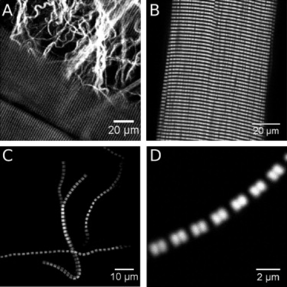
Second harmonic generation from skeletal muscle. SHG signals from muscle fibers and collagen in an entire murine extensor digitorum longus muscle (A and B), and from isolated myofibrils (C and D). The signals originate from the myosin filaments. The dip in signal intensity is located at the M-lines.

SHG polarization dependency

The SHG signal intensity changes when the plane of laser polarization is rotated (see Fig. 2). The overall minimum signal intensity is found when the electric field vector of the laser beam is orientated in parallel to the myofibril axis (α-ϕ = 0°). At angles of ∼50° and ∼130° between the electric field vector and the fibril axis the intensity is maximal, and at 90° we find a local minimum.

Figure 2.

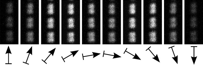
SHG orientation dependency in myofibrils. The SHG signal intensity depends on the angle of laser polarization relative to the myofibrillar axis. The minimum intensity is observed at α-ϕ = 0°, and the maximum intensities at ∼50° and ∼130° with a local minimum at 90°.

The dependency of the SHG signal intensity on the laser polarization can be concisely described with Eq. 6 or Eq. 13, as can be seen in Fig. 3. Here, two typical polarization curves are shown for myofibrils in rigor and relaxing solution, respectively. The data values are the average intensities in the ROI with the background subtracted as described above.

Figure 3.

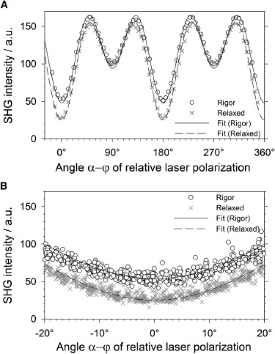
SHG laser polarization dependency. Myofibrils in relaxing and rigor solution show a different dependency on the angle of laser polarization relative to the myofibril axis. (A) The measured intensities of one rigor sample and one relaxed sample were normalized to a value of 100 for polarization perpendicular to the myofibril axis. (B) Data points from all samples, normalized as in panel A, shown in detail at the minimum intensity at α = 0°. The difference between the data sets for rigor and relaxed condition is clearly pronounced.

To illustrate the difference for rigor and relaxing solution with the sample shown in Fig. 3, we have scaled all datasets so that the data point, where the laser polarization was perpendicular to the fibril axis, has a value of 100. This normalization process does not affect the α-ϕ dependency of the curves, because for α-ϕ = 90° the SHG intensity only depends on B. This factor contains all experimental and instrumentation scaling factors. The absolute value of B is irrelevant, as we are free to set B to any value without touching the α-ϕ or γ dependency characteristics of the SHG signal.

The fitting curves shown in Fig. 3 were obtained by a nonlinear least-squares fit that used Eq. 6 as model function. One can see that the fitting curve matches the data points in good agreement (R² > 0.9, on average even R² > 0.95). Standard errors of the fitting parameters were as small as 0.1% on average.

The difference between the data sets for rigor and relaxed condition is most pronounced in the range of the minimum intensity with larger intensities in rigor solution than in relaxing solution. This difference is reflected in significantly different values for the fitting parameter γ.

Different γ-values in rigor and relaxed state

To validate the observed difference, we recorded 55 image series in total. The SHG intensity was measured in 55 ROIs with myofibrils suspended in rigor solution and in 70 ROIs with myofibrils in the relaxing solution. These data were fitted both with the simple and extended driving field model; the results are presented in Fig. 4.

Figure 4.

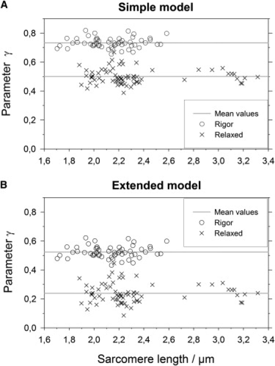
Distributions of parameter γ. (A) Simple model: There are two distinct distributions of the fitting parameter γ for the rigor state (mean 0.73, SD = 0.04, n = 55) and for the relaxed state (mean 0.50, SD = 0.05, n = 70). The parameter γ appears to be independent of the passively settled sarcomere lengths. (B) Extended model: parameter γ for the rigor state (mean 0.52, SD = 0.04, n = 55) and for the relaxed state (mean 0.24, SD = 0.07, n = 70).

One can clearly see two separate distributions of γ. In the simple model the mean values are γ_rig = 0.733 ± 0.005 (mean ± SE, n = 55) for the rigor state and γ_rel = 0.501 ± 0.006 (mean ± SE, n = 70) for the relaxed state. The same data fitted in the extended driving field model yield γ_rig = 0.524 ± 0.006 for the rigor state and γ_rel = 0.239 ± 0.008. It is interesting to note that γ does not depend on the passively settled sarcomere length of the myofibrils.

“Rigor” and “relaxed” are two extreme states with the large majority of cross-bridges attached (rigor) or detached (relaxed). To investigate whether the value change of γ is due to the binding of myosin to actin, or, alternatively, to other conformation changes, we have used an activating solution containing Ca²⁺ and the myosin inhibitor BTS (26). This combination allows myosin to bind to actin, but prevents the actual power stroke.

The mean value for n = 9 myofibrils in activating+BTS solution was γ_BTS = 0.492 ± 0.017 for the simple driving field model and γ_BTS = 0.225 ± 0.023 for the extended driving field model. A minimal decrease of γ from relaxed to activated could be observed, but the difference is not significant.

Discussion

Polarization-dependent SHG imaging probes different motor protein states

It is a well-established fact that the SHG signal from muscle preparation has its source in the myosin thick filaments (3–5,27). Myosin molecules are also responsible for muscle contraction and thus continuously change their conformation. It is therefore straightforward to hypothesize that the cross-bridge states affect the SH signal generation in the muscle.

The polarization dependence of SHG is indeed significantly different for myofibrils in either the relaxed or in the rigor state. This key result of our study is presented in Fig. 4, where two clearly separate distributions of the fitting results for the parameter γ can be distinguished. This result means that it is possible to probe different recruited or concerted steady states of the motor protein interaction with intrinsic SHG signals on a conventional two-photon microscope.

The question whether the SHG polarization dependence is affected by the myosin state has so far been addressed in two previous studies (5,28). While this article was under review, Nucciotti et al. (29) published a complementary study on state-dependent SHG signals in whole muscle fibers. A discussion of their results is included below.

For a scallop myofibril preparation, Plotnikov et al. (5) observed only a small difference between rigor and a state triggered with AMPPNP, a nonhydrolyzable ATP analog. They concluded that their measurement does not provide evidence for a significant difference. This might be due to a low sample number and a low number of recorded images per series, so that these previous results do not oppose our findings.

Nucciotti et al. have carried out polarization-dependent measurements on a whole muscle fiber preparations from rabbit (29) and frog (Rana esculenta) (28,29). In principle, their results are similar to ours, though a direct comparison of γ-values is not possible due to differences in the optical setup; see below. With a model function equal to our simple model, they obtain ${\gamma }_{\text{rig}}=0.68\pm 0.01\left(\text{mean}\pm \text{SD}\right)\text{and}{\gamma }_{\text{rel}}=0.46\pm 0.03$ for demembranated rabbit psoas fibers in the rigor and relaxed state. For single isolated fibers from frog, they report γ_rest = 0.30 ± 0.03 at rest and γ_act = 0.64 ± 0.02 at isometric tetanic contraction (29), and γ_rest = 0.273 ± 0.003 and γ_act = 0.583 ± 0.003, respectively (28). Like our finding, γ_rig is larger than γ_rel. The value for γ_act is intermediate between rigor and relaxed state; this would be expected for active cross-bridges cycling between those extreme conformations. The value for γ_rest, however, is significantly lower than γ_rel. As they point out, this might be due to structural differences of detached cross-bridges in these two conditions.

In general, we found that three factors were crucial for data acquisition and analysis of our polarization dependence recordings.

First, the optical setup must ensure a linear polarization of the laser beam at the back aperture of the objective. The half-wave plate to rotate the plane of polarization should be chosen to produce minimum elliptic polarization components at the excitation wavelength.

Second, a sufficient number of images must be recorded in each series to provide enough data points to obtain stable results from the fitting routine, especially in the minima and maxima of the polarization-dependence curve.

Third, a fair number of measurements helped us to observe the significant difference between the myosin states.

Precise γ-measurement with the extended driving field model

For a quantitatively reliable measurement of γ under high NA focus conditions, it is important to consider the effects of perpendicular and axial field components of the electric driving field. For this reason, we developed a numerical approach to extend the simple scalar model of the focus field in all three dimensions, and numerically derived a set of parameters (η_f,g, see above) with values that are specific to a certain optical setup. These parameters are then used in a more generalized model function for the polarization-dependent SHG intensity I_SHG(α-ϕ) and a value for γ can be fitted from the same raw data. It should be noted that this extension does not touch the general assumption that χ⁽²⁾ is homogeneous across the sample, or that a sample-averaged tensor is probed.

The application of this model has a large impact on the γ-values. First, the extended model γ-values are significantly lower than their simple model counterparts (see Results). Second, the difference between both populations is slightly increased. We are certain that the γ-values obtained through the extended model are closer to the real physical values. Despite this improvement we note, however, that it still relies on a theoretical model of the focus field.

Another major advantage of this approach is the introduction of comparability between different optical systems because it renders the measured results for γ independent of parameters like the imaging NA or the laser beam diameter, where the difference between simple and extended model is more pronounced for high NA lenses.

Among potential explanations for the observed differences are conformational changes of the cross-bridge and changes in the helical structure of the myosin filament: In a discussion of the molecular origin of SHG in muscle, a model was suggested (5) that associates γ via tan²θ = 2/γ with the average angle θ of single scatterers relative to the symmetry axis. Assuming single dipoles aligned on the slope of a helix, θ would be the helical pitch angle—an assumption that fits well for the collagen-I triple helix (compare θ ∼ 50° from polarization recordings (5) to 44.7° calculated from x-ray diffraction measurements (30)). For myosin with its coiled-coil of two α-helices and a pitch angle of 68.6°, previous polarization recordings yielded angles of θ = 61.2° and θ = 67.2° (5,12).

From our γ-values (extended model), we obtain 70.9° for the relaxed condition and 62.9° for the rigor condition. However, such a change in the helical pitch angle from relaxed to rigor does not seem very probable: If we assume that the arc length of the helix is constant, a change of the helix pitch from p₁ to p₂ alters the pitch angle from θ₁ to θ₂, where $\cos {\theta }_2/\cos {\theta }_1=p_2/p_1\text{∼}0.39,$ i.e., a change of ∼58 nm for a myosin molecule ∼150 nm in length (31). As the helix is very stiff along the main axis (60–80 pN/nm) (32), forces in the nanoNewton range would be necessary. This force is 2–3 orders-of-magnitude larger than the force usually developed by a single cross-bridge (33,34).

The rotating rod model can explain different γ-values

Based on our data and the reasoning above, it is most likely that the γ-value is affected by the state of the myosin cross-bridge ensemble. This is interesting because the conformation change between rigor and relaxed state takes place in the myosin head (35), whereas the major source of SHG in skeletal muscle is believed to be the light meromyosin and S2 parts of the molecule (5,27), due to its very regular, directed, and filamentous structure. Potential contributions of the globular, less directed S1 unit are uncharacterized, but assumed to be significantly lower (5).

We have developed a model based on simple geometric assumptions that can easily be extended to more complex preconditions like two-headed molecules or multiple tilting angles (29). Yet, we have found that our simplistic model can satisfactorily predict changes of γ-values based on a tilt of submolecular units (see Fig. 5). As expected, the larger the tilting fraction p of the molecule, the larger the change in γ. In the case of the myosin molecule, one obvious interpretation of p would be the relative length of the lever-arm domain, which undergoes the largest conformation change from relaxed to rigor state; the lever arm is 8 nm in length (36), so p = 0.05. Such a small value for p yields only small variations of γ, insufficient to explain the observed γ_rel and γ_rig (Fig. 5 C). Larger values of p would be necessary, e.g., by assigning a larger scatterer density to the myosin neck region which seems not very likely with the overall similar helical structure in mind.

Figure 5.

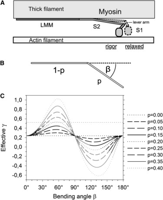
Model of cross-bridge states. (A) The myosin molecule consists of a globular head domain (S1) and a rod-shaped tail domain (S2+LMM). The free space available to tilt motions between the thick filament and the actin filament is <26 nm (see text). (B) Simplified model geometry. Fractions p of the rod-shaped molecules are bent away by an angle β from the filament axis. (C) Predicted values for γ_eff within the model parameter space. Parameter sets that are compatible with the spatial constraints in the actin-myosin lattice (see text) are depicted in black.

We tend to another applicable possibility: the tilt of the S2 domain, which is 60 nm in length. The S2 domain has a high lateral flexibility (32) and it is suspected to bend away from the filament axis as an elastic component during the power-stroke. For this case p = 0.4, or, as bends in a hinge region 44 nm from the S1 domain are frequently observed (37–39), p = 0.3. With these large values, bending or tilting can have a large effect on γ (Fig. 5). If we assume γ₀ = γ_rel, the result γ_eff = γ_rig is, in principle, covered by our model.

The potential bending angles β, however, are limited by the geometry of the actin-myosin filament lattice. The distance d₁₀ of the 1,0 lattice planes is 39.0 nm (15), which corresponds to 26 nm between the axes of an adjacent actin and myosin filament. If we also consider the size of the molecules and the filament diameters, the free space between actin and myosin is f < 20 nm. The deflection of S2 is therefore constrained by the condition $p\sin \beta <\frac{f}{l}\text{.}$

The parameter sets that meet this condition are shown in black representation in Fig. 5.

Although the parameters are in the right order of magnitude and the model predicts a correct trend for γ, it is noteworthy that no parameter set is strictly compatible with these spatial constraints. Possible reasons for these model shortcomings may include inconstant distribution of SH scatterers, residual ensemble state inhomogeneities or a break of the assumed rotational symmetry, together with azimuthal components in cross-bridge movement (40). In addition, differences in thermal jitter may play a role: In the relaxed state, thermal movements of the S1 unit are larger (40), and one can subsequently assume the same for the S2 domain. This effect would then weaken the regular spatial pattern of the cross-bridges in the relaxed state and consequently reduce the SH signal generation cross-section compared to the rigor state.

Indications for S2 domain bending during power stroke

Finally, it is of interest whether a potential bending of the myosin rod would happen while myosin binds to actin or during the actual power stroke. To investigate this question, we used high Ca²⁺/activating solution with the myosin blocker BTS. The main effect of BTS is a large decrease of the phosphate release rate (26), so that myosin molecules presumably accumulate in the prerelease A·M·ADP·P_i state. Even though this would also take effect on the equilibrium with the detached A+M·ADP·P_i state, it seems reasonable to assume that the percentage of myosin bound to actin is considerably higher here than in the relaxed state, in which actin is blocked by the troponin-tropomyosin complex (41).

If γ was related to the number of myosin molecules bound to actin per se, one would expect a considerable increase of γ_act over γ_rel. The results obtained for γ_act, however, were not significantly different from γ_rel.. This indicates that the change in γ occurs in parallel with the power stroke.

As noted above, we tend to attribute the changes of γ to a bending of the S2 domains. This assumption would then have the following consequences on S2 configuration during the cross-bridge cycle: In the rigor state, the S2 unit is bent away from the filament axis resulting in a larger γ-value. Upon myosin head detachment from actin filament, the tension on S2 is released and the observed γ-value decreases. S2 stays in this released configuration during recovery stroke and while myosin weakly binds to actin. And this is during power stroke only, when S2 is bent away from the filament axis, inducing again a larger γ = γ_rig. Notably, the steric configuration of the S1 domain itself has no significant influence on γ in this model.

Conclusions

In summary, we have shown that myofibrils in either a relaxed state or the rigor state show different polarization dependencies of SHG signals. This difference is due to differences in the χ⁽²⁾ tensor and therefore in the tensor component ratio γ. An extended model of the polarization dependence has been developed which considers the electric field distribution of high NA objectives and which allows us to extract the absolute value of γ much more precisely from measurement data. Observed differences of γ between rigor and relaxed state can be described by a simplistic geometrical model based on tilting of molecular domains, where a reasonable explanation is that the S2 domain is bent away from the filament axis during the power-stroke. The presented method and results allow us to study molecular kinetics of native myosin ensembles on a two-photon microscope.

References

- 1.Franken P.A., Hill A.E., Weinreich G. Generation of optical harmonics. Phys. Rev. Lett. 1961;7:118–119. [Google Scholar]
- 2.Roth S., Freund I. Second harmonic generation in collagen. J. Chem. Phys. 1979;70:1637–1643. [Google Scholar]
- 3.Campagnola P.J., Millard A.C., Mohler W.A. Three-dimensional high-resolution second-harmonic generation imaging of endogenous structural proteins in biological tissues. Biophys. J. 2002;82:493–508. doi: 10.1016/S0006-3495(02)75414-3. [DOI] [PMC free article] [PubMed] [Google Scholar]
- 4.Both M., Vogel M., Uttenweiler D. Second harmonic imaging of intrinsic signals in muscle fibers in situ. J. Biomed. Opt. 2004;9:882–892. doi: 10.1117/1.1783354. [DOI] [PubMed] [Google Scholar]
- 5.Plotnikov S.V., Millard A.C., Mohler W.A. Characterization of the myosin-based source for second-harmonic generation from muscle sarcomeres. Biophys. J. 2006;90:693–703. doi: 10.1529/biophysj.105.071555. [DOI] [PMC free article] [PubMed] [Google Scholar]
- 6.Llewellyn M.E., Barretto R.P.J., Schnitzer M.J. Minimally invasive high-speed imaging of sarcomere contractile dynamics in mice and humans. Nature. 2008;454:784–788. doi: 10.1038/nature07104. [DOI] [PMC free article] [PubMed] [Google Scholar]
- 7.Friedrich O., Both M., Garbe C. Microarchitecture is severely compromised but motor protein function is preserved in dystrophic MDX skeletal muscle. Biophys. J. 2010;98:606–616. doi: 10.1016/j.bpj.2009.11.005. [DOI] [PMC free article] [PubMed] [Google Scholar]
- 8.Freund I., Deutsch M., Sprecher A. Connective tissue polarity. Optical second-harmonic microscopy, crossed-beam summation, and small-angle scattering in rat-tail tendon. Biophys. J. 1986;50:693–712. doi: 10.1016/S0006-3495(86)83510-X. [DOI] [PMC free article] [PubMed] [Google Scholar]
- 9.Mertz J., Moreaux L. Second-harmonic generation by focused excitation of inhomogeneously distributed scatterers. Opt. Commun. 2001;196:325–330. [Google Scholar]
- 10.Stoller P., Kim B.-M., Da Silva L.B. Polarization-dependent optical second-harmonic imaging of a rat-tail tendon. J. Biomed. Opt. 2002;7:205–214. doi: 10.1117/1.1431967. [DOI] [PubMed] [Google Scholar]
- 11.Williams R.M., Zipfel W.R., Webb W.W. Interpreting second-harmonic generation images of collagen I fibrils. Biophys. J. 2005;88:1377–1386. doi: 10.1529/biophysj.104.047308. [DOI] [PMC free article] [PubMed] [Google Scholar]
- 12.Chu S.-W., Chen S.-Y., Sun C.K. Studies of χ2/χ3 tensors in submicron-scaled bio-tissues by polarization harmonics optical microscopy. Biophys. J. 2004;86:3914–3922. doi: 10.1529/biophysj.103.034595. [DOI] [PMC free article] [PubMed] [Google Scholar]
- 13.Berger C.L., Craik J.S., Goldman Y.E. Fluorescence polarization of skeletal muscle fibers labeled with rhodamine isomers on the myosin heavy chain. Biophys. J. 1996;71:3330–3343. doi: 10.1016/S0006-3495(96)79526-7. [DOI] [PMC free article] [PubMed] [Google Scholar]
- 14.Irving M., St Claire Allen T., Goldman Y.E. Tilting of the light-chain region of myosin during step length changes and active force generation in skeletal muscle. Nature. 1995;375:688–691. doi: 10.1038/375688a0. [DOI] [PubMed] [Google Scholar]
- 15.Millman B.M. The filament lattice of striated muscle. Physiol. Rev. 1998;78:359–391. doi: 10.1152/physrev.1998.78.2.359. [DOI] [PubMed] [Google Scholar]
- 16.Kleinman D.A. Nonlinear dielectric polarization in optical media. Phys. Rev. 1962;126:1977. [Google Scholar]
- 17.Asatryan A.A., Sheppard C.J.R., de Sterke C.M. Vector treatment of second-harmonic generation produced by tightly focused vignetted Gaussian beams. J. Opt. Soc. Am. B. 2004;21:2206–2212. [Google Scholar]
- 18.Yew E.Y.S., Sheppard C.J.R. Effects of axial field components on second harmonic generation microscopy. Opt. Express. 2006;14:1167–1174. doi: 10.1364/oe.14.001167. [DOI] [PubMed] [Google Scholar]
- 19.Yew E.Y.S., Sheppard C.J.R. Second harmonic generation polarization microscopy with tightly focused linearly and radially polarized beams. Opt. Commun. 2007;275:453–457. [Google Scholar]
- 20.Novotny L. Allowed and forbidden light in near-field optics. II. Interacting dipolar particles. J. Opt. Soc. Am. A Opt. Image Sci. Vis. 1997;14:105–113. [Google Scholar]
- 21.Cheng J.-X., Xie X.S. Green's function formulation for third-harmonic generation microscopy. J. Opt. Soc. Am. B. 2002;19:1604–1610. [Google Scholar]
- 22.Richards B., Wolf E. Electromagnetic diffraction in optical systems. II. Structure of the image field in an aplanatic system. Proc. R. Soc. Lond. A Math. Phys. Sci. 1959;253:358–379. [Google Scholar]
- 23.Leutenegger M., Rao R., Lasser T. Fast focus field calculations. Opt. Express. 2006;14:11277–11291. doi: 10.1364/oe.14.011277. [DOI] [PubMed] [Google Scholar]
- 24.Légaré F., Pfeffer C., Olsen B.R. The role of backscattering in SHG tissue imaging. Biophys. J. 2007;93:1312–1320. doi: 10.1529/biophysj.106.100586. [DOI] [PMC free article] [PubMed] [Google Scholar]
- 25.Jähne B. Oxford University Press; Oxford, UK: 1993. Spatio-Temporal Image Processing. [Google Scholar]
- 26.Shaw M.A., Ostap E.M., Goldman Y.E. Mechanism of inhibition of skeletal muscle actomyosin by n-benzyl-p-toluenesulfonamide. Biochemistry. 2003;42:6128–6135. doi: 10.1021/bi026964f. [DOI] [PubMed] [Google Scholar]
- 27.Schürmann S., Weber C., Vogel M. Myosin rods are a source of second harmonic generation signals in skeletal muscle. Proc. SPIE. 2007;6442:64421U. [Google Scholar]
- 28.Nucciotti V., Stringari C., Pavone F.S. Study of skeletal muscle cross-bridge population dynamics by second harmonic generation. Proc. SPIE. 2007;6442:644219. [Google Scholar]
- 29.Nucciotti V., Stringari C., Pavone F.S. Probing myosin structural conformation in vivo by second-harmonic generation microscopy. Proc. Natl. Acad. Sci. USA. 2010;107:7763–7768. doi: 10.1073/pnas.0914782107. [DOI] [PMC free article] [PubMed] [Google Scholar]
- 30.Beck K., Brodsky B. Supercoiled protein motifs: the collagen triple-helix and the α-helical coiled coil. J. Struct. Biol. 1998;122:17–29. doi: 10.1006/jsbi.1998.3965. [DOI] [PubMed] [Google Scholar]
- 31.Stewart M., Edwards P. Length of myosin rod and its proteolytic fragments determined by electron microscopy. FEBS Lett. 1984;168:75–78. doi: 10.1016/0014-5793(84)80209-4. [DOI] [PubMed] [Google Scholar]
- 32.Adamovic I., Mijailovich S.M., Karplus M. The elastic properties of the structurally characterized myosin II S2 subdomain: a molecular dynamics and normal mode analysis. Biophys. J. 2008;94:3779–3789. doi: 10.1529/biophysj.107.122028. [DOI] [PMC free article] [PubMed] [Google Scholar]
- 33.Finer J.T., Simmons R.M., Spudich J.A. Single myosin molecule mechanics: picoNewton forces and nanometer steps. Nature. 1994;368:113–119. doi: 10.1038/368113a0. [DOI] [PubMed] [Google Scholar]
- 34.Molloy J.E., Burns J.E., White D.C. Movement and force produced by a single myosin head. Nature. 1995;378:209–212. doi: 10.1038/378209a0. [DOI] [PubMed] [Google Scholar]
- 35.Holmes K.C. The swinging lever-arm hypothesis of muscle contraction. Curr. Biol. 1997;7:R112–R118. doi: 10.1016/s0960-9822(06)00051-0. [DOI] [PubMed] [Google Scholar]
- 36.Ruff C., Furch M., Meyhöfer E. Single-molecule tracking of myosins with genetically engineered amplifier domains. Nat. Struct. Biol. 2001;8:226–229. doi: 10.1038/84962. [DOI] [PubMed] [Google Scholar]
- 37.Walker M., Knight P., Trinick J. Properties of the myosin molecule revealed by negative staining. Micron Microsc. Acta. 1991;22:413–422. [Google Scholar]
- 38.Walker M., Knight P., Trinick J. Negative staining of myosin molecules. J. Mol. Biol. 1985;184:535–542. doi: 10.1016/0022-2836(85)90300-6. [DOI] [PubMed] [Google Scholar]
- 39.Suggs J.A., Cammarato A., Bernstein S.I. Alternative S2 hinge regions of the myosin rod differentially affect muscle function, myofibril dimensions and myosin tail length. J. Mol. Biol. 2007;367:1312–1329. doi: 10.1016/j.jmb.2007.01.045. [DOI] [PMC free article] [PubMed] [Google Scholar]
- 40.Lymn R.W. Myosin subfragment-1 attachment to actin. Expected effect on equatorial reflections. Biophys. J. 1978;21:93–98. doi: 10.1016/S0006-3495(78)85510-6. [DOI] [PMC free article] [PubMed] [Google Scholar]
- 41.Clark K.A., McElhinny A.S., Gregorio C.C. Striated muscle cytoarchitecture: an intricate web of form and function. Annu. Rev. Cell Dev. Biol. 2002;18:637–706. doi: 10.1146/annurev.cellbio.18.012502.105840. [DOI] [PubMed] [Google Scholar]