Measuring Phase-Amplitude Coupling Between Neuronal Oscillations of Different Frequencies

Abstract

Neuronal oscillations of different frequencies can interact in several ways. There has been particular interest in the modulation of the amplitude of high-frequency oscillations by the phase of low-frequency oscillations, since recent evidence suggests a functional role for this type of cross-frequency coupling (CFC). Phase-amplitude coupling has been reported in continuous electrophysiological signals obtained from the brain at both local and macroscopic levels. In the present work, we present a new measure for assessing phase-amplitude CFC. This measure is defined as an adaptation of the Kullback–Leibler distance—a function that is used to infer the distance between two distributions—and calculates how much an empirical amplitude distribution-like function over phase bins deviates from the uniform distribution. We show that a CFC measure defined this way is well suited for assessing the intensity of phase-amplitude coupling. We also review seven other CFC measures; we show that, by some performance benchmarks, our measure is especially attractive for this task. We also discuss some technical aspects related to the measure, such as the length of the epochs used for these analyses and the utility of surrogate control analyses. Finally, we apply the measure and a related CFC tool to actual hippocampal recordings obtained from freely moving rats and show, for the first time, that the CA3 and CA1 regions present different CFC characteristics.

INTRODUCTION

Neuronal oscillations of different frequencies can interact with one another (Jensen and Colgin 2007). The interaction of rhythms in different bands is commonly called “cross-frequency coupling” (CFC) and has been reported in continuous electrophysiological signals obtained at different levels, ranging from local to more mesoscopic and macroscopic scales, as assessed by intracellular, local field potential (LFP), electrocorticogram, and electroencephalogram recordings (Bragin et al. 1995; Canolty et al. 2006; Cohen 2008; Demiralp et al. 2007; Jensen and Colgin 2007; Kramer et al. 2008; Lakatos et al. 2005; Young and Eggermont 2009). In one type of interaction, known as phase-amplitude coupling or nesting, the amplitude of high-frequency oscillations is modulated by the phase of low-frequency rhythms. Perhaps the best-known example of this type of CFC occurs in the hippocampus, where the theta (5–10 Hz) phase modulates the gamma (30–100 Hz) amplitude (Bragin et al. 1995). Theoretical work suggests that such theta–gamma nesting plays a role in sequential memory organization and maintenance of working memory (Lisman 2005; Lisman and Idiart 1995).

Phase-amplitude coupling between neuronal oscillations has been receiving increasing interest, with a recent outpouring of papers in the last 5 years (Axmacher et al. 2010; Canolty et al. 2006; Cohen 2008; Cohen et al. 2009a,b; Demiralp et al. 2007; Handel and Haarmeier 2009; Hentschke et al. 2007; Jensen and Colgin 2007; Kramer et al. 2008; Lakatos et al. 2005, 2008; Schroeder and Lakatos 2009; Tort et al. 2008, 2009; Wulff et al. 2009; Young and Eggermont 2009). Phase-amplitude CFC has been reported in species such as mice (Buzsáki et al. 2003; Hentschke et al. 2007; Wulff et al. 2009), rats (Bragin et al. 1995), sheep (Nicol et al. 2009), monkeys (Lakatos et al. 2005), and humans (Axmacher et al. 2010; Canolty et al. 2006; Cohen et al. 2009a,b), and in brain regions other than the hippocampus, such as the basal ganglia (Cohen et al. 2009a; Tort et al. 2008) and the neocortex (Canolty et al. 2006; Cohen et al. 2009b; Lakatos et al. 2005). New evidence supports the idea that this type of coupling presents a functional role in the execution of cognitive functions (Axmacher et al. 2010; Cohen et al. 2009a,b; Lakatos et al. 2008; Tort et al. 2008, 2009), in accordance with theoretical models (Lisman 2005). In particular, phase-amplitude coupling has been suggested to be involved in sensory signal detection (Handel and Haarmeier 2009), attentional selection (Schroeder and Lakatos 2009), and memory processes (Axmacher et al. 2010; Tort et al. 2009).

Several methods exist for assessing phase-amplitude coupling and no single method has been chosen as the gold standard for detecting the phenomenon. The different measures possess different advantages and limitations and may be used to serve different purposes (see Cohen 2008 and present results). Here, we describe in detail a measure that we have used in recent publications for detecting phase-amplitude coupling (Tort et al. 2008, 2009). We also show how this measure compares with other measures and, based on the results, we argue that the measure we propose has properties that make it attractive for quantifying the intensity of the nesting. Finally, we present a technique related to the measure—the phase-amplitude comodulogram–which scans multiple frequency pairs searching for CFC; as an example of its application, we apply the tool to analyzing in vivo hippocampal recordings in rats performing a cognitive task and we demonstrate that the CA3 and CA1 regions may present different subbands of gamma oscillations modulated by the theta phase.

METHODS

In this section we describe how our phase-amplitude CFC measure is computed and the rationale for its definition. To be consistent with previous reports (Tort et al. 2008, 2009), we call the measure the modulation index (MI). The MI is able to detect phase-amplitude coupling between two frequency ranges of interest: the “phase-modulating” and “amplitude-modulated” frequency bands. We refer to these two frequency bands as the phase (f_p) and amplitude (f_A) frequencies, respectively. In the following text we describe the steps required for the computation of the MI.

Amplitude and phase time series extraction and the construction of the phase-amplitude plot

We denote by x_raw(t) the raw signal (e.g., the unfiltered LFP). The MI is calculated from a phase-amplitude distribution-like plot (Fig. 1), which is obtained as follows.

Fig. 1.

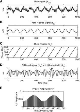
Steps in the computation of the phase-amplitude plot and modulation index (MI). The raw signal (A) is filtered at the phase (B) and amplitude (D, thin line) frequency ranges of interest. Next the phase (C) and the amplitude (D, thick line) time series are calculated from the filtered signals by using the Hilbert transform. A composite phase-amplitude time series (ϕ_fp, A_fA) is then constructed and used to obtain the mean amplitude distribution over phase bins (E; 2 cycles shown for clarity). The MI is obtained by measuring the divergence of the observed amplitude distribution from the uniform distribution. See text for further details. LG, low-gamma (30–60 Hz).

• 1) First, x_raw(t) is filtered at the two frequency ranges under analysis (f_p and f_A). We denote the filtered signals as x_fp(t) and x_fA(t).

• 2) The time series of the phases of x_fp(t) [denoted as ϕ_fp(t)] is obtained from the standard Hilbert transform of x_fp(t). The Hilbert transform is also applied to x_fA(t) to extract the time series of the amplitude envelope of x_fA(t) [denoted as A_fA(t)]. The composite time series [ϕ_fp(t), A_fA(t)] is then constructed, which gives the amplitude of the f_A oscillation at each phase of the f_p rhythm.

• 3) Next, the phases ϕ_fp(t) are binned and the mean of A_fA over each phase bin is calculated. We denote by ${\langle A_{f_A}\rangle }_{{\varphi }_{f_p}}$(j) the mean A_fA value at the phase bin j.

• 4) Last, we normalize the mean amplitude ${\langle A_{f_A}\rangle }_{{\varphi }_{f_p}}$ by dividing each bin value by the sum over the bins

  $$P(j)=\frac{{\langle A_{f_A}\rangle }_{{\varphi }_{f_p}}(j)}{{\displaystyle {\sum }_{k=1}^N{\langle A_{f_A}\rangle }_{{\varphi }_{f_p}}(k)}}$$

  where N is the number of phase bins.¹ Note then that the normalized amplitude P has the same characteristics as a discrete probability density function (pdf); that is: $P(j)\ge 0\forall j$ and ${\displaystyle {\sum }_{j=1}^{N}P(j)=1}$. Although P is not defined from a random variable—in contrast to the classical definition of a pdf—we will refer to this distribution-like function as the “amplitude distribution.” The phase-amplitude plot is obtained by plotting P as a function of the phase bin. In Fig. 1 we show this procedure outlined above for a synthetic signal using theta as f_p and low gamma (LG, 30–60 Hz) as f_A.

Note that the intensity of the phase-amplitude coupling can be already inferred by visual inspection of the phase-amplitude plot²; however, it is desirable to extract a number out of a plot like this that corresponds to the intensity of the coupling. This is what our MI measure does, as explained in the following text.

Rationale for the definition of the modulation index

Note that if there is no phase-amplitude coupling between the pair of frequencies (f_p, f_A) under study, the amplitude distribution P (defined earlier) over the phase bins is uniform, i.e., on average, the amplitude of f_A is the same for all phases of the f_p oscillation. The existence of phase-amplitude coupling is characterized by a deviation of the amplitude distribution P from the uniform distribution in a phase-amplitude plot. Following this reasoning, we defined a measure that quantifies the deviation of P from the uniform distribution. This was achieved by an adaptation of the Kullback–Leibler (KL) distance, a premetric that is widely used in statistics and in information theory to infer the amount of difference between two distributions (Kullback and Leibler 1951). The adaptation we performed was simply to make the distribution distance measure assume values between 0 and 1. Our MI is therefore a constant times the KL distance of P from the uniform distribution.

In terms of equations, the KL distance of a discrete distribution P from a distribution Q is defined as

$$D_{KL}(P,Q)={\displaystyle \sum _{j=1}^{N}P(j)\text{log}\left[\frac{P(j)}{Q(j)}\right]}$$

The KL distance has the property that D_KL(P, Q) ≥ 0 and D_KL(P, Q) = 0 if and only if P = Q, i.e., when the distributions are the same.

Notice that the KL distance formula resembles the definition of the Shannon entropy (H) of a distribution P, which is given by

$$H(P)=-{\displaystyle \sum _{j=1}^{N}P(j)\hspace{0.17em}\text{log}\hspace{0.17em}[P(j)]}$$

In fact, the KL distance is related to the Shannon entropy by the following formula

$$D_{KL}(P,\hspace{0.17em}U)=\log (N)-H(P)$$

where U is the uniform distribution. Notice further that log (N) is the maximal possible entropy value, which happens precisely for the uniform distribution [when we have P(j) = 1/N for all bins j]. Therefore because H(P) ≤ log (N), we defined our MI by dividing the KL distance of the observed amplitude distribution (P) from the uniform distribution (U) by log (N)

$$MI=\frac{D_{KL}(P,U)}{\log (N)}$$

Therefore if the mean amplitude is uniformly distributed over the phases (i.e., P = U, meaning lack of phase-amplitude coupling), we have MI = 0; MI increases the further away P gets from U, as inferred by the KL distance. An MI value of 1 happens if P is a Dirac-like distribution, that is P(k) = 1 for a given bin k and P(j) = 0 for all bins j different from k. This would denote an oscillation f_A that just exists in a single phase bin of f_p and vanishes at the other phase bins.

In Fig. 2, we show the performance of the MI in assessing different cases of phase-amplitude coupling, using theta-nested gamma as an example. Note that the MI tracks the intensity of the coupling, as seen more intuitively from the amplitude distributions.

Fig. 2.

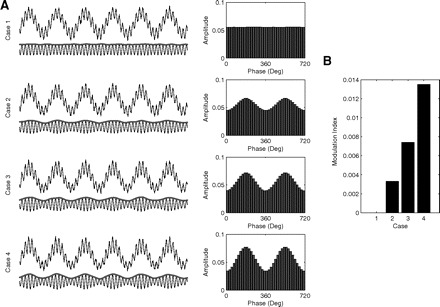
Modulation index performance in assessing phase-amplitude coupling. A, left: 4 cases differing in coupling strength are shown (top traces) along with their corresponding phase-amplitude plots (right panels). The thin and the thick traces plotted underneath show the LG filtered signal and its amplitude envelope, respectively. B: MI values for the 4 example cases shown in A.

Dependence of the MI on the data length

In this section we discuss the dependence of the MI on the length of the signal. If a given brain signal is a perfect periodic function possessing no noise component, the amount of phase-amplitude CFC can be inferred from very short epochs of the data, as long as the ϕ_fp(t) and A_fA(t) time series are longer than a full cycle of the f_p rhythm. However, given that virtually all continuous signals recorded from the brain include a significant amount of noise, a natural question that arises is how long the analyzed epoch should be to average out the noise component.

We have investigated this issue using synthetic LFPs in which we could control the length of the signal and the intensity of noise while preserving the amplitude envelope and all other parameters of the LFPs (see the appendix); this preserves what we intuitively think of as the parameters that produce the CFC. Results of this analysis are shown in Fig. 3. We ran 100 trials for each set of parameters under study (epoch length and noise intensity); we found that longer epochs led to smaller MI variation among trials, as inferred from the coefficient of variation (CV) (Fig. 3A). We also found that, in general, a higher intensity of coupling is associated with lower CV for the same epoch length (Fig. 3B). This means that strong coupling can be more confidently inferred than weak coupling for short time epochs.

Fig. 3.

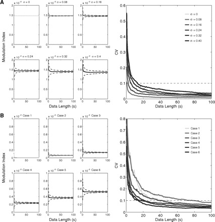
Dependence of the MI on the data length. A: plots in the left show the mean MI value as a function of the data length for 6 cases of theta–LG coupling differing in noise intensity (σ² is the variance of the white noise process; see appendix). Dashed lines denote ±SD; 100 trials were simulated for each parameter set. Notice that the mean MI approaches a steady value and that the variance among trials gets reduced with longer data lengths. The corresponding coefficient of variation (CV) levels are shown in the right plot. B: CV levels (right plot) as a function of the data length for 6 cases of theta–LG coupling differing in coupling strength (left plots). Noise level was fixed at σ = 0.24.

Note that even after defining an acceptable level for the variation in the measurements (e.g., assuming that a reliable measurement is associated with a CV of ≤10%), we are unable to recommend a universal minimal epoch length to be used in all experimental settings because the measurement is also dependent on the amount of noise present in the signal (Fig. 3A), which may vary among different data sets and laboratories. We also note that the minimal data length for a reliable measurement is dependent on the f_p frequency because slower oscillations will have fewer cycles sampled than faster oscillations. Using LFPs and studying theta as f_p, we have been typically computing the MI for epochs >30 s (i.e., >200 cycles analyzed), since we found this length long enough to provide us with a reliable measurement in our experimental setting. We recommend that each laboratory should perform its own control analysis to assess the minimal data length providing a reliable measurement (we note that this issue pertains to all CFC measures, not just the MI). In some cases, however, the nature of the paradigm used does not allow long epochs to be analyzed; to circumvent this, one can make use of surrogate control analyses to evaluate whether the measured MI can be explained by random fluctuations in the signal or whether it denotes true coupling: this is the topic of the next section.

Surrogate control analyses

When analyzing experimental results, a statistical control analysis can be performed for a single MI value to infer whether the observed value actually differs from what would be expected from chance. Common in the analysis of neurophysiological data is the generation of a chance distribution derived from the analysis of surrogate time series that shares statistical properties with the original data (Hurtado et al. 2004). To this end, the surrogate time series is usually obtained from a trial shuffling procedure, although alternative methods also exist.

In Fig. 4, we show an example of such control analysis applied to an actual theta–LG phase-amplitude plot derived from in vivo LFP recordings; these were recorded from the CA3 region of the hippocampus while a rat was performing a task. For each trial of this task, the rat is allowed to explore its current spatial context (to perform a subsequent associative choice) and the resulting phase-amplitude plot was constructed using 20 trials in a session where the animal learned the task (for details on data acquisition and task design see Tort et al. 2009). We created shuffled versions of the [ϕ_fp(t), A_fA(t)] time series by associating the phase series [ϕ_fp(t)] of trial k with the amplitude series [A_fA(t)] of trial l, with k and l randomly chosen among the trial numbers. We then generated 200 surrogate MI values, from which we could infer the MI chance distribution. As shown in Fig. 4, the trial shuffling procedure breaks the appearance of phase-amplitude coupling, which is reflected by very low MI values (mean = 1.43 × 10⁻⁵, SD = 1.12 × 10⁻⁵) compared with the measured MI value (88.29 × 10⁻⁵). Indeed, considering P < 0.01 as significant, we find that the significance threshold lies on 4.30 × 10⁻⁵, much below the experimental result. We can therefore conclude that there was real (above chance) coupling between theta-phase and LG-amplitude in CA3 while the rat was exploring the arena in our paradigm.

Fig. 4.

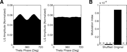
Surrogate control analysis. A: theta–LG phase-amplitude plots obtained for the original (left) and a representative trial-shuffled [ϕ_fp(t), A_fA(t)] time series (right) derived from actual hippocampal data. B: mean MI for 200 trial-shuffled and the original phase-amplitude time series. Dashed line represents the significance threshold.

As discussed earlier, the surrogate control analyses is particularly important when assessing the MI of short data epochs because random fluctuations of the signal could give rise to artifactual coupling. With long data epochs, such as the one analyzed earlier, the noise influence is less likely to affect the MI, since the noise component gets averaged out from the phase-amplitude plot when a high number of cycles is analyzed.

Comparison with other phase-amplitude coupling measures

In this section, we quickly review other phase-amplitude coupling measures and compare their performances.

1) The heights ratio

A possible CFC measure is simply to compute the ratio

$$\frac{h_{\max }-h_{\min }}{h_{\max }}$$

where h_max and h_min are the maximal and minimal amplitude heights, respectively, inferred from the same phase-amplitude plot used to compute the MI (Fig. 5A). We note that this measure has equivalent variations such as the “modulation ratio” used by Lakatos et al. (2005) defined by h_max/h_min, and also the ratio (h_max − h_min)/(h_max + h_min) used in AM radio transmission, both of which provide qualitatively similar results (not shown). We opted to use the heights ratio as defined earlier because it is intuitive and bounded between 0 and 1.

Fig. 5.

Principles underlying 3 phase-amplitude cross-frequency coupling (CFC) measures. A: the heights ratio measure can be straightforwardly defined in a phase-amplitude plot, as indicated. B: the power spectral density (PSD) of the instantaneous amplitude envelope can be used to assess phase-amplitude coupling. In this example, a theta–LG coupling measure can be defined by integrating the power values over the theta band. C: a phase-amplitude coupling measure can be defined as the length of the mean vector (arrow) of a time series defined in the complex plane by A_fAe^i∗ϕ_fp (black dots connected with line). Notice the existence of asymmetry around zero in this example, which characterizes the existence of phase-amplitude coupling in this analysis.

2) The power spectral density of the amplitude envelope

As observed by Cohen (2008), the existence of phase-amplitude modulation can be assessed by analyzing the power spectral density (PSD) of the instantaneous amplitude time series A_fA(t) (Fig. 5B). Notice that this measure has the advantage of fixing just the f_A frequency, whereas multiple f_p can be analyzed simultaneously. The occurrence of a peak in the PSD characterizes the existence of phase-amplitude coupling between f_A and the frequency band(s) where the peak(s) occurred. The CFC intensity can be inferred by the integral (or mean) power over the phase-modulating band. In the examples depicted in Figs. 1, 2, and 5, the theta–LG coupling strength is obtained by integrating the LG amplitude PSD over the theta band.

3) The mean vector length

Canolty et al. (2006) pointed out that a time series defined in the complex plane by A_fAe^i∗ϕ_fp could be used to extract a phase-amplitude coupling measure. In our example case of theta–LG coupling (Figs. 1 and 2), each instantaneous LG amplitude point is represented by the length of the complex vector [i.e., the distance from the center (0, 0)], whereas the theta phase of the time point is represented by the vector angle. In the case of an absence of phase-amplitude coupling, the plot of the A_fAe^i∗ϕ_fp time series in the complex plane is characterized by a roughly uniform circular density of vector points, symmetric around zero, because the A_fA values are on average the same for all phases ϕ_fp. If there is modulation of the f_A amplitude by the f_p phase, this means that A_fA is higher at certain phases than others. This higher amplitude for certain angles will lead to a “bump” in the complex plane plot of the A_fAe^i∗ϕ_fp time series, leading to loss of symmetry around zero. This loss of symmetry can be inferred by measuring the length of the vector obtained from the mean over all points in the complex plane. It is thus assumed that a symmetric distribution as it occurs during lack of coupling leads to a small mean vector length (because the points in the different phases would cancel each other), whereas the existence of coupling leads to a larger mean vector length (as the points in the “bump” would prevail over the others; see Fig. 5C).

4) The phase-locking value

Penny et al. (2008) and Cohen (2008) recently described new phase-amplitude CFC measures. One of these proposed measures has been named the phase-locking value (PLV) and is defined by PLV = ‖〈exp[i(ϕ_fp − ϕ_AfA)]〉‖, where ϕ_AfA is the phase time series of the amplitude envelope (see Fig. 6), 〈 · 〉 denotes the mean over all time points, and ‖ · ‖ calculates the length of the mean vector. By its definition, this measure provides the value of 1 whenever the phase series are locked and 0 if they are completely desynchronized (for a sufficiently large number of time points) and it constitutes a useful measure for detecting phase-amplitude coupling.

Fig. 6.

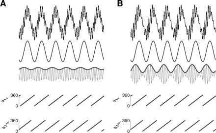
Assessing the phase-locking between the amplitude envelope A_fA and f_p. A, top panels: shown are a synthetic local field potential (LFP) example, along with the signal filtered at theta and gamma ranges bottom traces. The amplitude envelope (A_fA) of the gamma filtered signal is also shown (thick line). Bottom panels: phase time series of theta (top) and gamma amplitude (bottom). B: same as before but for a case with stronger phase-amplitude coupling (as judged by the amplitude envelope). Notice that the phase-time series of the amplitude envelope is identical to the previous case and thus the levels of phase-locking to the f_p rhythm are the same. Therefore CFC measures dependent on the level of phase-locking between A_fA and f_p are, in principle, potentially not able to track CFC intensity (for better clarity of the proof of principle, no noise was added to the synthetic signals shown in this figure).

5) The correlation coefficient

Another measure reviewed by Penny et al. (2008) is based on the assessment of the correlation between A_fA and f_p [or its normalization, defined by cos (ϕ_fp)]

$$r_{\mathit{\text{ESC}}}=\text{Corr}(f_p,A_{f_A})$$

where ESC stands for envelope-to-signal correlation. In Fig. 7 we show some examples of scatterplots between f_p and A_fA.

Fig. 7.

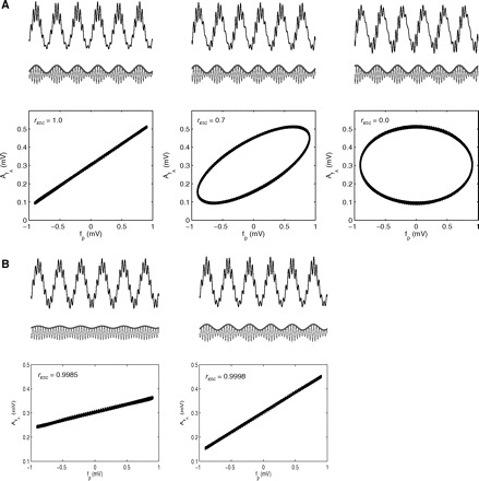
Assessing the linear regression between the amplitude envelope A_fA and f_p. A, top panels: 3 cases of phase-amplitude coupling presenting the same intensity (as judged by the amplitude envelope) but different coupling phases (top trace: synthetic LFP; bottom traces: gamma filtered signal (thin line) and gamma amplitude envelope (thick line)). Bottom panels: scatterplots between f_p and A_fA, which show that the correlation coefficient (r_ESC) depends on the phase lag between A_fA and f_p. B: 2 cases differing in CFC strength. Notice that the correlation coefficient provides similar results, since it does not depend on the slope of the regression nor on its y-intercept. Therefore CFC measures dependent on the regression between A_fA and f_p do not, in principle, correlate well with its intensity (for better clarity of the proof of principle, no noise was added to the synthetic signals shown in this figure).

6) The general linear model

As observed by Penny et al. (2008), the correlation coefficient measure described earlier has the deficiency of being influenced by the phase of the coupling. In particular, as shown in Fig. 7A, notice that this measure is not able to detect coupling at π/2 phase-difference between the f_p and A_fA. To circumvent this, Penny et al. (2008) created a new measure based on a general linear model (GLM); this measure is basically a generalization of the correlation coefficient measure that is able to detect phase-amplitude coupling at all phase lags (for details see Penny et al. 2008).

7) The coherence value

More recently, Colgin et al. (2009) used a phase-amplitude CFC tool based on the coherence spectrum between A_fA and the original signal x_raw(t). This method is based on the same principle as the PLV measure, although it uses a different tool for assessing the level of phase-locking. As in the case of the amplitude PSD, a coupling measure can be defined by integrating the coherence levels over the phase-modulating band (Colgin et al. 2009).

RESULTS

Performance comparison

Recent reports have suggested that the intensity of the phase-amplitude coupling may change depending on cognitive demands (Tort et al. 2008) and performance (Tort et al. 2009); it is thus desirable to have a metric that is able to assess the magnitude of the coupling (cf. Fig. 2), in addition to detecting its existence. As we will show in the following text, the principles underlying four of the CFC measures reviewed earlier make them potentially not suitable for measuring CFC intensity, although these measures may present a positive correlation with coupling strength in a realistic scenario where noise is present in the system.

Accordingly, the measures that are potentially not suitable to properly track the intensity of the coupling are the last four reviewed earlier: the two measures based on the levels of phase-locking between A_fA and f_p (the PLV and the coherence value) and the two measures based on the linear regression between A_fA and f_p (the correlation coefficient and the GLM). The explanation for the first case is the following: notice that different levels of phase-amplitude coupling can occur for the same level of phase-locking; the ϕ_AfA time series will be exactly the same, irrespective of the magnitude of the variation in the levels of the amplitude envelope A_fA if the level of phase locking is the same. For instance, if A_fA varies (phase-locked to f_p) between its maximal value and 90% of its maximal value or between the maximal value and 50% of its maximal value, the ϕ_AfA series will be similar in both cases, varying from 0 to 360° (see Fig. 6). Therefore in principle, neither the PLV nor the coherence value—which depend essentially on phase-locking—can properly distinguish different levels of phase-amplitude coupling.

The two measures based on linear regressions are also potentially not suitable to assess different levels of coupling because the linear correlation between two variables X and Y is the same as between X and C ∗ Y + D, where C and D are multiplicative and additive constants, respectively; notice that D corresponds to a fixed fraction of the amplitude envelope that does not vary and that different levels of coupling are reflected by different D values and regression slopes (C), which do not change the correlation/regression coefficient (see Fig. 7B).

In Fig. 8 we show the results obtained for the eight measures during the analysis of similar phase-amplitude coupling cases as in Fig. 2. For the same cases of coupling strength (as seen from the distributions shown in Fig. 8A), we have analyzed the performance of the measures under two situations differing on the presence or not of noise in the synthetic LFP. In a situation without noise (Fig. 8B), we confirmed the earlier claims that none of the measures based on the assessment of linear regression or coherence between A_fA and f_p correlates well with the CFC intensity (Fig. 8B, top row). On the other hand, all the other measures (i.e., the heights ratio, the mean vector length, and the amplitude PSD) were able to correlate with the magnitude of the CFC, similarly to the MI (Fig. 8B, bottom row).

Fig. 8.

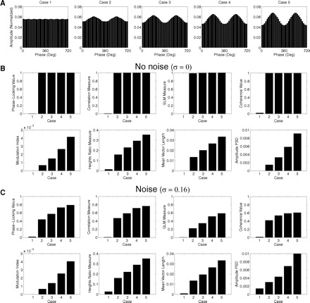
Performance comparison among 8 phase-amplitude coupling measures. A: 5 cases differing in coupling strength were analyzed. B: CFC measures values for the 5 cases shown in A in the absence of noise. Notice that the phase-locking index, the correlation measure, the general linear model (GLM) measure, and the coherence value are all able to detect phase-amplitude coupling, but do not distinguish well between different levels of coupling strength. C: similar to the above, but in the presence of noise. All measures are then able to track coupling intensity.

When analyzing synthetic LFPs with noise (the amplitude distributions of these cases are similar to Fig. 8A, since the noise gets averaged out), we then obtained that all measures, including the regression- and coherence-based measures, were able to track the intensity of the coupling (Fig. 8C). That is, although in principle four measures would not be able to correlate with CFC intensity, they end by doing so in a more noisy, realistic scenario. The reason for this is that higher levels of CFC intensity usually present a higher signal-to-noise ratio, being more easily identified than weaker cases of CFC. This is translated into a better linear regression/coherence between A_fA and f_p, explaining why the four measures discussed earlier are able to track coupling strength in the presence of noise despite the limitations intrinsic to their definition (Figs. 6 and 7).

To explore this matter further, we have assessed the tolerance of the CFC measures to random fluctuations by increasing the white noise level of our synthetic signal. The results of this analysis are shown in Fig. 9. As expected, we found that all regression- and coherence-based measures are very sensitive to noise and the values they provide present a clear negative dependence on noise level (Fig. 9, top row). We also found that all the other measures but the amplitude PSD present a good tolerance to noise (Fig. 9, bottom row).

Fig. 9.

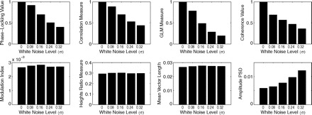
Influence of noise level on the coupling measures.

We next increased the amplitude of the LG oscillation in our synthetic LFP, while maintaining the level of coupling, and we verified that the mean vector length and the amplitude PSD measures are dependent on the absolute amplitude level of the amplitude-modulated band (Fig. 10; see also Fig. 11 for an intuitive explanation of this dependence). Although the regression- and coherence-based measures are insensitive to different levels of absolute amplitude in a situation without noise (Fig. 10C), they do present a clear positive dependence on the absolute amplitude when noise is present in the LFP (Fig. 10D); this result is readily explained by the fact that larger amplitudes are associated with a higher signal-to-noise ratio (cf. preceding discussion). Only the MI and the heights ratio measure turned out to be completely independent on the absolute level of the amplitude-modulated band (Fig. 10).

Fig. 10.

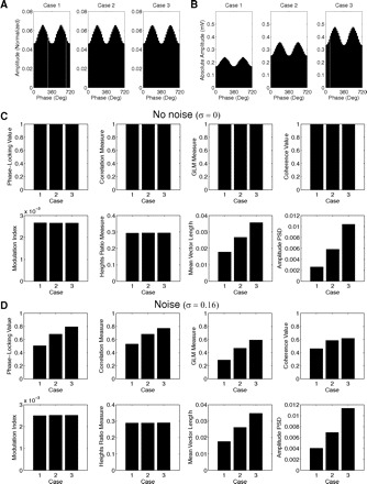
Influence of the absolute amplitude of the amplitude-modulated band on the coupling measures. A and B: 3 cases of identical coupling strength, but differing in the absolute amplitude of f_A are shown. Panels in A show the normalized amplitude (i.e., the distribution-like function P; see methods), whereas panels in B show the absolute mean amplitude level per phase bin for the same 3 cases. C: CFC measures values for the 3 cases depicted in A and B in the absence of noise. D: same as the above, but in the presence of noise.

Fig. 11.

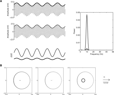
Amplitude dependence of 2 CFC measures. A, left panels: shown are 2 gamma filtered signals (top thin traces) along with their amplitude envelopes (thick traces). Notice that both examples present a similar level of phase-amplitude coupling and that the y-scale is different between both panels; the amplitude of the gamma oscillation in the second example (gray) is fivefold higher than the first (black). The bottom panel shows both amplitude envelopes plotted in the same y-scale. Right: PSD of the amplitude envelopes (same color scheme), showing that the amplitude PSD measure is dependent on the absolute amplitude. B, left 2 panels: complex plane representation of the A_fAe^i∗ϕ_fp time series obtained from the examples in A, along with their mean vector length (same color convention). Notice the different x- and y-scales. When plotted in the same scale (3rd plot from left), the different gamma amplitudes become evident. The rightmost panel shows the mean vectors for both examples plotted in the same scale. The mean vector length measure is therefore dependent on the absolute amplitude of f_A.

We also tested whether these measures would be able to detect the “width” of the modulation. As exemplified in Fig. 12A, the amplitude peak as a function of the phase can have different widths, even for the same values of maximal and minimal amplitudes. We found that the MI and the amplitude PSD seem more suitable for detecting these effects, followed by the mean vector length analysis (Fig. 12B). Clearly, the heights ratio measure is unable to detect these effects by its very definition. We also found that the regression- and coherence-based measures do not perform well in detecting the modulation width (not shown).

Fig. 12.

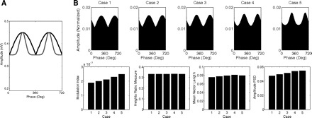
Sensitivity of the coupling measures to the “width” of the amplitude modulation by phase. A: 2 example cases plotted simultaneously (black and gray curves) illustrating that the “modulation width” can vary for the same maximal and minimal heights. B: CFC measures values (bottom) for 5 cases varying in modulation width (top).

Finally, we tested the ability of these CFC measures in detecting multimodal amplitude distributions. We note that, by their definitions, the regression- and coherence-based measures do not perform well in cases of multimodality (as also observed by Penny et al. 2008) and we have therefore focused our analysis on the other measures. As shown in Fig. 13, the heights ratio measure always assumes the same value, irrespective of the existence of multimodality, as expected from its definition. The mean vector length and the amplitude PSD measures were unable to detect symmetric multimodal distributions (Fig. 13A) (the PSD detects a coupling at twice the theta frequency in our example case). However, the latter two measures were able to detect phase-amplitude coupling in nonsymmetric cases of multimodality (Fig. 13B). On the other hand, the MI measure was able to detect both symmetric and asymmetric cases of multimodal distribution, and its values were sensitive to the different cases studied (Fig. 13).

Fig. 13.

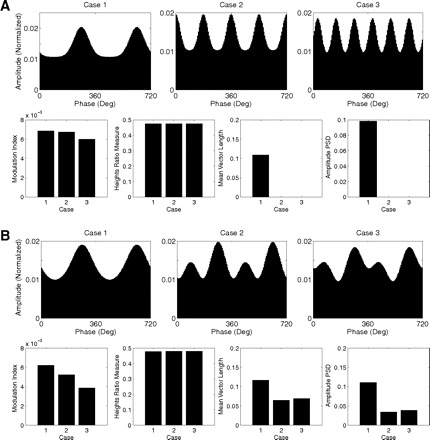
Sensitivity of the coupling measures to multimodal amplitude distributions. A and B: CFC measures values for 3 cases of symmetric (A) and asymmetric (B) multimodal amplitude distributions.

Based on the summary of these findings presented in Table 1, we conclude that the MI has some properties not shared by other measures that make it well suited for assessing the intensity of phase-amplitude coupling.

Table 1.

Summary of characteristics of the phase-amplitude coupling measures studied

Phase-Amplitude Coupling Measure	Tolerance to Noise	Amplitude Independent	Sensitivity to Multimodality	Sensitivity to Modulation Width
Modulation index	Good	Yes	Good	Good
Heights ratio	Good	Yes	No discrimination	No
Mean vector length	Good	No	Restricted	Reasonable
Amplitude PSD	Low	No	Restricted	Good
Phase-locking value	Low	No*	Restricted	Low
Correlation measure	Low	No*	Restricted	Low
GLM measure	Low	No*	Restricted	Low
Coherence value	Low	No*	Restricted	Low

^* Under the presence of noise.

Phase-amplitude comodulogram

Although the MI measure is able to examine only two frequency ranges at a time [i.e., an (f_p, f_A) pair], it can be used to construct a phase-amplitude comodulogram plot, a tool that simultaneously reports the level of coupling among multiple bands. The comodulogram is obtained by scanning frequency band pairs and applying the CFC measure to each one of them. Although computationally expensive, this analysis is ideal for searching for phase-amplitude couplings when no a priori assumptions are made about the phase-modulating (f_p) and the amplitude-modulated (f_A) frequency bands. The results are described using a pseudocolor plot that indicates the level of coupling between several narrowed-filtered frequency bands pairs. Typically, the abscissa represents the frequencies analyzed as f_p, whereas f_A is represented in the ordinate axis; that is, hot colors in a given coordinate (x, y) of the bidimensional map indicate that the phase of the x frequency modulates the amplitude of the y frequency.

In Fig. 14 we show an example of application of the comodulogram plot to actual in vivo hippocampal recordings. The comodulograms shown in this figure were constructed by using f_p calculated in 2 Hz steps with 4 Hz bandwidths and f_A in 5 Hz steps with 10 Hz bandwidths.³ The data set analyzed and the task used are the same as those used earlier (for details, see Tort et al. 2009). The comodulogram analysis was able to confirm the previously described (Bragin et al. 1995) theta-phase modulation of the amplitude of oscillations in the gamma range in the hippocampus during exploration (Fig. 14). In addition, this analysis showed that theta-phase modulated more the low-gamma (LG, 30–60 Hz) subband in the CA3 region, whereas the high-gamma (HG, 60–100 Hz) subband was more modulated in CA1 (Fig. 14). Use of a common theta-phase signal (from a fissure electrode) indicated that the peak of CA1 HG amplitude precedes the peak of CA3 LG (Fig. 14). This result therefore suggests for the first time different CFC characteristics between the CA3 and CA1 regions, while also questioning a monolithic definition for the gamma range as frequencies from 30 to 100 Hz. This example shows that new phase-amplitude CFC tools, such as the MI, and related techniques, such as the comodulogram, are able detect features about the brain rhythms that are blind to such standard tools as the Fourier analyses.

Fig. 14.

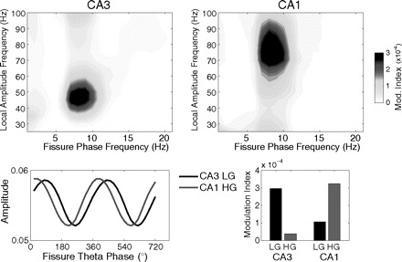
Characteristics of the gamma amplitude modulation by theta-phase differ between the CA1 and CA3 regions. Top panels: representative phase-amplitude comodulograms computed for CA3 (left) and CA1 (right) LFPs recorded simultaneously (at s. pyramidale) during context exploration. A common electrode located at the hippocampal fissure was used as the phase reference. Bottom panels: mean amplitude (normalized) per theta phase of LG in CA3 (black) and HG in CA1 (gray) for the same electrodes (left). The associated MI values are also shown (right).

DISCUSSION

We have presented a measure for assessing CFC of the phase-amplitude type. This measure (called MI) is defined as an adaptation of the KL distance, a function used to infer the distance between two distributions. Essentially, the MI is obtained by measuring the distance of an empirical amplitude distribution-like function over phase bins from the uniform distribution, which characterizes the absence of phase-amplitude coupling. We performed comparisons of the MI with other CFC measures and we showed that, by some performance benchmarks, the MI is well suited for assessing the intensity of the coupling. Finally, we have applied the MI and related techniques to actual hippocampal recordings obtained from freely moving rats; these tools were able to detect previously described theta–gamma nesting in the hippocampus and also revealed characteristics about this coupling that were not known before.

Phase-amplitude coupling among brain rhythms has been receiving increasing interest, particularly because new findings are starting to link this phenomenon to the execution of cognitive functions (see introduction). Along with the growth of interest in phase-amplitude CFC, there was a parallel development of new tools for studying these effects. In the present work, we have discussed eight tools (including ours) that were recently developed. The different tools are based on different principles and thus each tool is suited to a specific purpose. For instance, the method devised by Cohen (2008) is strong at detecting transient coupling in short time epochs. Other measures, such as the heights ratio and the amplitude PSD, possess the advantage of being straightforward, which is likely to help convince readers of the findings reported.

A main limitation of the heights ratio measure, however, is that it takes into account only the amplitude information present in two phase bins (those with the maximal and minimal heights) while discarding the mean amplitude values in the other phase bins. This measure is thus unable to detect the width of the modulation; that is, for the same maximal and minimal heights, there can be a narrow or a wide modulation around the maximal height (Fig. 12). This measure will also not distinguish unimodal from multimodal cases of phase-amplitude coupling as, for instance, in a biphasic amplitude distribution (Fig. 13).

The amplitude PSD, on the other hand, turned out to be very sensitive to noise (Fig. 9). This sensitivity is readily explained if one considers that adding white noise to a signal is equivalent to adding a constant value to its PSD. In fact, the amplitude PSD has the important caveat of depending on the absolute amplitude of f_A: for the same level of phase-amplitude coupling (as inferred by the heights ratio, for instance), the integral of the PSD will be higher for higher f_A amplitudes (Figs. 10 and 11). This caveat also hinders the comparison of CFC intensities among different bands because the different rhythms [e.g., low (30–60 Hz) and high (60–100 Hz) gamma] have different amplitudes, usually following a 1/f law. We found that normalizing and expressing the PSD as relative power (or “% Power”) makes it an inefficient phase-amplitude coupling measure for the purpose of quantifying the CFC intensity, although the normalized PSD is still able to detect the presence of coupling (not shown).

We also make two observations about the mean vector length measure: 1) a “small” or “large” mean vector length is a relative concept that depends on the f_A amplitude. For instance, during the same presence (or absence) of coupling, the mean vector length will be higher for a higher f_A amplitude (Fig. 10). In other words, like the amplitude PSD measure, the mean vector length is also dependent on the absolute amplitude of the f_A rhythm (Figs. 10 and 11). This caveat, however, can be circumvented by working with normalized mean vector length measures, as performed by Canolty et al. (2006). 2) This measure provides low values when the A_fAe^i∗ϕ_fp time series is symmetric in the complex plane, as happens during the absence of coupling. However, a bimodal distribution of amplitude modulation can also produce cases that will not be detected by this measure (e.g., if the LG amplitude has two symmetric local maximums, one at the theta phase of ϕ and another at ϕ + π, then the two amplitude “bumps” will mutually cancel each other in the mean vector analysis).

We have reviewed two measures based on linear regression and two measures based on the levels of phase-locking between A_fA and f_p (i.e., the correlation coefficient, the GLM, the PLV, and the coherence value, respectively). We showed that something curious happens with these four measures: although in principle (see Figs. 6 and 7) they should not be able to correlate with CFC intensity, they do present a positive correlation with CFC intensity in a realistic, noisy scenario. In fact, we have applied these measures to actual hippocampal LFP recordings, in which we have previously found increased theta–gamma coupling with learning (Tort et al. 2009), and we observed that these measures, similarly to the MI, were also able to track changes in CFC intensity (not shown). We concluded that differences in the signal-to-noise ratio associated with different coupling strengths likely underlie these effects. Consistent with this, we found that these measures are very sensitive to the levels of noise present in the signal (Fig. 9). Moreover, we found that these measures depend on the absolute amplitude of f_A in the presence of noise (Fig. 10); again, this dependence is likely explained by the fact that a higher f_A amplitude is associated with a higher signal-to-noise ratio. In light of these observations, we recommend care when analyzing results derived from the use of these techniques.

Recent reports have suggested that the strength of the phase-amplitude coupling may change depending on cognitive demands (Tort et al. 2008). It is therefore desirable to have a metric that correlates well with the intensity of the coupling. As we have stressed when reviewing the coupling measures, there is a difference between being able to detect the phenomenon and to correlate with its intensity. We have devised our MI as a measure that is able to both detect and quantify the intensity of the coupling. We have relied on statistics and information theory to select a function that seemed suitable for this purpose: the KL distance. Although our measure is less intuitively understood, we believe this disadvantage is compensated by its performance (Table 1).

However, it should be remarked that we have here mainly studied the ability of these CFC tools in tracking the intensity of the coupling, as intuitively inferred by the visual inspection of phase-amplitude plots; although this parameter is of interest since it has been related to cognitive functioning (Tort et al. 2008, 2009), we note that this is a particular definition of “CFC intensity,” among others possible. Depending on the research protocol, one may be more interested in tracking the coherence between the amplitude envelope A_fA and the phase-modulating rhythm f_p, irrespective of the magnitude of the variations in A_fA. In this case, both the coherence value and the PLV measures would be more appropriate measures than the MI. It should also be noted that the MI loses time information and it cannot tell us whether the coupling occurred during the whole epoch being analyzed or whether there occurred bursts of coupling inside the epoch. On the other hand, measures based on the coherence or the regression between A_fA and f_p can give us a better idea of how consistent the coupling was in the whole epoch. Similarly, other CFC measures can be better suited than the MI for assessing other particular aspects of the data; assessing the CFC intensity—as defined in this work—is just one particular feature that can be studied in these signals.

We believe that the use of these new CFC tools should give rise to significant new findings in the coming years. In the present report we have provided an example of this, by showing that the CA3 and CA1 regions can have different subbands of gamma modulated by theta phase. Previously, we also reported novel high-frequency oscillations (HFOs) in the hippocampus that were detectable only by means of CFC analyses, and we showed that the amplitude of HFO and gamma oscillations can peak at different phases of theta (Tort et al. 2008). Such CFC tools give clues to the physiological underpinnings of the dynamics and should facilitate the understanding of both the biophysical origins and the functions of brain dynamics.

Historical notes, new and classical references

References relevant to the MI measure include the classical paper by Shannon (1948) and the pioneer work by Kullback and Leibler (Kullback and Leibler 1951; see also Kullback 1959, 1987). More information on the Kullback–Leibler distance can be found in standard textbooks of statistics and information theory, as well as in science encyclopedias online.

To the best of our knowledge, the MI equation that we used was applied for the first time to neuroscience research by Tass et al. (1998). In this work, the authors applied this index to measure the divergence of phase-difference distributions from the uniform distribution. Therefore under their protocol, this measure was applied as a phase–phase coupling measure. The use of MI as a phase-locking measure has been reviewed by Le Van Quyen et al. (2001), Hurtado et al. (2004), and Young and Eggermont (2009) among others. The first application of the MI as a phase-amplitude coupling measure was done in Tort et al. (2008), in which phase–amplitude distributions were analyzed. Notice that because the MI is essentially a measure of distance from a uniform distribution, it has a wide applicability. What makes the MI specific to phase–phase coupling, or phase–amplitude coupling, or to any other effect under study, is the nature of the distribution being analyzed.

Analyses of multiple frequency pairs and expression of the results of a phase-amplitude CFC measure as a single bidimensional color map (the “comodulogram”) was previously performed in Canolty et al. (2006) and Colgin et al. (2009) for their respective coupling measures and in recent work of ours (Tort et al. 2008, 2009) for the modulation index described here.

GRANTS

This work was supported by National Institute of Mental Health Grants MH-71702 and MH-51570 to R. Komorowski and H. Eichenbaum, a National Science Foundation grant to N. Kopell, and a Conselho Nacional de Desenvolvimento Científico e Tecnológico grant to A.B.L. Tort.

DISCLOSURES

No conflicts of interest, financial or otherwise, are declared by the author(s).

APPENDIX

Our synthetic signal was modeled as⁴

$$x_{raw}(t)=A_{f_A}(t)\text{sin}(2\pi f_{A}t)+{\overline{A}}_{f_p}\text{sin}(2\pi f_{p}t)+W(t)$$

where W(t) is a Gaussian white noise process of variance σ² and Ā_fp is a constant determining the amplitude of f_p. In our simulations, the amplitude envelope A_fA(t) of the “amplitude modulated” rhythm assumed different shapes, according to the different cases studied. In the cases of unimodal distribution, the amplitude envelope was defined as

$$A_{f_A}(t)={\overline{A}}_{f_A}\frac{(1-\chi )\text{sin}(2\pi f_{p}t)+1+\chi }{2}$$

where Ā_fp is a constant that determines the maximal amplitude of f_A and χ ∈ [0, 1] is the fraction of the amplitude envelope that is not modulated by f_p; the parameter χ thus controls the intensity of the coupling (notice that χ = h_min/h_max in the phase-amplitude plot; see Fig. 5A).

For studying the width of the modulation, the amplitude envelope was modeled as follows

$$A_{f_A}(t)={\overline{A}}_{f_A}\left[(1-\chi )g(f_p,t)+\chi \right]$$

where g : ℝ⁺ × ℝ⁺ → [0, 1] is a normalized Gaussian function defined by

$$g(f_p,t)=\frac{\Phi \left[s(f_p,t)\right]-\min \left[\Phi (s)\right]}{\max \left[\Phi (s)\right]-\min \left[\Phi (s)\right]}$$

where Φ denotes a normal distribution function with zero mean and variance σ̂² and s(f_p, t) is a sawtooth wave of frequency f_p. The width of the modulation can therefore be controlled by varying σ̂².

The modeling of multimodal phase-amplitude distributions was done by using a mixture of Gaussian functions defined similarly as before, but presenting different phase lags in the sawtooth wave.

The MATLAB scripts used to compute the phase-amplitude plots and the MI can be obtained on request to the authors.

REFERENCES

- Axmacher N, Henseler MM, Jensen O, Weinreich I, Elger CE, Fell J. Cross-frequency coupling supports multi-item working memory in the human hippocampus.Proc Natl Acad Sci USA 107: 3228–3233, 2010 [DOI] [PMC free article] [PubMed] [Google Scholar]
- Bragin A, Jando G, Nadasdy Z, Hetke J, Wise K, Buzsáki G. Gamma (40–100 Hz) oscillation in the hippocampus of the behaving rat.J Neurosci 15: 47–60, 1995 [DOI] [PMC free article] [PubMed] [Google Scholar]
- Buzsáki G, Buhl DL, Harris KD, Csicsvari J, Czeh B, Morozov A. Hippocampal network patterns of activity in the mouse.Neuroscience 116: 201–211, 2003 [DOI] [PubMed] [Google Scholar]
- Canolty RT, Edwards E, Dalal SS, Soltani M, Nagarajan SS, Kirsch HE, Berger MS, Barbaro NM, Knight RT. High gamma power is phase-locked to theta oscillations in human neocortex.Science 313: 1626–1628, 2006 [DOI] [PMC free article] [PubMed] [Google Scholar]
- Cohen MX. Assessing transient cross-frequency coupling in EEG data.J Neurosci Methods 168: 494–499, 2008 [DOI] [PubMed] [Google Scholar]
- Cohen MX, Axmacher N, Lenartz D, Elger CE, Sturm V, Schlaepfer TE. Good vibrations: cross-frequency coupling in the human nucleus accumbens during reward processing.J Cogn Neurosci 21: 875–889, 2009a [DOI] [PubMed] [Google Scholar]
- Cohen MX, Elger CE, Fell J. Oscillatory activity and phase-amplitude coupling in the human medial frontal cortex during decision making.J Cogn Neurosci 21: 390–402, 2009b [DOI] [PubMed] [Google Scholar]
- Colgin LL, Denninger T, Fyhn M, Hafting T, Bonnevie T, Jensen O, Moser MB, Moser EI. Frequency of gamma oscillations routes flow of information in the hippocampus.Nature 462: 353–357, 2009 [DOI] [PubMed] [Google Scholar]
- Demiralp T, Bayraktaroglu Z, Lenz D, Junge S, Busch NA, Maess B, Ergen M, Herrmann CS. Gamma amplitudes are coupled to theta phase in human EEG during visual perception.Int J Psychophysiol 64: 24–30, 2007 [DOI] [PubMed] [Google Scholar]
- Handel B, Haarmeier T. Cross-frequency coupling of brain oscillations indicates the success in visual motion discrimination.NeuroImage 45: 1040–1046, 2009 [DOI] [PubMed] [Google Scholar]
- Hentschke H, Perkins MG, Pearce RA, Banks MI. Muscarinic blockade weakens interaction of gamma with theta rhythms in mouse hippocampus.Eur J Neurosci 26: 1642–1656, 2007 [DOI] [PubMed] [Google Scholar]
- Hurtado JM, Rubchinsky LL, Sigvardt KA. Statistical method for detection of phase-locking episodes in neural oscillations.J Neurophysiol 91: 1883–1898, 2004 [DOI] [PubMed] [Google Scholar]
- Jensen O, Colgin LL. Cross-frequency coupling between neuronal oscillations.Trends Cogn Sci 11: 267–269, 2007 [DOI] [PubMed] [Google Scholar]
- Kramer MA, Tort ABL, Kopell NJ. Sharp edge artifacts and spurious coupling in EEG frequency comodulation measures.J Neurosci Methods 170: 352–357, 2008 [DOI] [PubMed] [Google Scholar]
- Kullback S. Information Theory and Statistics. New York: Wiley, 1959 [Google Scholar]
- Kullback S. The Kullback–Leibler distance.J Am Statist Assoc 41: 340–341, 1987 [Google Scholar]
- Kullback S, Leibler R. On information and sufficiency.Ann Math Stat 22: 79–86, 1951 [Google Scholar]
- Lakatos P, Karmos G, Mehta AD, Ulbert I, Schroeder CE. Entrainment of neuronal oscillations as a mechanism of attentional selection.Science 320: 110–113, 2008 [DOI] [PubMed] [Google Scholar]
- Lakatos P, Shah AS, Knuth KH, Ulbert I, Karmos G, Schroeder CE. An oscillatory hierarchy controlling neuronal excitability and stimulus processing in the auditory cortex.J Neurophysiol 94: 1904–1911, 2005 [DOI] [PubMed] [Google Scholar]
- Le Van Quyen M, Foucher J, Lachaux J, Rodriguez E, Lutz A, Martinerie J, Varela FJ. Comparison of Hilbert transform and wavelet methods for the analysis of neuronal synchrony.J Neurosci Methods 111: 83–98, 2001 [DOI] [PubMed] [Google Scholar]
- Lisman J. The theta/gamma discrete phase code occurring during the hippocampal phase precession may be a more general brain coding scheme.Hippocampus 15: 913–922, 2005 [DOI] [PubMed] [Google Scholar]
- Lisman JE, Idiart MA. Storage of 7 ± 2 short-term memories in oscillatory subcycles.Science 267: 1512–1515, 1995 [DOI] [PubMed] [Google Scholar]
- Nicol A, Zhan Y, Fischer H, Zhang X, Feng J, Kendrick K. Learning-related alterations in theta-nested gamma oscillations in sheep inferotemporal cortex. Program No. 192.19.2009 Neuroscience Meeting Planner. Chicago, IL: Society for Neuroscience,2009. Online [Google Scholar]
- Penny WD, Duzel E, Miller KJ, Ojemann JG. Testing for nested oscillation. J Neurosci Methods 174: 50–61, 2008 [DOI] [PMC free article] [PubMed] [Google Scholar]
- Schroeder CE, Lakatos P. Low-frequency neuronal oscillations as instruments of sensory selection.Trends Neurosci 32: 9–18, 2009 [DOI] [PMC free article] [PubMed] [Google Scholar]
- Shannon C. A mathematical theory of communication.Bell Syst Tech J 27: 623–656 379–423,1948 [Google Scholar]
- Tass P, Rosenblum MG, Weule J, Kurths J, Pikovsky A, Volkmann J, Schnitzler A, Freund HJ. Detection of n : m phase locking from noisy data: application to magnetoencephalography.Phys Rev Lett 81: 3291–3294, 1998 [Google Scholar]
- Tort ABL, Komorowski R, Manns J, Kopell NJ, Eichenbaum H. Theta–gamma coupling increases during the learning of item–context associations.Proc Natl Acad Sci USA 106: 20942–20947, 2009 [DOI] [PMC free article] [PubMed] [Google Scholar]
- Tort ABL, Kramer MA, Thorn C, Gibson DJ, Kubota Y, Graybiel AM, Kopell NJ. Dynamic cross-frequency couplings of local field potential oscillations in rat striatum and hippocampus during performance of a T-maze task.Proc Natl Acad Sci USA 105: 20517–20522, 2008 [DOI] [PMC free article] [PubMed] [Google Scholar]
- Wulff P, Ponomarenko AA, Bartos M, Korotkova TM, Fuchs EC, Bahner F, Both M, Tort ABL, Kopell NJ, Wisden W, Monyer H. Hippocampal theta rhythm and its coupling with gamma oscillations require fast inhibition onto parvalbumin-positive interneurons.Proc Natl Acad Sci USA 106: 3561–3566, 2009 [DOI] [PMC free article] [PubMed] [Google Scholar]
- Young CK, Eggermont JJ. Coupling of mesoscopic brain oscillations: recent advances in analytical and theoretical perspectives.Prog Neurobiol 89: 61–78, 2009 [DOI] [PubMed] [Google Scholar]