A Parametric Empirical Bayesian framework for fMRI‐constrained MEG/EEG source reconstruction

Abstract

We describe an asymmetric approach to fMRI and MEG/EEG fusion in which fMRI data are treated as empirical priors on electromagnetic sources, such that their influence depends on the MEG/EEG data, by virtue of maximizing the model evidence. This is important if the causes of the MEG/EEG signals differ from those of the fMRI signal. Furthermore, each suprathreshold fMRI cluster is treated as a separate prior, which is important if fMRI data reflect neural activity arising at different times within the EEG/MEG data. We present methodological considerations when mapping from a 3D fMRI Statistical Parametric Map to a 2D cortical surface and thence to the covariance components used within our Parametric Empirical Bayesian framework. Our previous introduction of a canonical (inverse‐normalized) cortical mesh also allows deployment of fMRI priors that live in a template space; for example, from a group analysis of different individuals. We evaluate the ensuing scheme with MEG and EEG data recorded simultaneously from 12 participants, using the same face‐processing paradigm under which independent fMRI data were obtained. Because the fMRI priors become part of the generative model, we use the model evidence to compare (i) multiple versus single, (ii) valid versus invalid, (iii) binary versus continuous, and (iv) variance versus covariance fMRI priors. For these data, multiple, valid, binary, and variance fMRI priors proved best for a standard Minimum Norm inversion. Interestingly, however, inversion using Multiple Sparse Priors benefited little from additional fMRI priors, suggesting that they already provide a sufficiently flexible generative model. Hum Brain Mapp, 2010. © 2010 Wiley‐Liss, Inc.

INTRODUCTION

EEG/MEG and fMRI are the most widely used functional brain‐imaging techniques. Their complementary strengths, in terms of temporal and spatial resolution, are well known, which is why they are often used within the same laboratory on the same experimental paradigms. Extracranial EEG/MEG data provide a relatively direct measure of (synchronous) neuronal local field potentials (LFP) and ensuing currents with millisecond (or higher) resolution, but localizing these within the brain is an ill‐posed inverse problem [Baillet et al.,2001]. fMRI, on the other hand, normally relies on a blood oxygen level dependent (BOLD) hemodynamic signal that can be localized in the range of millimeters, but integrates over several seconds of neuronal activity. Informally, one can compare, for example, probabilistic localizations of some temporal‐ and/or frequency‐based summary of MEG/EEG data with reliable fMRI activations in the same paradigm [Brookes et al.,2005; Korvenoja et al.,1999; Mangun et al.,1998]. In general, there is reasonable agreement, although some studies have highlighted apparent discrepancies between EEG/MEG and fMRI localizations [Gonzales‐Andino et al.,2001; Stippich et al.,1998]. However, formal approaches to the integrated analysis of these different modalities remain an active area of research, and these can take different forms [Horwitz and Poeppel,2002].

A full integration, or “fusion,” would entail a single “generative” model that would explain both types of data [Aubert and Costalat,2002; Riera et al.,2006; Sotero and Trujillo‐Barreto,2008; Trujillo‐Barreto et al.,2001]. In this framework, usually Bayesian, different data types are treated symmetrically, and the priors on model parameters are not based upon the data in either modality [Daunizeau et al.,2007; cf. below]. Developing such a generative model is the ultimate goal of multimodal fusion. However, these models are complex, requiring accurate physiological models of the mapping from neuronal activity to EEG/MEG signals and to BOLD signals. Although there is empirical evidence for a close relationship between LFPs and BOLD [Logothetis et al.,2001] as well as theoretical heuristics [Kilner et al.,2005], accepted and accurate models do not yet exist. Moreover, the more complex and realistic these models, the more difficult they are to invert, particularly given the complementary spatiotemporal resolution of MEG/EEG and fMRI data.

An alternative approach is to use data from one modality as a predictor (independent variable) for the data of another modality (dependent variable). For example, one might use some summary measure of EEG/MEG power at each fMRI sample point as a regressor in a voxel‐wise, classical statistical analysis of the fMRI data, in an attempt to localize the sources of [that partition of] the EEG/MEG data {[Debener et al.,2006; Kobayashi et al.,2007; Lemieux et al.,2001; see also Martínez‐Montes et al. [2004], for a multivariate approach, and Calhoun et al. [2006], for an ICA approach}. This is the type of “asymmetric” approach that we adopt here, except that we use partitions of the fMRI data as spatial priors on the localization of the sources of the EEG/MEG data [see also Dale et al.,2000; Daunizeau et al.,2005,in press; Lin et al.,2004; Liu et al.,1998; Phillips et al.,2002]. This way, we can estimate any temporal property of the MEG/EEG sources at any location in our solution space. We see this as a pragmatic alternative to fusion of MEG/EEG and fMRI data; one in which a realistic physiological model is not needed. Yet, it uses priors (rather than predictors) in a Bayesian framework and does not enforce a direct correspondence between the MEG/EEG and fMRI sources; that is, imposes “soft” rather than “hard” constraints [Baillet and Garnero,1997]. This is important in that MEG/EEG and fMRI data are likely to have different sensitivities to certain source configurations: for example, sources deep in the brain (far from the sensors) are likely to be represented only weakly in the MEG/EEG data, whereas very transient source activity may have minimal hemodynamic correlates [see, e.g., Nunez and Silberstein,2000, for further discussion].

Our approach benefits from a recent convergence of analysis methods for MEG/EEG and fMRI toward a common Bayesian framework, specifically, a Parametric Empirical Bayesian (PEB) framework for fMRI [Friston et al.,2002], for EEG [Phillips et al.,2005], for MEG [Mattout et al.,2006], and for fusion of EEG and MEG data [Henson et al.,2009b]. The PEB framework is a special case of Variational Bayesian methods [Wipf and Nagarajan,2009], which have also been extended to spatial models of fMRI [Flandin and Penny,2007], equivalent current dipole analysis of EEG/MEG data [Kiebel et al.,2008], and dynamical network models of fMRI [Friston et al.,2003] and MEG/EEG [David et al.,2006]. In the context of distributed EEG/MEG inversion, the PEB framework entails a two‐level, linear, hierarchical model [Phillips et al.,2005]. Unlike most other inverse methods, this framework enables one to introduce multiple constraints on source locations [Mattout et al.,2006]. This is a key, because, as we have shown below, source reconstructions are improved by allowing each regional constraint, or suprathreshold “cluster”, from the fMRI data to form a separate prior, rather than entering all fMRI clusters (or even all voxels) as a single prior. With multiple fMRI priors, their relative weighting can differ, allowing the scheme to emphasize priors that are relevant, and de‐emphasize priors that are not (owing, e.g., to clusters in which the neural basis of the BOLD signal differs from that of the MEG/EEG signal, as described earlier).

Furthermore, the PEB framework furnishes an approximation to the “model evidence.” The model evidence is crucial, not only for determining the relative weighting of the priors (through implicit evidence‐maximization), but also when one wants to select between sets of priors. Indeed, we have shown previously that the model evidence can be used to adjudicate between “valid” and “invalid” sets of spatial priors via simulations on a cortical mesh [Mattout et al.,2006]. However, this model [prior] selection has not been tested on real MEG/EEG data with real fMRI priors, which calls for a method to project multiple fMRI priors onto MEG/EEG source space.

In the next section, we have outlined the theoretical considerations behind our method. This entails a brief review of the PEB approach, followed by a more detailed consideration of methods for converting a 3D statistical parametric map (SPM), based on fMRI data, to multiple covariance components that constitute the spatial priors in a source space on the cortical surface. In the Application section, we demonstrate these methods on a dataset of 12 participants who performed a face‐processing task while concurrent MEG data (from both 102 magnetometers and 204 planar gradiometers) and EEG data (from 70 electrodes) were recorded. Spatial priors were harvested from an fMRI study using the same paradigm, but a different group of participants. This illustrates a further important ingredient of our approach, namely the use of a canonical cortical mesh [Mattout et al.,2007; see below]. We conclude by discussing future extensions of our method.

THEORY

A PEB Framework

In a series of papers [Friston et al.,2006,2008; Mattout et al.,2006; Phillips et al.,2005;], we have described an empirical Bayesian approach to inverting generative models of EEG and MEG data. This is outlined in Figure 1. The generative model starts with a cortical mesh containing several thousand dipoles oriented normal to the local mesh surface (the “source space”). The matrix containing the amplitude of each of these N _p dipoles at each time point, J, contains the parameters that we wish to estimate. Given the position and orientation of the N _s sensors relative to this mesh, a N _s × N _p matrix of leadfields for each sensor, L, can be calculated in the usual way, under quasi‐static Maxwellian assumptions (we will refer to the columns of L, which map each dipole to all sensors, as “gain vectors”). By assuming zero‐mean, multivariate Gaussian distributions for the error in both the data (sensors) and the sources, a hierarchical linear model can be formulated in which the covariance of the error at the second‐level, C⁽²⁾, becomes an empirical prior on the source parameters at the first level [hence Parametric Empirical Bayes (PEB)]. The unknown covariances at sensor and source levels can be expressed as a linear combination of a number of (co)variance components at the sensor, Q ${}_{\mathbf{\text{(1)}}}^{\mathit{\text{i}}}$, and source, Q ${}_{\mathbf{\text{(2)}}}^{\mathit{\text{i}}}$, levels, weighted by hyperparameters, λ${}_{\mathit{\text{i}}}^{\text{(}\mathit{\text{j}}\text{)}}$, which are akin to the standard regularization parameters in such ill‐posed problems. These hyperparameters can be estimated using a standard Restricted Maximum Likelihood (ReML) algorithm, which, in turn, furnishes Maximal A Posteriori (MAP) estimates of the source parameters.

Figure 1.

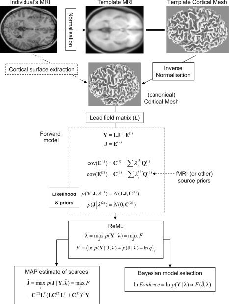
Schematic of the Parametric Empirical Bayesian (PEB) inversion scheme.

The objective function maximized by ReML, as shown in Friston et al. [2002,2007], is identical to the (negative) variational free‐energy, F. For such linear models under Gaussian assumptions, the optimized free‐energy provides a tight lower bound on the marginal log‐likelihood of the generative model, or its “log‐evidence,” , where the model is defined fully by L and Q ${}_{\mathit{\text{i}}}^{\text{(}\mathit{\text{j}}\text{)}}$. The log‐evidence increases with the accuracy of the model (e.g., fit to the data) but decreases with complexity (favoring more parsimonious models) [Penny et al.,2004]. It is this log‐evidence that we use below to evaluate the usefulness of fMRI priors, by comparing forward models in which the source covariance components, Q ${}_{\mathit{\text{i}}}^{\text{(2)}}$, reflect different combinations and types of fMRI prior.

The standard minimum norm (MNM) inversion corresponds to the simple case with one component at each of the sensor and source levels. The source‐level component is an identity matrix, that is, Q ⁽¹⁾ = I ${}_{\mathit{\text{N}}{}_{\text{s}}}$, where I _n refers to a n × n identity matrix [Phillips et al.,2005]; the sensor‐level component can be an estimate of sensor noise covariance, or, as here, another identity matrix, Q ⁽²⁾ = I ${}_{\mathit{\text{N}}{}_{\text{p}}}$, corresponding to white noise. A more recent approach is to assume multiple sparse priors (MSP), corresponding to several hundred covariance components at the source level, Q ${}_{\text{(2)}}^{\mathit{\text{i}}}$, each representing a small patch on the cortical mesh [Friston et al.,2008]. This approach has proved superior to the MNM approach, in terms of localization error and model evidence in simulations [Friston et al.,2008], and in terms of model evidence and the plausibility of source reconstructions in real data [Henson et al.,2009a]. Further mathematical details of this PEB approach are given in Appendix A.

Deriving Covariance Components from fMRI Data

In this section, we describe a generic method to derive prior covariance components (the N _p × N _p matrices Q ${}_{\mathit{\text{i}}}^{\text{(2)}}$) from a 3D volume derived from the fMRI data. This entails several steps: (1) defining a number of fMRI “clusters,” (2) projecting them onto the cortical mesh, and (3) transforming them into covariance matrices. These steps are summarized in Figure 2.

Figure 2.

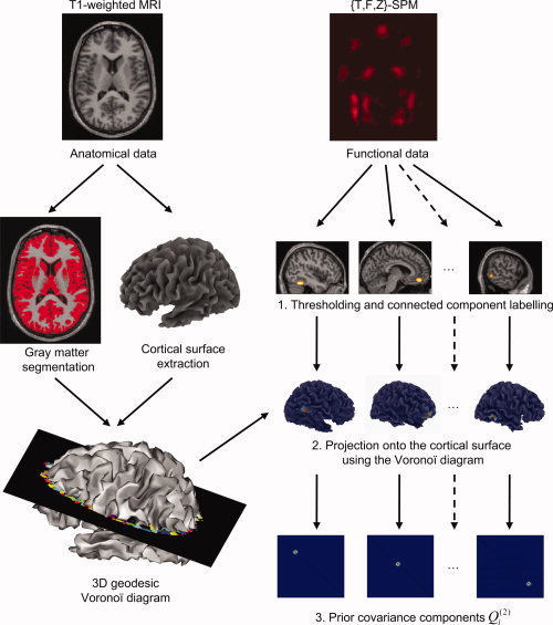
Schematic showing the derivation of prior covariance components from fMRI data used in the PEB scheme. This entails the generation of a cortical surface mesh in participant's space [this can be obtained through the inverse normalization of a canonical mesh (see Fig. 1)]. The statistical map (SPM{.}) is thresholded to form an excursion set from which clusters are formed via connected component labeling. Each cluster is then independently projected onto the surface mesh using a 3D Voronoï diagram, leading to the definition of the same number of prior covariance components.

The fMRI map, X, could contain any fMRI‐derived quantity, which has a value for each of N _v voxels within a 3D volume. In general, the number of voxels is much greater than the number of vertices, N _v ≫ N _p. Here, we consider statistical quantities such as a T‐, F‐, or Z‐statistic, which comprise a SPM. Under the null hypothesis that there is no activation (given multiple observations across scans or participants), topological features of these maps (e.g., local maxima height and cluster extent) can be assigned probabilities (P values) that quantify the risk of declaring them as “active.” Here, “active” might refer to increases in the mean BOLD response evoked by brief bursts of neural activity relative to intervening periods of baseline or by increased mean BOLD signal associated with one experimental condition relative to another. One could consider other quantities such as the mean amplitude of BOLD signal at each voxel, but given that we do not know the precise mapping between BOLD and the generators of MEG/EEG (see Introduction section), we prefer to treat our fMRI data as [probabilistic] information about location, rather than quantitative information about the magnitude of neural activity. Indeed, if one is unwilling to assume even a positive correlation between BOLD signal and whatever summary measure of MEG/EEG is being localized, one might prefer to use F‐statistics, which capture both increases and decreases in BOLD responses.

Defining the fMRI clusters

One could use the complete SPM to derive a single, continuous spatial prior on the MEG/EEG sources. However, for reasons given earlier, and vindicated in the Results section below, we define a number of discrete, spatially contiguous clusters, derived from thresholding the SPM. Below, for example, we will define clusters by the excursion set beyond a threshold calibrated to control false positive maxima to a 0.05 family‐wise level (using Random Field Theory, Worsley et al. [2005]). The clusters are then defined by connected components labeling [Haralick and Shapiro,1992] of the excursion set. One could also impose additional thresholds on the size of such clusters to remove small clusters that are unlikely to have an appreciable impact on the MEG/EEG data: The typical area of neural activity associated with detectable changes in extracranial EEG, given plausible sizes of neuronal currents, is estimated as ∼6 cm² [Nunez and Silberstein,2000]. This thresholding and labeling procedure produces images {X ⁱ}${}_{\mathit{\text{i}}\text{=1}}^{\mathit{\text{N}}\text{c}}$ corresponding to the N _c connected components or clusters that have been detected automatically. In the following, we assume that these images have been vectorized so that each X ⁱ is a vector of length N _v.

Projection of clusters onto the cortical mesh

Several methods for projecting from a 3D volume to a 2D surface have been proposed in the literature [Grova et al.,2006; Operto et al.,2008]. The crucial interpolation step can be summarized, following Kiebel et al. [2000], by:

(1)

which links the ith fMRI‐defined source to its counterpart on the cortical surface Y ⁱ, where ε_i denotes the residual error in this mapping. The function f applied to X ⁱ is the “linkage function,” whereas H is the interpolation function, defined as a N _p × N _v matrix. The choice of f and H is nontrivial. For the linkage function f, one of the simplest possibilities is the identity function f : x → x [Babiloni et al.,2001], so that the statistical values (that survived thresholding) are directly interpolated onto the mesh. Another possibility is the Heaviside function , which binarizes each fMRI prior. We compare these two choices in the Results section below. Because this comparison uses the log‐evidence, it can be regarded as optimizing the linkage function as described in Stephan et al. [2008]. In future work, it may be worth refining f such that it reflects more detailed hypotheses about the coupling between bioelectric and metabolic neural activity.

Various methods to construct the interpolation matrix H have been proposed in the literature [Andrade et al.,2001; Grova et al.,2006; Kiebel et al.,2000; Operto et al.,2008], as summarized in Appendix B. In the following, we chose a Voronoï‐based interpolation [Grova et al.,2006] for three reasons: (i) it is an anatomically informed interpolation that minimizes the interpolation errors relative to nearest neighbor or trilinear interpolation, (ii) it has a fast implementation, thanks to the use of region‐growing algorithms [Flandin et al.,2002], and (iii) it ensures that a functional cluster that overlaps with the gray matter will be overlapping as well with at least one Voronoï cell: this is especially important in our context where we want to ensure that each functional cluster provides a prior on the mesh (i.e., a cluster slightly displaced from the cortical surface will project to the cortical mesh). Note that this method requires segmentation of a (high‐resolution) structural MRI into a gray‐matter image, for which we use established methods [Ashburner and Friston,2005] and which is necessary anyway if the cortical mesh is based on that MRI.

Conversion of cortical patches to covariance components

The last step concerns creation of the covariance components or matrices necessary for the ReML source reconstruction. First, to provide yet greater robustness to misregistration errors (particularly with fMRI priors from different brains), we add a spatial smoothing step. Smoothing is achieved via a spatial coherency operator, G, which we define as the Green's function of the mesh adjacency matrix A:

(2)

where the elements of A are defined as a_ij = 1 if i and j are neighbors and 0 otherwise and σ is the smoothing parameter. Note that this smoothing uses an unweighted graph‐Laplacian and does not respect the geometry of the cortical surface (only its topology). The alternative would have been to use a weighted graph‐Laplacian [see, e.g, Chung and Taylor,2004] that incorporates the distance between vertices. In principle, the type of smoothing (and the amount of smoothing) could also be optimized by model evidence. In this work, however, we use the operator in Eq. (2), because it is computationally easier to implement (given that the adjacency matrix requires no numerical precision). We apply this operator to the cortically projected fMRI clusters, such that:

The source priors can then be formed either by creating “covariance” components via the outer product:

(3a)

or by creating a “variance” component:

(3b)

where the diag(x) operator here retains only the leading diagonal of a matrix. The difference is that a “variance” component embodies the expectation that the time courses of sources within an fMRI cluster are independent, whereas a nonzero off‐diagonal term in a “covariance” component represents the expectation that the time courses of two sources (corresponding to the row and column of that term) will be correlated (note that these matrices are not strictly covariance matrices, but rather second‐order moments, which are fit to the second‐order moment of the data, but we maintain the terms “variance”/”covariance” for ease of exposition). We explore the choice of covariance versus variance components in the Results section.

Canonical Cortical Meshes

The above procedure offers a generic method for mapping from a 3D image to a covariance component, requiring only that the 3D image (e.g., SPM) and the cortical mesh are in the same space. This alignment is simple to achieve if the fMRI data come from the same individual as the MEG/EEG data, simply by coregistering their fMRI data to their structural MRI (using standard techniques such as maximization of normalized mutual information). However, the subsequent step of extracting a consistent and highly folded tessellated mesh of the gray‐matter surface from the structural MRI is difficult to automate and requires high‐resolution, high‐contrast MR images [Mangin et al.,1995]; though we note that appropriate MR images can now be obtained quickly given recent improvements in MR scanner technologies and that this process has become fairly routine within some software, for example, [Fischl et al.,1999]. In other situations, one may prefer to use spatial constraints derived from the fMRI data from a sample of different participants. Averaging fMRI over participants normally entails warping their fMRI images to a template space, such as the Montreal Neurological Institute (MNI) space based on the coordinate system of Talairach and Tournoux [1988]. This “normalization” can be based on voxelwise matching between two MR images, constrained by priors on the typical warps required [Ashburner and Friston,2005].

Recently, we proposed a method that addresses both these issues [Mattout et al.,2007]. This method takes a template cortical mesh, which was created carefully from a typical exemplar of a set of brains within the MNI space. This mesh is then warped to match a new individual's brain, using the inverse of the warps generated when normalizing their structural MRI to the template MRI. The resulting “canonical” meshes have proved superior to using the same template mesh for all individuals, yet also sufficient, in terms of the model‐evidence, relative to cortical meshes extracted directly from individuals' MRIs, in both simulations and in the MEG data tested to date [Henson et al.,2009a; Mattout et al.,2007]. Given the importance of the orientation of sources on the gray matter surface for MEG/EEG, and the typical accuracy of spatial normalization of MR images, canonical meshes may not always allow as accurate localization as carefully created individual cortical meshes. However, there is a tradeoff between accuracy and variance, and our objective is not solely to localize accurately, but to maximize sensitivity to responses in a source space that are conserved over individuals. This is why we focus on the model‐evidence, which does not reflect accuracy per se, but rather how well the model explains the data in relation to its complexity.

The use of canonical meshes also provides a mapping between each vertex in the individual's source space and the template (MNI) space. Although one could also match cortical meshes by surface morphing techniques [e.g, Fischl et al.,1999], the use of a common template mesh (as the basis for warping to individual spaces) offers the advantage of a one‐to‐one mapping of vertices between individuals, in turn enabling methods such as the optimization of spatial priors for M/EEG over individuals [Litvak and Friston,2008]. Note also that, if one does not have access to a structural MRI of each participant (but still wishes to use spatial priors for M/EEG localization based on previous fMRI data in MNI space, e.g., from a different laboratory/study), the present framework would still permit one to use the template cortical mesh in MNI space (rather than a canonical mesh). Alternatively, if one has access to those functional MRI data, one could create a canonical cortical mesh from the warps estimated by normalizing those data to a MNI template fMRI image of the same modality.

In summary, the use of canonical cortical meshes allows the covariance components in Eq. (3) to be created directly from any SPM in MNI space (e.g., from a group analysis of different participants), using Voronoï‐based cells from a template gray‐matter partition. The individual differences associated with different locations and orientations of the dipoles associated with those vertices are then captured by the generation of the individual lead‐field matrices based on the individual canonical (inverse‐normalized) meshes.

SUMMARY

In the context of the PEB framework for the MEG/EEG inverse problem (see Fig. 1), we have described a procedure for generating the prior covariance components on 2D MEG/EEG sources from 3D fMRI SPMs (see Fig. 2). Next, we test this procedure on real data, using the free‐energy approximation to the model evidence from a standard MNM inversion to compare some of the choices that are entailed: (1) a single‐global fMRI prior versus multiple local fMRI priors, (2) “valid” versus “invalid” fMRI priors, (3) continuous versus binary priors [relating to linkage function f in Eq. (1) above], and (4) covariance versus variance priors [Eq. (3) above]. Finally, we explore the usefulness of fMRI priors in conjunction with inversions using MSP rather than MNM.

APPLICATION

To test the procedure outlined earlier, we applied it to simultaneous MEG and EEG data acquired on 12 participants during an experimental paradigm in which they performed a symmetry judgment on intermixed trials of faces and scrambled faces. The MEG data were from 102 magnetometers and 204 planar gradiometers; the EEG data were from 70 electrodes. The same data were used in a previous work that explored methods for simultaneously localizing (“fusing”) the three sensor types [Henson et al.,2009b]. Here, we localize each modality separately, allowing us to evaluate the usefulness of fMRI priors for magnetometer, gradiometer, and EEG data independently and potentially providing multiple tests of our approach.

The fMRI data came from the same paradigm, but a different group of 18 participants (reported in Henson et al. [2003]). These spatial priors live in the standard MNI space, deriving from the SPM for a group analysis of normalized images of the mean BOLD impulse response to faces and scrambled faces for each participant. Because we use a canonical cortical mesh for each of the MEG + EEG participants [Mattout et al.,2007], we have a direct mapping between the fMRI group SPM and each participant's source space.

METHODS

Participants and Paradigm

Full details of the paradigm, MEG + EEG acquisition and analysis can be found in Henson et al. [2009b]. In brief, the data came from a single, 11‐min session, in which participants saw intact faces (half familiar, half unfamiliar) or phase‐scrambled versions (approximately matched for spatial power density). Participants made left‐right symmetry judgments by pressing two keys with either their left and right index finger or left and right middle finger (most reaction times were greater than one second). The first four trials were discarded, leaving 84 intact and 84 scrambled face trials.

Data Acquisition

The MEG data were collected with a VectorView system (Elekta‐Neuromag, Helsinki, Finland), containing a magnetometer and two orthogonal, planar gradiometers located at each of 102 positions within a hemispherical array situated in a light, magnetically shielded room. The position of the head, relative to the sensor array, was monitored continuously by four Head‐Position Indicator (HPI) coils attached to the scalp. The simultaneous EEG was recorded from 70 Ag‐AgCl electrodes placed within an elastic cap (EASYCAP GmbH, Herrsching‐Breitbrunn, Germany) according to the extended 10% system and using a nose electrode as the recording reference. Vertical and horizontal EOG were also recorded. All data were sampled at 1 kHz with a band‐pass filter from 0.03 to 330 Hz.

A 3D digitizer (Fastrak Polhemus, Colchester, VA) was used to record the locations of the EEG electrodes, the HPI coils, and ∼50–100 “head‐points” along the scalp, relative to three anatomical fiducials (the nasion and left and right preauricular points). MRI images for each participant were obtained using a GRAPPA 3D MPRAGE sequence (TR = 2,250 ms; TE = 2.99 ms; flip‐angle = 9°; acceleration factor = 2) on a 3T Trio (Siemens, Erlangen, Germany) with 1‐mm isotropic voxels.

MEG + EEG Preprocessing

External noise was removed from the MEG data using the temporal extension of Signal‐Space Separation [SSS; Taulu et al.,2005], as implemented with the MaxFilter 2.0 software (Elekta–Neuromag). This software was also used to identify bad channels, to compensate for movement every 200 ms and to align the MEG data from each participant to a common coordinate frame [Taulu et al.,2005].

Manual inspection identified some bad channels (numbers ranged across participants from 0 to 11 in the case of MEG and 0 to 7 in the case of EEG). These were recreated by MaxFilter in the case of MEG [Taulu et al.,2005], but rejected in the case of EEG. The EEG data were rereferenced to the average over remaining channels. After uploading to SPM5 (http://www.fil.ion.ucl.ac.uk/spm/), the continuous data were downsampled to 200 Hz (using an antialiasing filter), further low‐pass filtered to 40 Hz in both forward and reverse directions using a fifth‐order Butterworth digital filter, and epoched from −100 to 800‐ms poststimulus onset (removing the mean baseline from −100 ms to 0 ms). Epochs in which the EEG or EOG exceeded 120 μV were rejected (mean number of rejected epochs across participants and modalities was 32), leaving 70 face epochs and 66 scrambled face epochs, on average across participants. These epochs were averaged to form a single mean evoked response to faces and scrambled faces, which were then subtracted to create a single differential evoked response (ERF/ERP).

MRI Processing and Forward Modeling

Structural MRI images of each participant were segmented and spatially normalized to an MNI template brain in Talairach space using SPM5 [Ashburner and Friston,2005]. The inverse of the normalization transformation was then used to warp a cortical mesh from a template brain in MNI space to each participant's MRI space [see Mattout et al.,2007, for further details]. This template mesh was a continuous triangular tessellation of the grey/white matter interface of the neocortex (excluding cerebellum) of 8,196 vertices (4,098 per hemisphere) with a mean intervertex spacing of ∼5 mm. The normal to the surface at each vertex was calculated from an estimate of the local curvature of the surrounding triangles [Dale and Sereno,1993].

The tissue segments in the native space of each participant's MRI were used to create a binary image of the outer scalp, which was tessellated into a mesh of 2,002 vertices using SPM. The MEG and EEG data were projected onto each participant's MRI space by a rigid‐body coregistration based on minimizing the sum of squared differences between the digitized head points (and electrode positions for EEG) and this scalp mesh using the Iterative Closest Point algorithm [Zhang,1992].

Brainstorm (http://neuroimage.usc.edu/brainstorm/) was used to fit a single sphere (for MEG) or three concentric spheres (for EEG) to the scalp mesh (using the Berg and Scherg [1994], approximation). Lead fields were then calculated for a dipole at each point in the cortical mesh, oriented normal to that mesh.

Model Inversion

The data and lead fields for each modality were projected onto N _m spatial modes, based on a singular‐value decomposition (SVD) of the outer‐product of the lead‐field matrix and using a cut‐off of exp(−16) for the normalized eigenvalues (which retained over 99.9% of the variance), resulting in 60–80 modes across participants for the magnetometer data, 91–132 for the gradiometer data, and 58–65 for the EEG data. Note that the number of spatial modes for the MEG data is actually greater than the rank of the MEG data after application of SSS, which is typically 64–69 for both magnetometers and gradiometers, so that the eigenvalues of the leadfield SVD could be truncated further. However, given that the space defined by SSS is not necessarily fully encompassed by that defined by the leadfields and that other datasets (e.g, the present EEG data) may not use signal‐projection methods like SSS, we stick with the default options in SPM here (and the presence of extraneous spatial modes should not affect the present comparisons of different fMRI priors). The data for each trial (once projected onto these spatial modes) were then reduced to N _r temporal modes for frequencies between 0 and 40 Hz inclusive within a Hanning window over the epoch, using SVD with a normalized cut‐off of 1 [Friston et al.,2006; cf, the Kaiser criterion]. This produced 2–10 temporal modes across participants and modalities, which captured a minimum of 93% of the variance over all sensor‐types and participants. These data were fit using either a standard MNM prior, corresponding to an identity matrix for the prior source covariance component, or MSP, corresponding to several hundred cortical patches (see Friston et al. [2008] for more details). A single‐identity matrix was always used for the sensor‐level covariance component (i.e., white channel noise). The differential evoked response to faces versus scrambled faces was inverted separately for each modality. To summarize the localization of the M/N170, the evoked energy at each source was averaged across samples within a time window of 150–190 ms and the square‐root taken (i.e., an RMS calculated).

fMRI Acquisition and Analysis

Full details of the fMRI acquisition and analysis can be found in Henson et al. [2003]. In brief, a 2T Vision system (Siemens, Erlangen, Germany) was used to acquire 32 T2*‐weighted transverse echoplanar images (EPI) (64 × 64, 3 × 3 mm² pixels, TE = 40 ms) per volume, with blood oxygenation level dependent (BOLD) contrast. EPIs comprised 2‐mm thick axial slices taken every 3.5 mm, acquired sequentially in a descending direction. A total of 240 volumes were collected continuously with a repetition time (TR) of 2,432 ms. The first five volumes discarded to allow for equilibration effects.

Analysis of the fMRI data was performed with SPM5. After coregistering the volumes in space and aligning their slices in time, the EPI volumes were normalized to a standard EPI template based in MNI space, resampled to 3 × 3 × 3 mm³ voxels, and smoothed with an isotropic 8‐mm full‐width‐at‐half‐maximum Gaussian kernel. The time series in each voxel was high‐pass‐filtered to 1 of 120 Hz and scaled to a grand mean of 100, averaged over all voxels and volumes.

Statistical analysis was performed using the summary statistic approach to mixed effect modeling. In the first stage, neural activity was modeled by a delta function at stimulus onset and the ensuing BOLD response was modeled by convolving these with a canonical hemodynamic response function (HRF) and its temporal and dispersion partial derivatives. Parameters for the resulting regressors were estimated by ordinary least squares. Images of the parameter estimates for each voxel comprised the summary statistics for the second‐stage analyses, which treated participants as a random effect. Here, we consider only the parameter estimate for the canonical HRF [cf. Henson et al.,2003], images of which were entered into a repeated‐measures ANOVA with three conditions corresponding to familiar faces, unfamiliar faces, and scrambled faces (correcting for nonsphericity). An SPM of the F‐statistic was then created that compared the average of familiar and unfamiliar faces against scrambled faces. This SPM{F} was thresholded for regions of at least 15 contiguous voxels (a volume of ∼0.4 cm³) that survived the threshold for local maxima of P < 0.05 (FWE‐corrected across the whole brain). This produced five clusters, shown in Figure 3A.

Figure 3.

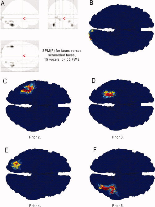
Thresholded SPM{F} for fMRI analyses in MNI space from a group of 18 participants (A), together with the patches interpolated and smoothed on the MNI template cortical mesh from. As viewed from underneath, the five fMRI clusters (B–F). Color reflects F‐value (scale irrelevant other than blue regions having value zero).

The clusters in the SPM{F} image were converted into prior spatial covariance matrices across the 8,196 dipolar sources on the cortical mesh, via the steps described earlier. This used a Voronoï interpolation based on the gray‐matter segment of the canonical MNI brain (from which the template cortical mesh was derived). Here, we used a cortical smoothness parameter of σ = 0.2 [Eq. (2)], resulting in the priors shown in Figure 3B–F; in ventral occipital and temporal lobes, with 149, 220, 139, 139, and 95 nonzero values, respectively (150 vertices would correspond to a minimal surface area of ∼7.5 cm².) We also created “invalid” priors by reflecting the original SPM{F} in the y‐ and z‐directions, resulting in five new priors, which were distributed instead over the superior aspect of the frontal lobes (141, 146, 125, 191, and 113 nonzero elements).

RESULTS

Below we explore different choices for fMRI priors, evaluating them quantitatively by T‐tests of the negative free‐energy bound on the model log‐evidence, and qualitatively in terms of the optimized hyperparameters, source reconstructions, and source time courses. We report three different analyses: (1) comparison of different sets of fMRI prior variance components (“valid,” “invalid”; local and global) under a standard MNM inversion; (2) comparison of different forms of (co)variance components (binary vs. continuous; variance vs. covariance) for (“valid,” local) fMRI priors using MNM; and (3) comparison of different sets of fMRI prior variance components when using a MSP inversion. We begin by previewing the fMRI and MEG/EEG data.

fMRI and MEG/EEG Face‐Related Responses

Regions that showed a reliable difference between faces and scrambled faces in the fMRI group analysis are shown in Figure 3A. Five clusters survived the thresholding. These are projected onto the template cortical mesh in Figure 3B–F and correspond approximately to left occipital pole, right lateral mid‐fusiform, right medial mid‐fusiform, right posterior fusiform, and left lateral mid‐fusiform, respectively. Note that these clusters represent both increases and decreases in BOLD responses evoked by faces relative to scrambled faces (indeed, the left and right lateral mid‐fusiform regions showed increased BOLD responses to faces, whereas the other three regions showed decreased responses; see also Henson et al. [2003]). Given that the precise relationship between neural activity measured by BOLD and the neural activity measured by MEG/EEG is unknown, we thought it safer to use an SPM{F}, though if one wanted to assume a positive correlation, one could use a (one‐tailed) SPM{T} instead. Note also that, because the fMRI experiment used a short, fixed Stimulus Onset Asynchrony design, it was unable to efficiently detect BOLD responses relative to the interstimulus interval of fixation [Josephs and Henson, 1999]. It is for this reason that we localized the differential evoked MEG/EEG response between faces and scrambled faces, rather than localizing the evoked MEG/EEG responses for each stimulus‐type separately, relative to the prestimulus fixation interval [cf. Henson et al.,2009b].

This differential evoked response is shown for selected sensors of each type—magnetometers, gradiometers, and EEG—by the dark line in the waveforms in Figure 4 (also shown for reference in the lighter line is the average response to faces and scrambled faces). There is little difference until around 100 ms, with a maximal difference occurring shortly before 200 ms. Indeed, these sensors were selected as those showing the greatest differential response when averaging across samples between 150 and 190 ms. This time window encompasses the M/N170 component [e.g., Bentin et al.,1996], which previous research has associated with face perception. The topographies of this mean differential response from 150 to 190 ms (which is the time‐window contrast for the source reconstructions shown later) are displayed in the lower row of Figure 4.

Figure 4.

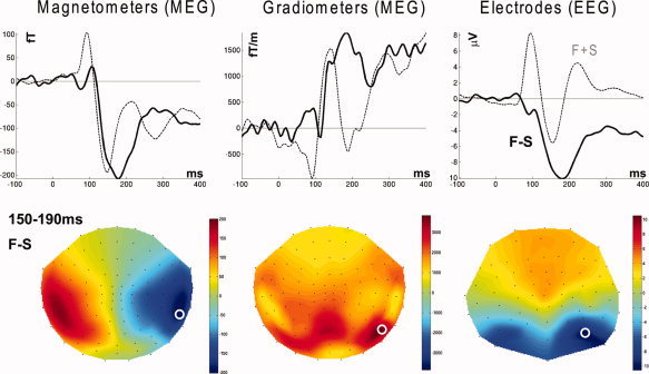
Top row: evoked waveforms from the sensor showing the maximal difference (highlighted by white circle on topographies below); dark line, differential response for face minus scrambled faces; light line, average response to faces and scrambled faces. Bottom row: sensor‐level topographies (using a spherical projection and cubic interpolation) for each type of sensor for the mean difference between faces and scrambled faces between 150 and 190 ms. Note that the magnetometer topography shows the size and direction of magnetic flux; the gradiometer topography shows the scalar magnitude (vector length) of the gradient in the two in‐plane directions; the EEG topography shows the potential difference relative to the average over all (valid) electrodes.

Analysis 1: Different Sets of fMRI Priors (Under MNM)

In this first analysis, five different models were compared using a basic MNM inversion:

Model 1.1

In the “None” (baseline) model, no fMRI priors were used, resulting in a single independent and identically distributed (IID) variance component for the sources and a single IID variance component for the sensors (i.e., N _p × N _p and N _m × N _m identity matrices respectively).

Model 1.2

In the “Global” model, the values within the i = 1…5 cortical patches, q _i, representing the smoothed, interpolated F‐statistic values from the suprathreshold fMRI clusters (see Fig. 3), were summed and binarized [Eq. (1)] to create a single‐variance component [Eq. (3b)]. This was used in addition to the IID component (which was common to all models), resulting in two source components.

Model 1.3

In the “Local (Valid)” model, the five fMRI clusters were used as separate binarized, variance components, allowing them to be “weighted” differentially via their hyperparameters to maximize the free energy.

Model 1.4

In the “Local (Invalid)” model, five different clusters over the superior frontal cortex were used as separate variance components (see Methods section).

Model 1.5

Finally, in the “Valid + Invalid” model, the five “valid” and the five “invalid” priors were used.

Effect of Global Versus No fMRI Priors

The mean negative free‐energy, F, across participants for each of the five models is shown in the columns of Figure 5; the three rows pertain to the three sensor‐types. The first interesting comparison is the effect of a single fMRI prior (“Global” Model 1.2 vs. “None” Model 1.1), which increased F reliably across participants for all sensor‐types, T(12) > 1.94, P < 0.05, one‐tailed. The effect of the global fMRI prior on the source reconstructions was mainly to pull activity slightly more medially in the posterior ventral occipitotemporal cortex (cf. first and second columns of Fig. 6), perhaps helping to counteract the well‐known bias toward diffuse superficial reconstructions associated with MNM inversions.

Figure 5.

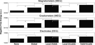
Free‐energy results for each modality and model in Analysis 1 (MNM and binary, variance components).

Figure 6.

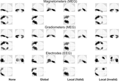
Mean conditional source reconstructions across participants for each modality and model in Analysis 1 (MNM and binary, variance components). Each panel shows a maximal intensity projection (MIP) of the 512 greatest source strengths within MNI space. For illustration purposes, the source estimates have been smoothed on the 2D mesh surface via 32 iterations of an unweighted graph Laplacian with adjacency ratio (c.f., autoregression coefficient) of 1/16.

Effect of Local Versus Global fMRI Priors

The second interesting comparison addressed the value of using separate covariance constraints for each fMRI cluster (“Local” Model 1.3 vs. “Global” Model 1.2 in Fig. 5). Despite the additional model complexity (i.e., six vs. two source priors), local priors produced a highly reliable increase in F for MEG magnetometers and gradiometers, T(12) > 4.88, P < 0.001. For EEG, there was a small numerical increase, but it was not significant, T(12) = 0.25, P = 0.81.

For the MEG data, the ability of the more complex model to weight each fMRI prior separately again resulted in a shift of activity deeper into fusiform cortex, particularly on the right (cf. second and third columns in Fig. 6). This is consistent with the relative values of the five hyperparameters: for the magnetometers and gradiometers, the hyperparameters for the right and left lateral fusiform regions were more consistently nonzero across participants than the other fMRI priors (top row of Fig. 7). For the EEG data, there was less‐consistent weighting of any one prior, most likely reflecting less information in the ∼65 channels with which to distinguish the priors (and in keeping with the nonsignificant difference in F between global and local fMRI priors for the EEG data).

Figure 7.

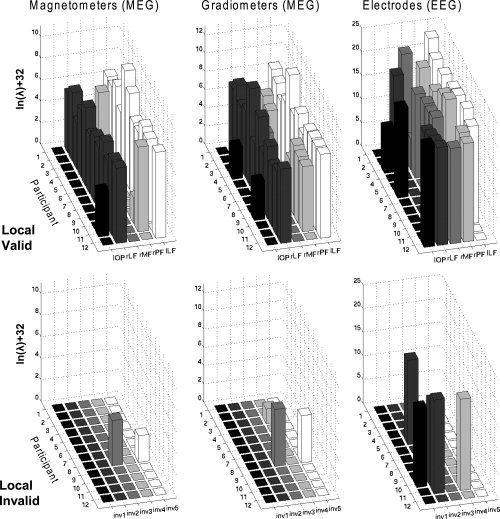
Hyperparameters for each modality and model in analysis 1 (MNM and binary, variance components). The z‐axis represents the increase in the natural log of the hyperparameters relative to their prior value (a natural log of −32) and is not comparable across sensor types (owing to different scaling and physical units).

The above results illustrate the importance of allowing a separate weighting of each fMRI prior. This makes sense if different brain regions contribute differentially to the MEG/EEG data (through different gain vectors) or if the fMRI signal in some areas, but not others, reflects neural activity that occurred outside the time window of MEG/EEG data localized. Note finally, that within the present PEB framework, sources are not constrained to have the same time courses (even within a single fMRI prior), as illustrated in Figure 8. Although the priors determine the variance of the sources, their time courses also depend on the gain vectors at each location (and the data of course). For example, the left and right lateral fusiform regions in Figure 8 show a more distinct peak between 150 and 190 ms than do the other three regions (suggesting that these regions are the primary generators of the M170; see also Henson et al. [2009b]).

Figure 8.

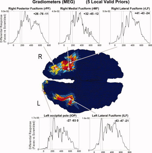
Estimated time courses from dipoles closest to maxima of each fMRI cluster within the SPM{F} (coordinates in MNI space) for five “valid” local priors in Analysis 1. Note the time course reflects the magnitude (RMS) of differential response to faces versus scrambled faces (arbitrary units; and note different scales, with significantly less activity in occipital region).

Effect of “Valid” Versus “Invalid” Local fMRI Priors

The third interesting comparison concerned the effect of using “invalid” fMRI priors (“Local Valid” Model 1.3 vs. “Local Invalid” Model 1.4 in Fig. 5). For all sensor types, “invalid” priors decreased F reliably, T(12) > 2.10, P < 0.05, one‐tailed. This empirical result reinforces the ability of our Bayesian framework to distinguish “valid” from “invalid” fMRI priors, consistent with prior simulation results [Daunizeau et al.,in press; Mattout et al.,2006; Phillips et al.,2005]. It also confirms that simply increasing the number of source priors (e.g., from one global to multiple local fMRI priors)—i.e, increasing the model complexity—does not necessarily increase F. Furthermore, the value of F for five “invalid” priors was no greater than when using no fMRI priors (“Local Invalid” Model 1.4 vs. “None” Model 1.1); indeed, there was a numerical, though not reliable, decrease for all sensor‐types, T(12) > 1.0, P < 0.34, presumably reflecting the penalty associated with greater model complexity. This result is reflected by the fact that the source reconstructions, at least for magnetometers and gradiometers, were little affected by the presence of “invalid” priors (cf. first and fourth columns in Fig. 6). This is because the hyperparameters for the “invalid” fMRI priors were mostly shrunk to zero (Fig. 7, bottom row). This discounting of “invalid” priors is encouraged by our use of shrinkage hyperpriors [Henson et al.,2007], enabling automatic relevance detection (ARD; see Appendix A).

This failure of “invalid” priors to “bias” the inverse solutions is obviously an important feature of the PEB framework [Phillips et al.,2005], particularly if the fMRI data derive from neural causes that do not generate MEG/EEG data. However, we should note that other, smaller displacements of the fMRI priors from their “valid” locations (e.g., translations of a few centimeters) often increased F relative to no fMRI priors. This presumably reflects the indeterminacy of the inverse problem, with insufficient information in the data to distinguish prior locations that entail similar gain vectors. Nonetheless, the free‐energy will always encourage “valid” priors when they are present, at the expense of “invalid” priors (through the ARD behavior). This was confirmed by the results from the final “Valid + Invalid” Model 1.5, in which both “valid” and “invalid” priors were included (i.e., 10 fMRI priors in total). As expected, F was improved relative to no priors (Model 1.1), T(12) > 1.8, P < 0.05, one‐tailed, but did not increase nor decrease reliably relative to the five “valid” priors (Model 1.3), T(12) < 0.45, P > 0.50. As expected, the source reconstructions (not shown) resembled those with the five “valid” priors only, because the hyperparameters for the “invalid” priors shrank to zero. Thus, while one should beware of adding too many fMRI priors when none is in fact “valid,” the simultaneous presence of “valid” priors is likely to overcome this problem.

Analysis 2: Nature of fMRI Covariance Components

In this second analysis, using the five “valid” fMRI priors, we compared four different models from crossing two factors: whether the covariance matrices created from the fMRI clusters corresponded to variance or covariance components (i.e., with or without off‐diagonal terms, [Eq. (3a/b)], and whether they contained the continuous or binarized versions of the fMRI F‐values [i.e., using the identity or Heaviside linkage functions in Eq. (1)]. The largest effect by far was that variance components produced higher free‐energies than covariance components, with T(12) > 2.70, P < 0.05, for all sensor‐types and binary/continuous priors, except continuous priors for EEG, which was a trend, T(12) = 1.91, P = 0.08 (see Fig. 9). For variance components, there was also evidence that binary priors produced slightly higher F than continuous priors, at least for the MEG data, T(12) > 2.37, P < 0.05 (though not reliably so for the EEG data, T(12) = 1.54, P = 0.15). For covariance components, there was no evidence that binary versus continuous made any difference, T(12) < 1.35, P > 0.21, for all three modalities. The difference between covariance and variance priors relates to whether or not the activities of dipoles within each prior covary over time. Constraining them this way may not improve the model evidence if sources within the same cluster have different time courses (e.g., if the cluster actually encompasses two functionally distinct regions). Another reason why the additional constraint may not help is if there are inaccuracies in the fMRI priors (e.g., clusters are too large): such inaccuracies are likely to be exaggerated by the additional constraint on their covariances as well as variances. Having said this, the difference in the source reconstructions and hyperparameters for variance versus covariance priors was minimal (see Supporting Information Fig. 1).

Figure 9.

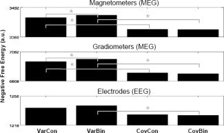
Free‐energy results for each modality and model in Analysis 2 (MNM, five local “valid” fMRI priors). Var, Variance; Cov, Covariance; Bin, Binary; Con, Continuous. Note that the second model (column) is the same as the third model (column) in Analysis 1 in Figure 5.

Analysis 3: Different Sets of fMRI Priors Using MSP

In a final set of analyses, we revisited the five models in Analysis 1 under MSP rather than MNM priors. MSP entails the use of several hundred sparse priors (756 in present data), and so one might expect little effect of adding another five fMRI priors (even if less sparse). First, MSP increased the overall negative free‐energy across all the models, relative to the equivalent MNM model, consistent with previous data ([Friston et al.,2008; Henson et al.,2009a]; cf. Figs. 10 and 5). Second, F showed little evidence of any effects of the different fMRI priors. No pairwise differences were reliable, except for magnetometers, where there was actually a reliable decrease in F when separate “valid” fMRI priors were included in the model, relative to a global prior or “invalid” priors, T(12) > 3.35, P < 0.01 [this was not true for gradiometers, T(12) < 1.39, P > 0.19, nor EEG, T(12) < 1.47, P > 0.16]. The general lack of any improvement with the addition of fMRI priors suggests that the MSP source priors are already optimal (i.e., a superset of the fMRI priors). Another possible explanation concerns the relatively “deep” sources in the anterior temporal lobe, which were predicted by MSP (see Supporting Information Fig. 2), but which were not present in the fMRI priors, and which would not be encouraged by MNM alone, given its bias toward more diffuse, superficial sources. In either case, the main result is that there is no evidence that fMRI priors improve model evidence when using MSP.

Figure 10.

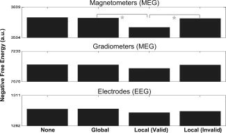
Free‐energy results for each modality and model in Analysis 3 (MSP, five local “valid” binary variance fMRI priors).

DISCUSSION

We have outlined how fMRI data can be used as spatial priors on the MEG/EEG inverse problem, within the context of an established PEB framework. This entailed a new procedure for mapping from a continuous 3D volume (e.g., a SPM based on fMRI data) to a number of matrices representing the prior covariance of source amplitudes within smooth patches on a 2D cortical sheet. Using the free‐energy bound on the model evidence, we showed how the SPM{F} from a group of 18 participant's fMRI data in MNI space could improve standard minimum‐norm inversions of MEG and EEG data from a different group of 12 participants. This improvement was greatest when each regional fMRI cluster was used as a separate spatial prior on the variance of the sources. This improvement in model evidence was accompanied by more realistic source reconstructions for the differential response to faces versus scrambled faces, in which the individual weightings (hyperparameters) for each spatial prior showed a dominance for left and right lateral fusiform sources (at least in the MEG data).

Given that the precise mapping between the causes of MEG/EEG data and causes of the fMRI (BOLD) signal is currently unknown, the Bayesian framework is well‐suited for using the fMRI data as “soft” rather than “hard” constraints. Moreover, an important novelty of our particular Bayesian approach is that we treat each suprathreshold fMRI cluster as a separate location prior. The relative influence of each prior can then be determined through the ReML maximization of the negative free‐energy. This separate weighting is also important in situations where the time window of the MEG/EEG data being localized does not include the times when the BOLD signal is generated. Further ways to minimize assumptions about the MEG/EEG‐fMRI mapping include (i) the use of F‐statistics rather than [one‐tailed] T‐statistics for the fMRI data (i.e., not assuming a positive correlation between the two types of data), (ii) the use of binary rather than continuous prior variances [i.e., using a Heaviside rather than identity function for the linkage function in Eq. (1)], and (iii) the use of variance rather than covariance priors [Eq. (3)]. Nonetheless, these are all options that can be further explored for different datasets (and evaluated quantitatively using the model evidence, as was done earlier). Other future explorations can look at (i) more sophisticated “linkage” functions, (ii) model comparisons over different peristimulus time windows, (iii) effects of the degree of mis‐location of spatial priors (effectively exploring the spatial resolution of MEG/EEG), and (iv) the effect of fMRI priors when using free rather than fixed orientation of dipoles [Henson et al.,2009a].

Further robustness in the method was achieved by using a Voronoï‐based interpolation from the 3D image to the 2D cortical surface (robust to small misregistration errors) and smoothing on the 2D surface (which ameliorates any abrupt interpolation errors). We also made use of canonical cortical meshes, which allowed us to pool fMRI data from different participants when forming priors. We expect that this will be useful for those seeking to use fMRI data to constrain MEG/EEG inversions (e.g., by using prior published fMRI results or meta‐analyses in MNI space). Nonetheless, it would also be useful to examine the value of fMRI priors when the fMRI data and MEG/EEG data are acquired on the same participants, using SPMs in their native space and individually defined cortical meshes.

The main conclusions from the MNM analyses—(i) that separate local fMRI priors are better than a global fMRI prior, (ii) that “invalid” priors (particularly in the presence of “valid” priors) can be properly discounted, and (iii) that variance components are superior to covariance components—held for MEG data from both magnetometers and gradiometers (though note that the common application of SSS during preprocessing of the MEG data means that the magnetometer and gradiometer data do not provide completely independent tests). These conclusions were also largely supported by the EEG data, though the evidence was not as strong, particularly in that the increase in model evidence for local versus global fMRI priors was not significant. This could reflect physical properties of the EEG data (e.g., its spatial smoothing by the scalp), greater errors in the leadfield matrix (given the spherical approximation used here and the sensitivity of EEG data to relative conductivities), and/or the smaller number of sensors used here (typically around 65 valid channels; cf. 102 magnetometers and 204 gradiometers). The question of whether fMRI priors are as useful for EEG as for MEG could also be explored in future studies, using more realistic forward models.

Finally, it was interesting to find that fMRI priors did not improve the model evidence when using MSP, rather than the more conventional MNM prior. This suggests that MSP priors were sufficiently flexible to subsume any additional fMRI priors (consistent with the more focal and deeper sources resulting from MSP). In theory, however, there are other source distributions (e.g., extensive and superficial activities) where MNM can have a higher model evidence than MSP, and in which fMRI priors may remain useful. Again, it will be interesting to explore this in other MEG/EEG plus fMRI datasets. Having said this, the whole point of MSP is to optimize the priors themselves. Crucially, redundant priors are “switched off” through the use of shrinkage priors and evidence maximization implicit in the ReML scheme. This means that if the fMRI priors can be expressed as a mixture of MSPs, the fMRI priors are redundant. Indeed, this is what our model comparison results suggest. If it were possible to find fMRI priors that increased the evidence for a model that included MSPs, then this would be very interesting and provide pointers to better MSPs.

It is important to remember that the present results pertain to a specific dataset, and the conclusions regarding the various choices of fMRI prior might not generalize to other datasets. Furthermore, future studies could test the generalization of the conclusions to other forward models and other inverse solutions; of particular importance would be to test the results when using more accurate forward models than the spherical‐based models used here, such as boundary‐element models. Nonetheless, the main value of this study is to outline some of the choices available for using fMRI as spatial constraints on M/EEG localization and demonstrate how those choices can be evaluated in the context of the model‐evidence within an empirical Bayesian framework.

The present “asymmetric” approach of using the data in one modality as priors on inverting another may represent a prelude to a full “symmetric” approach to multimodal fusion, in which a single generative model is inverted, as we have demonstrated for fusion of EEG and MEG data [Henson et al.,2009b]. However, there is a possibility that the hopes for multimodal fusion of fMRI and MEG/EEG may be misplaced. Unlike the fusion of MEG and EEG, the parameters of generative models for hemodynamic and electromagnetic signals may not be shared. Put simply, if all we can estimate from fMRI data is “where” signals are coming from (i.e., spatial parameters) and all we can estimate from MEG/EEG data is “when” those signals are expressed (i.e., temporal parameters), then there is no point in using a common generative model. This is because multimodal fusion provides multiple constraints on the estimation of unknown quantities generating data. If these quantities are constrained by only one modality, the conditional precision of their estimates will not be increased by adding another. The only way that fusion can work is if the spatial parameters estimated precisely by fMRI depend on the temporal parameters estimated precisely by MEG/EEG (or vice versa). Unfortunately, there is no principled reason to think that there will be strong dependencies of this sort, because the dynamics of electromagnetic sources are formally similar in different parts of the brain. If this argument turns out to be true, then the most powerful approaches may be asymmetric: that is, using MEG/EEG as temporal constraints in whole‐brain fMRI models or using fMRI as spatial priors on the EEG/MEG inverse problem, as considered here.

Software Note

The algorithms described in this work will be available in the academic software SPM8, which can be downloaded from http://www.fil.ion.ucl.ac.uk/spm/.

Supporting information

Additional Supporting Information may be found in the online version of this article.

Supporting Figure 1

Supporting Figure 2

APPENDIX A.

We assume a hierarchical linear model with Gaussian errors that can be formulated in a PEB framework [Phillips et al.,2005]. This corresponds to a two‐level model, with the first level representing the sensors and the second level representing the sources:

where Y is an N _s (sensors) ×N _t (time points) matrix of sensor data; L is a N _s × N _p (sources) matrix representing the “forward model”, and J is the N _p × N _t matrix of unknown dipole currents; that is, the model parameters that we wish to estimate. E ₁ and E ₂ represent zero‐mean, multivariate Gaussian distributions that assume a spatiotemporal factorization into temporal covariance, V, and spatial covariances C ⁽¹⁾ and C ⁽²⁾ [Friston et al.,2006].

The spatial covariance matrices are represented by a linear combination of N covariance components, Q _j:

where λ${}_{\mathit{\text{j}}}^{\text{(}\mathit{\text{i}}\text{)}}$ is the “hyperparameter” for the jth component of the ith level. At the sensor level, we assume white noise by setting Q ⁽¹⁾ = I _(n) ⇒ C ⁽¹⁾ = λ⁽¹⁾ I _(n), where I _(n) is an n × n identity matrix. C ⁽²⁾ represents a spatial prior on the sources. It can be shown that the standard MNM solution corresponds to setting:

Alternatively, in the MSP approach:

where q _j is the jth column regularly sampled from a N _p × N _p matrix, G, that codes the proximity of sources within the cortical mesh. C ⁽²⁾ therefore represents N _c cortical patches, where N _c is typically several hundred (see Friston et al. [2008] for more details).

The data, Y, and forward model, L, are projected onto a spatial subspace defined by a SVD of the outerproduct of the leadfields, LL ^T, using a cut‐off of exp(−16) for the normalized eigenvalues [Friston et al.,2008]. This simply removes tiny spatial modes from the data (based on what could possibly be explained by the leadfields) and typically retains over 99% of the data variance. The data are also then projected onto a small number of temporal modes to equate the temporal correlations at sensor and source levels within this subspace (see Friston et al. [2006] for more details).

We also add hyperpriors on the hyperparameters, for example, to ensure positive covariance components. The latter is achieved by a log‐normal hyper‐prior, where α_i = ln(λ_i) ⇔︁ λ_i = exp(α_i) and p(α) = N(η,Ω) [Henson et al.,2007]. By making η small, this hyper‐prior functions like a shrinkage prior, enabling Automatic Relevance Detection (ARD) [MacKay,1995; Tipping,2001].

The generative model is then given by M = {L,Q ${}_{\mathit{\text{j}}}^{\text{(}\mathit{\text{i}}\text{)}}$}. Because the priors factorize, maximizing the model‐evidence, p(Y|M), is equivalent to maximizing:

where F is the variational “free‐energy” and here is equal to (bar a constant):

where C = LC ⁽²⁾ L ^T + C ⁽¹⁾, and Σ is the posterior covariance of the hyperparameters (see Friston et al. [2007] for details). F can also be considered as the difference between the model accuracy (the first two terms) and the model complexity (the second two terms).

F can be maximized using standard variation schemes such as expectation maximization to furnish a tight‐bound approximation to the log‐evidence (given the linear, Gaussian model, Friston et al. [2007,2008]; see also Wipf and Nagarajan [2009]). For the present model, this is equivalent to the classical ReML algorithm, which furnishes ReML estimates of the hyperparameters and, in turn, MAP estimates of the parameters:

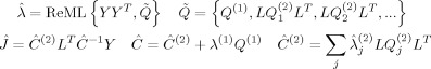APPENDIX B.

Various methods to construct the interpolation matrix H in Eq. (1) have been proposed recently [Andrade et al.,2001; Grova et al.,2006; Kiebel et al.,2000; Operto et al.,2008]. Each row of this matrix can be seen as an interpolation kernel that summarizes the functional information at a particular vertex from a subset of neighboring voxels. The choice of the interpolation kernels depends on the trade‐off between choosing large kernels to account for the spatial extent of the hemodynamic sources, and small kernels, to avoid mixing sources from different anatomical structures. One way to define these kernels is to make them anatomically informed, for example, by taking into account the highly folded nature of the cortical surface. However, the cortical surface that is extracted from a T ₁‐weighted anatomical image usually has different spatial distortions from the functional BOLD‐weighted images (e.g., when using EPI). Thus, a rigid‐body transformation might not be sufficient to coregister the fMRI images with the cortical mesh. It is therefore helpful if the interpolation kernels are robust to small misregistration between the anatomical and functional MRI data. The main interpolation procedures proposed in the literature are as follows:

• Nearest Neighbour interpolation [Saad et al.,2004]: each vertex is assigned the value of its containing voxel. This corresponds to a matrix H in which each row contains 0 except for one 1, corresponding to vertex‐voxel pair.

• Trilinear interpolation [Andrade et al.,2001]: each vertex is assigned a weighted average of its neighboring voxels. Each row of H thus contains only a few nonzero values corresponding to the weights of the trilinear interpolation.

• Voronoï‐based interpolation [Grova et al.,2006]: using a segmentation of the gray matter, a geodesic Voronoï diagram is built using cortical surface's vertices as seeds. Each cell of the diagram is then associated with a particular vertex and contains several voxels; a summary of their values (such as the mean) is assigned to that vertex. This interpolation takes into account the highly convoluted nature of the cortical surface, thanks to the use of geodesic distances when building the Voronoï diagram. This can be seen as an anatomically informed spatial smoothing. Furthermore, Grova et al. [2006] showed that this interpolation is insensitive to small registration errors, and so more robust than the two approaches above. Here, each row of H codes for a given cell of the Voronoï diagram, where the cells are nonoverlapping.

• Anatomically informed kernels [Operto et al.,2008]: these are convolution kernels whose shape and distribution rely on the geometry of the local anatomy. Each kernel is constructed as a weighting of the values of neighboring voxels, and the weights are defined by the combination of two functions: one linearly decreasing along the cortical ribbon in a geodesic way, the other being constant inside the gray matter and canceling out linearly outside. This generates kernels that are overlapping, but can still be written as a particular matrix H.

REFERENCES

- Andrade A,Kherif F,Mangin J‐F,Worsley K,Paradis A,Simon O,Dehaene S,LeBihan D,Poline J‐B ( 2001): Detection of fMRI activation using cortical surface mapping. Human Brain Mapp 12: 79–93. [DOI] [PMC free article] [PubMed] [Google Scholar]
- Ashburner J,Friston KJ ( 2005): Unified segmentation. NeuroImage 26: 839–851. [DOI] [PubMed] [Google Scholar]
- Aubert A,Costalat R ( 2002): A model of the coupling between brain electrical activity, metabolism, and hemodynamics: Application to the interpretation of functional neuroimaging. NeuroImage 17: 1162–1181. [DOI] [PubMed] [Google Scholar]
- Babiloni F,Babiloni C,Carduci F,Angelone L,Gratta CD,Romani GL,Rossini PM,Cincotti F ( 2001): Linear inverse estimation of cortical sources by using high resolution EEG and fMRI priors. Int J Bioelectromagn 3: 62–74. [Google Scholar]
- Baillet S,Garnero G ( 1997): A Bayesian approach to introducing anatomo‐functional priors in the EEG/MEG inverse problem. IEEE Trans Biomed Eng 44: 374–385. [DOI] [PubMed] [Google Scholar]
- Baillet S,Mosher JC,Leahy RM ( 2001): Electromagnetic brain mapping. IEEE Signal Process Mag 18: 14–30. [Google Scholar]
- Bentin S,Allison T,Puce A,Perez E,McCarthy G ( 1996): Electrophysiological studies of face perception in humans. J Cogn Neurosci 8: 551–565. [DOI] [PMC free article] [PubMed] [Google Scholar]
- Berg P,Scherg M ( 1994): A fast method for forward computation of multiple‐shell spherical head models. Electroencephalogr Clin Neurophysiol 90: 58–64. [DOI] [PubMed] [Google Scholar]
- Brookes M,Gibson A,Hall SD,Furlong PL,Barnes GR,Hillebrand H,Singh KD,Holliday IE,Francis S,Morris PA ( 2005): GLM‐beamformer method demonstrates stationary field, α ERD and γ ERS co‐localisation with fMRI BOLD response in visual cortex. Neuroimage 15: 302–308. [DOI] [PubMed] [Google Scholar]
- Calhoun VD,Adali T,Pearlson GD,Kiehl KA ( 2006): Neuronal chronometry of target detection: Fusion of hemodynamic and event‐related potential data. Neuroimage 30: 544–553. [DOI] [PubMed] [Google Scholar]
- Chung MK,Taylor J ( 2004): Diffusion smoothing on brain surface via finite element method. IEEE Int Symp Biomed Imag 1: 432–435. [Google Scholar]
- Dale AM,Sereno M ( 1993): Improved localization of cortical activity by combining EEG and MEG with MRI surface reconstruction: A linear approach. J Cogn Neurosci 5: 162–176. [DOI] [PubMed] [Google Scholar]
- Dale AM,Liu AK,Fishl BR,Buckner RL,Belliveau JW,Dewine JD,Halgren E ( 2000): Dynamic statistical parametric mapping: Combining fMRI and MEG for high‐resolution imaging of cortical activity. Neuron 26: 55–67. [DOI] [PubMed] [Google Scholar]
- Daunizeau J,Grova C,Mattout J,Marrelec G,Clonda D,Goulard B,Pélégrini‐Issac M,Lina J‐M,Benali H ( 2005): Assessing the relevance of fMRI‐based prior in the EEG inverse problem: A Bayesian model comparison approach. IEEE Trans Signal Process 53: 3461–3472. [Google Scholar]
- Daunizeau J,Jbabdi S,Grova C,Mattout J,Marrelec G,Lina J‐M,Benali H ( 2007): Symmetrical event‐related EEG/fMRI information fusion in a variational Bayesian framework. NeuroImage 36: 69–87. [DOI] [PubMed] [Google Scholar]
- Daunizeau J,Vaudano AE,Lemieux L: Bayesian multi‐modal model comparison: A case study on the generators of the spike and the wave in Generalised Spike‐Wave complexes. NeuroImage (in press). [DOI] [PubMed] [Google Scholar]
- David O,Kiebel S,Harrison L,Mattout J,Kilner J,Friston KJ ( 2006): Dynamic causal modelling of evoked responses in EEG and MEG. NeuroImage 30: 1255–1272. [DOI] [PubMed] [Google Scholar]
- Debener S,Ullsperger M,Siegel M,Engel AK ( 2006): Single‐trial EEG‐fMRI reveals the dynamics of cognitive function. Trends Cogn Sci 10: 558–563. [DOI] [PubMed] [Google Scholar]
- Fischl B,Sereno MI,Tootell RB,Dale AM ( 1999): High‐resolution intersubject averaging and a coordinate system for the cortical surface. Human Brain Mapp 8: 272–284. [DOI] [PMC free article] [PubMed] [Google Scholar]
- Flandin G,Penny WD ( 2007): Bayesian fMRI data analysis with sparse spatial basis function priors. Neuroimage 34: 1108–1125. [DOI] [PubMed] [Google Scholar]
- Flandin G,Kherif F,Pennec X,Malandain G,Ayache N,Poline J‐B ( 2002): Improved detection sensitivity in functional MRI data using brain parcelling technique. Proceedings of the 5th MICCAI, LNCS 2488 (Part I), Tokyo, Japan. pp 467–474.
- Friston KJ,Penny W,Phillips C,Kiebel S,Hinton G,Ashburner J ( 2002): Classical and Bayesian inference in neuroimaging: Theory. NeuroImage 16: 465–483. [DOI] [PubMed] [Google Scholar]
- Friston KJ,Harrison L,Penny W ( 2003): Dynamic causal modelling. NeuroImage 19: 1273–1302. [DOI] [PubMed] [Google Scholar]
- Friston KJ,Henson RN,Phillips C,Mattout J ( 2005): Bayesian estimation of evoked and induced responses. Human Brain Mapp 27: 722–735. [DOI] [PMC free article] [PubMed] [Google Scholar]
- Friston KJ,Mattout J,Trujillo‐Barreto N,Ashburner J,Penny W ( 2007): Variational free‐energy and the Laplace approximation. Neuroimage 34: 220–234. [DOI] [PubMed] [Google Scholar]
- Friston KJ,Harrison L,Daunizeau J,Kiebel SJ,Phillips C,Trujillo‐Bareto N,Henson RN,Flandin G,Mattout J ( 2008): Multiple sparse priors for the M/EEG inverse problem. NeuroImage 39: 1104–1120. [DOI] [PubMed] [Google Scholar]
- Gonzalez‐Andino SL,Blanke O,Lantz G,Thut G,Grave de Peralta Menendez R ( 2001): The use of functional constraints for the neuroelectromagnetic inverse problem: Alternatives and caveats unified segmentation. Int J Bioelectromagn 3: 55–66. [Google Scholar]
- Grova C,Makni S,Flandin G,Ciuciu P,Gotman J,Poline J‐B ( 2006): Anatomically informed interpolation of fMRI data on the cortical surface. NeuroImage 31: 1475–1486. [DOI] [PubMed] [Google Scholar]
- Haralick RM,Shapiro LG ( 1992): Computer and Robot vision, Vol. I Addison‐Welsey Longman, Boston, MA: pp 28–48. [Google Scholar]
- Henson RN,Goshen‐Gottstein Y,Ganel T,Otten LJ,Quayle A,Rugg MD ( 2003): Electrophysiological and haemodynamic correlates of face perception, recognition and priming. Cereb Cortex 13: 793–805. [DOI] [PubMed] [Google Scholar]
- Henson RN,Mattout J,Singh K,Barnes G,Hillebrand A,Friston KJ ( 2007): Population‐level inferences for distributed MEG source localization under multiple constraints: Application to face‐evoked fields. NeuroImage 38: 422–438. [DOI] [PubMed] [Google Scholar]
- Henson RN,Mattout J,Phillips C,Friston KJ ( 2009a): Selecting forward models for MEG source‐reconstruction using model‐evidence. Neuroimage 46: 168–176. [DOI] [PMC free article] [PubMed] [Google Scholar]
- Henson RN,Mouchlianitis E,Friston KJ ( 2009b): MEG and EEG data fusion: Simultaneous localisation of face‐evoked responses. Neuroimage 47: 581–589. [DOI] [PMC free article] [PubMed] [Google Scholar]
- Horwitz B,Poeppel D ( 2002): How can EEG/MEG and fMRI/PET data be combined? Hum Brain Mapp 17: 1–3. [DOI] [PMC free article] [PubMed] [Google Scholar]
- Kiebel SJ,Goebel R,Friston KJ ( 2000): Anatomically informed basis functions. NeuroImage 11: 656–667. [DOI] [PubMed] [Google Scholar]
- Kiebel SJ, Daunizeau J, Phillips C, Friston KJ (2008): Variational Bayesian inversion of the equivalent current dipole model in EEG/MEG. Neuroimage 15: 728–41. [DOI] [PubMed] [Google Scholar]
- Kilner JM,Mattout J,Henson R,Friston KJ ( 2005): Hemodynamic correlates of EEG: A heuristic. Neuroimage 28: 280–286. [DOI] [PubMed] [Google Scholar]
- Kobayashi E,Bagshaw AP,Gotman J,Dubeau F ( 2007): Metabolic correlates of epileptic spikes in cerebral cavernous angiomas. Epilepsy Res 73: 98–103. [DOI] [PubMed] [Google Scholar]
- Korvenoja A,Huttunen J,Salli E,Pohjonen H,Martinkauppi S,Palva JM,Lauronen L,Virtanen J,Ilmoniemi RJ,Aronen HJ ( 1999): Activation of multiple cortical areas in response to somatosensory stimulation: Combined magnetoencephalographic and functional magnetic resonance imaging. Human Brain Mapp 8: 13–27. [DOI] [PMC free article] [PubMed] [Google Scholar]
- Lemieux L,Krakow K,Fish DR ( 2001): Comparison of spike‐triggered functional MRI BOLD activation and EEG dipole model localization. NeuroImage 14: 1097–1104. [DOI] [PubMed] [Google Scholar]
- Lin FH,Witzel T,Hämäläinen MS,Dale AM,Belliveau JW,Stufflebeam SM ( 2004): Spectral spatiotemporal imaging of cortical oscillations and interactions in the human brain. Neuroimage 23: 582–595. [DOI] [PMC free article] [PubMed] [Google Scholar]
- Litvak V,Friston K ( 2008): Electromagnetic source reconstruction for group studies. NeuroImage 42: 1490–1498. [DOI] [PMC free article] [PubMed] [Google Scholar]
- Liu AK,Belliveau JW,Dale AM ( 1998): Spatiotemporal imaging of human brain activity using functional MRI constrained magnetoencephalography data: Monte Carlo simulations. Proc Natl Acad Sci USA 95: 8945–8950. [DOI] [PMC free article] [PubMed] [Google Scholar]
- Logothetis NK,Pauls J,Augath M,Trinath T,Oeltermann A ( 2001): Neurophysiological investigation of the basis of the fMRI signal. Nature 12: 150–157. [DOI] [PubMed] [Google Scholar]
- MacKay DJC ( 1995): Probable networks and plausible predictions—A review of practical bayesian methods for supervised neural networks. Network: Comput Neural Syst 6: 469–505. [Google Scholar]
- Mangin J‐F,Frouin V,Bloch I,Régis J,Lopez‐Krahe J ( 1995): From 3D magnetic resonance imaging to structural representation of the cortex topography using topology preserving deformations. J Math Imaging Vision 5: 297–318. [Google Scholar]
- Mangun GR,Buonocore MH,Girelli M,Jha A ( 1998): ERP and fMRI measures of visual spatial selective attention. Hum Brain Mapp 6: 383–389. [DOI] [PMC free article] [PubMed] [Google Scholar]
- Martínez‐Montes E,Valdés‐Sosa PA,Miwakeichi F,Goldman RI,Cohen MS ( 2004): Concurrent EEG/fMRI analysis by multiway partial least squares. Neuroimage 22: 1023–1034. [DOI] [PubMed] [Google Scholar]
- Mattout J,Phillips C,Penny WD,Rugg MD,Friston KJ ( 2006): MEG source localization under multiple constraints: An extended Bayesian framework. NeuroImage 30: 753–767. [DOI] [PubMed] [Google Scholar]
- Mattout J,Henson RN,Friston KJ ( 2007): Canonical source reconstruction for MEG. Comput Intell Neurosci ID67613. [DOI] [PMC free article] [PubMed] [Google Scholar]
- Nunez PL,Silberstein RB ( 2000): On the relationship of synaptic activity to macroscopic measurements: Does co‐registration of EEG with fMRI make sense? Brain Topogr 13: 79–96. [DOI] [PubMed] [Google Scholar]
- Operto G,Bulot R,Anton J‐L,Coulon O ( 2008): Projection of fMRI data onto the cortical surface using anatomically‐informed convolution kernels. Neuroimage 39: 127–135. [DOI] [PubMed] [Google Scholar]
- Phillips C,Rugg MD,Friston KJ ( 2002): Anatomically informed basis functions for EEG source localization: Combining functional and anatomical constraints. Neuroimage 16: 678–695. [DOI] [PubMed] [Google Scholar]
- Phillips C,Mattout J,Rugg MD,Maquet P,Friston KJ ( 2005): An empirical Bayesian solution to the source reconstruction problem in EEG. NeuroImage 24: 997–1011. [DOI] [PubMed] [Google Scholar]
- Penny WD,Stephan KE,Mechelli A,Friston KJ ( 2004): Comparing dynamic causal models. NeuroImage 22: 1157–1172. [DOI] [PubMed] [Google Scholar]
- Riera JJ,Wan X,Jimenez JC,Kawashima R ( 2006): Nonlinear local electrovascular coupling I: A theoretical model. NeuroImage 27: 896–914. [DOI] [PMC free article] [PubMed] [Google Scholar]
- Saad Z,Reynolds C,Argall B,Japee S,Cox RW ( 2004): Suma: An interface for surface‐based intra‐ and inter‐subject analysis with AFNI. Proc IEEE ISBI 1510–1513. [Google Scholar]
- Sotero RC,Trujillo‐Barreto NJ ( 2008): Biophysical model for integrating neuronal activity, EEG, fMRI and metabolism. Neuroimage 39: 290–309. [DOI] [PubMed] [Google Scholar]
- Stephan KE,Kasper L,Harrison LM,Daunizeau J,den Ouden HE,Breakspear M,Friston KJ ( 2008): Nonlinear dynamic causal models for fMRI. Neuroimage 15: 649–662. [DOI] [PMC free article] [PubMed] [Google Scholar]
- Stippich C,Freitag P,Kassubek J,Soros P,Kamada K,Kober H,Scheffler K,Hopfengartner R,Bilecen D,Radu EW,Vieth JB ( 1998): Motor, somatosensory and auditory cortex localization by fMRI and MEG. Neuroreport 9: 1953–1957. [DOI] [PubMed] [Google Scholar]
- Talairach J,Tournoux P ( 1988): Co‐planar stereotaxic atlas of the human brain. Stuttgart: George Thieme Verlag. [Google Scholar]
- Taulu S,Simola J,Kajola M ( 2005): Applications of the Signal Space Separation Method. IEEE Trans Signal Process 53: 3359–3372. [Google Scholar]
- Tipping M ( 2001): Sparse bayesian learning and the relevance vector machine. J Mach Learn Res 1: 211–244. [Google Scholar]
- Trujillo‐Barreto NJ,Martínez‐Montes E,Melie‐García L,Valdés‐Sosa PA ( 2001): A symmetrical Bayesian model for fMRI and EEG/MEG neuroimage fusion. Int J Bioelectromagn 3:ISSN 1456–7865. [Google Scholar]
- Wipf D,Nagarajan S ( 2009): A unified Bayesian framework for MEG/EEG source imaging. NeuroImage 44: 947–966. [DOI] [PMC free article] [PubMed] [Google Scholar]
- Worsley KJ,Marrett S,Neelin P,Vandal AC,Friston KJ,Evans AC ( 1995): A unified approach for determining significant signals in images of cerebral activation. Hum Brain Mapp 4: 58–73. [DOI] [PubMed] [Google Scholar]
- Zhang Z ( 1992): Iterative point matching for registration of free‐form curves and surfaces. Int J Computer Vis 13: 119–152. [Google Scholar]
Associated Data
This section collects any data citations, data availability statements, or supplementary materials included in this article.
Supplementary Materials