Heterogenous Population Coding of a Short-Term Memory and Decision Task

Abstract

We examined neural spike recordings from prefrontal cortex (PFC) while monkeys performed a delayed somatosensory discrimination task. In general, PFC neurons displayed great heterogeneity in response to the task. That is, although individual cells spiked reliably in response to task variables from trial-to-trial, each cell had idiosyncratic combinations of response properties. Despite the great variety in response types, some general patterns held. We used linear regression analysis on the spike data to both display the full heterogeneity of the data and classify cells into categories. We compared different categories of cells and found little difference in their ability to carry information about task variables or their correlation to behavior. This suggests a distributed neural code for the task rather than a highly modularized one. Along this line, we compared the predictions of two theoretical models to the data. We found that cell types predicted by both models were not represented significantly in the population. Our study points to a different class of models that should embrace the inherent heterogeneity of the data, but should also account for the nonrandom features of the population.

Introduction

Neural circuits have the amazing capacity to assimilate information on-the-fly and to perform computations on dynamically stored information (Fuster, 1973; Miller et al., 1991; Kojima and Goldman-Rakic, 1982; Shadlen and Newsome, 2001). The prefrontal cortex (PFC) is believed to be a key area in coordinating cognitive demands involving dynamically stored information (Fuster, 2001; Miller and Cohen, 2001). It is known to show sustained activity in short-term memory tasks (Fuster and Alexander, 1971; Funahashi et al., 1989; Miller et al., 1991), encode reward expectancy (Watanabe, 1996; Leon and Shadlen, 1999), and integrate stimulus identity and location (Fuster et al., 1982; Rao et al., 1997). Given its myriad functions, it comes as no surprise that PFC neurons should have complex response properties (Miller, 1999).

Delayed discrimination tasks require the rapid storage of information in short-term memory followed by a computation in which this memory, in combination with a current sensory stimulus, is used to inform decisions about action. One set of experiments (Romo et al., 1999; Romo and Salinas, 2003) has previously looked at the neural signature of such a memory-to-action transformation in macaque monkeys performing a delayed somatosensory discrimination task. Neurons recorded from PFC (Romo et al., 1999), medial premotor cortex (MPC) (Hernández et al., 2002) and ventral premotor cortex (VPM; Romo et al., 2004) showed activity correlated to stimulus values, memory, and decision outcome. In other words, they showed activity related to the entire memory-to-decision transformation.

Previous reports of these PFC data during the delayed vibrotactile discrimination task have described it during the first stimulus (f1) and delay periods (Romo et al., 1999; Brody et al., 2003). Here, we have two major goals. First, we report on the neural spike data in PFC during the f2/decision period, paying particular attention to the relationship between neuronal response properties during f2 and response properties during the delay period and f1. Across the population, PFC displays a great heterogeneity in the response property relationships. We will, despite this, also emphasize the many regularities in the data.

Our second goal is to examine how well the specifics of response property distributions match two previous, competing, computational models of the memory-to-decision transformation in this task. These two models were devised by disjoint subsets of the current authors, and make clearly distinct predictions and assumptions about neural response properties. Using uniform criteria across the two models, we analyze the data from PFC to examine how many recorded neurons satisfy the criteria laid down by each of the models.

Finally, in the Discussion section, we consider possible modular architectures with which to model these data. None of the modular architectures we consider seems to fit the data well. We conclude that nonmodular circuits, in which information representation is spread across neurons in a multiplexed manner, may be the best direction to explore in future models.

Materials and Methods

Behavioral task.

The behavioral task has been reported previously (Romo et al., 1999; Romo and Salinas, 2003). Briefly, the task requires comparing two vibrotactile frequencies, separated by a fixed 3 s delay, and applied sequentially to a fingertip (see Fig. 1A). The subject must report a binary decision about whether the f1 had a higher, or lower, vibration frequency than the second stimulus (f1>f2? Y or N). That is, to perform the task, the subject must a) perceive and represent the value of frequency f1; b) store the value of f1 in short-term memory during the delay period; and c) compare the second stimulus value (f2) to the one stored in memory, resulting in a binary decision.

Figure 1.

The behavioral task and our standard neural data analysis method. A, Behavioral task. Monkeys are presented a brief vibrotactile stimulus (f1) (yellow background), followed by a 3 s delay (DEL), and then another brief stimulus (f2) (light green background). After the end of the second stimulus, the subject chooses a pushbutton to report their answer to the question “f1>f2? Yes or No.” B, Stimulus sets. Monkeys are trained using a variety of frequency pairs. The two most common frequency sets are shown; only one set is used in any given session. Within each panel, the presence of a gray box indicates an (f1,f2) frequency pair used in the experiment. The background color indicates the appropriate response (Y or N) to that pair. Different pairs in a set are presented in pseudorandom order during the session. C, Neural data analysis. Given that each trial type is defined by the (f1,f2) stimulus values, we analyze neural firing rates as a function of f1 and f2. For each time slice t, each neuron's firing rate r(t) is expressed as a linear function of f1 and f2, by regressing r(t) = b₁(t) f₁ + b₂(t) f₂ + b₀(t). Each dot shows the values of b₁(t) and b₂(t) for one neuron; panels show five selected time slices. A dot lying on the horizontal axis indicates a neuron whose firing rate depends only on f1; a dot on the vertical axis indicates a neuron whose firing rate depends only on f2; and a dot lying on the b₁ = −b₂ diagonal indicates a neuron whose firing rate depends only on the value of f1−f2. Since the subject's decision depends on the sign of f1−f2, neurons whose firing rate depends on f1−f2 can be easily used to compute the appropriate decision. Dot color indicates whether the neuron can be interpreted as f1-dependent only (green), f2 dependent only (blue), or (f1−f2)-dependent (red; see Materials and Methods). Open black circles indicate neurons not significantly different from the origin, whereas open magenta circles indicate significantly different from origin, but not falling into any of the green, blue, or red classes. Ellipses represent a Gaussian fit to the population data. The angle of the ellipse, measured as the clockwise rotation of the major axis relative to the horizontal, is indicated in the upper right corner.

Regression.

Before f2 is presented, we model the spike rate of each neuron as follows:

where r(t) is the value of the PSTH at time t and a₀ is the baseline regressor and a₁ is the f1 regressor. We call (1) the reduced model. The full model is described by the following:

where b₀ is the baseline regressor, b₁ is the f1 regressor, and b₂ is the f2 regressor. The full model (2) applies after the onset of f2, from ST2 and beyond. PSTHs were constructed in a way such that only spikes within an epoch are included in its calculation, and PSTHs were calculated at 25 ms intervals.

The firing rate of some neurons in this dataset is better fit with a linear function followed by a sigmoidal nonlinearity (Brody et al., 2003), see supplemental Methods, available at www.jneurosci.org as supplemental material. However, our main focus in this paper is on the firing rate dependence on f1 and f2, namely, the b₁ and b₂ parameters, and in particular, the direction of the vector formed by b₁ and b₂.

As we show in the supplemental Methods (available at www.jneurosci.org as supplemental material), the direction of this vector is very similar for the purely linear (Eq. 2) and the sigmoidal fits (see supplemental Fig. S3 and supplemental Eq. S1, available at www.jneurosci.org as supplemental material). None of the qualitative conclusions of the paper change if we use sigmoidal as well as purely linear fits. For simplicity and for consistency in fitting all neurons in the same way, we report here the results using linear fits.

Significance of regression.

For the reduced model, each value of the time-dependent regression coefficient, a₁(t) was considered significant if it passed a t test at p < 0.01. Significance for the full model is more complicated because the location of the regression on the b₁-b₂ plane must be considered. More specifically, we must consider the uncertainty in the regression point which will be an ellipsoid specified by the joint confidence region (JCR) given as follows:

(Draper and Smith, 1981) where F(·) is the 1-α (e.g., 0.95 or 0.99) percentile of the F-distribution with p = 3 parameters and ν = N_T − p degrees of freedom, where N_T is the number of trials (data points) used in the regression. The time-dependent value s²(t) = (ξ^T(t)ξ(t))/(N_T′p) is an unbiased estimate of the variance, where ξ(t) = Xb^T(t) − r(t) is the residuals from regression (assumed to be independently, identically, and normally distributed). The column vector b(t) = [b₀(t) b₁(t) b₂(t)]^T is the center of the ellipsoid in the coordinates described by β = [β₀ β₁ β₂]^T. X is the regression model given by the following:

where the matrix has a row for all N_T trials and where the bars over f1 and f2 indicated the mean values across all trials for the given cell.

Since we are interested in finding the significance of the b₁ and b₂ coefficients only, we set β₀(t) = b₀(t). In other words, the ellipsoid surface defined in (3) is projected as an ellipse in the β₁-β₂ plane. The boundary can be reduced to the following quadratic equation:

where K_α ≡ ps²(t)F(p, ν, 1 − α), Δβ_j ≡ β_j, and

for j = 1, 2 and

We want to test whether each regression point is significantly different from the origin and significant to f1, f2, or f1−f2. This is accomplished by testing whether each regression point obeys or violates (4) under each condition. For significance from the origin, we set β₁ = β₂ = 0 and tested (4) at the 99% confidence level, i.e., α = 0.99. For significance to f1, f2, or f1−f2, we must test (4) to the lines defined by β₁ = 0 (see Fig. 1C, horizontal green line), β₂ = 0 (see Fig. 1C, vertical blue line), and β₁ = −β₂ (see Fig. 1C, diagonal red line) respectively. In order for a point to be considered significant to a line, it must obey (4) at the 95% level for one of the lines, and violate (4) at the 99% level for the other two lines. In other words, a point must regress significantly close to one of the lines at the 95% confidence level, but must regress far from the other lines at the 99% confidence level. We also tested significance to the line β₁ = β₂. However, due to the shape of most JCRs—an ellipse with the major axis perpendicular to this line—and due to the crowding of significance lines, we did not require exclusivity to this line. Therefore, it is possible for a point to be simultaneously significant to f1 or f2 and f1+f2.

Categorization.

Using the individual significances of each bin, we applied a uniform criteria for both models to determine the encoding type of each cell. We used the regression analysis described above and applied a set of thresholds on the number of bins where the f1 regressor and/or the f2 regressor was significantly different from zero for each task epoch. Significance of regression coefficients for each bin was determined using the methods described above in Significance of Regression.

For the f1 period and the delay period, i.e., before f2 is presented, we used the regression model defined in (1) and counted the number of bins where the f1 regressor a₁(t) was significantly different from zero. After f2 presentation, we applied the model defined in (2) and counted the number of bins where the f1 regressor b₁(t) and the f2 regressor b₂(t) (we will henceforth drop the explicit reference to time dependence in the coefficients) significantly regressed to f1, f2, f1−f2 (comparison), or f1+f2; see Significance of regression above for details.

PSTHs for categorizations were generated by convolving spike trains with a Gaussian kernel with SD 50 ms during f1 and f2 periods and 150 ms during the delay period. PSTHs were sampled every 25 ms. Gaussian kernels were truncated and normalized at task epoch boundaries; therefore, for example, spikes from the f1 presentation could not contribute to f1 significance to a bin located in the delay period.

For the f1 period, a cell was considered f1-sensory encoding if a₁ was significant (p < 0.01) in more than half of the bins (>5/10) in the middle 250 ms of f1 stimulus presentation (125–375 ms). The cell was called positively (negatively) f1-sensory encoding if a₁ > 0 (a₁ < 0) in all bins where a₁ was significant. If any of the significant bins had opposite signs, we labeled the cell as sign-switching. Using this criteria, we found that 361/912 (179 negative, 171 positive, 11 sign-switching) cells were categorized as f1-sensory encoding during the f1 stimulus period. Shuffling f1 labels in the regression produced 3/912 (2 negative, 1 positive, 0 sign-switching) cells categorized as f1-sensory encoding during the f1 stimulus period.

The situation for the delay is more complicated because cells show time-dependent activity related to f1 (Brody et al., 2003). Therefore, we broke up the delay period into six sections of 500 ms each (20 bins per section). To be called f1 memory encoding, a cell had to have a₁ be significant in more than half of the bins (>10/20) in one or more of the six sections. Positive (negative) f1 memory encoding cells were defined as those where a₁ > 0 (a₁ < 0) in all bins where a₁ was significant. If any of the significant bins had opposite signs, we labeled the cell as sign-switching. Using this criteria, we found that 455/912 (198 negative, 240 positive, 17 sign-switching) cells were categorized as f1 memory encoding during the delay period. Shuffling f1 labels in the regression produced 28/912 (17 negative, 11 positive, 0 sign-switching) cells categorized as f1 memory encoding during the delay period.

In addition to defining cells as explicitly f1 memory encoding during the delay, we are also interested in finding cells that are explicitly not f1 memory encoding during the delay. Therefore, we looked for cells whose a₁ were not significantly different from zero (p > 0.01) in >80% of bins (>16/20) in all six segments of the delay period. We found 358/912 cells categorized as explicitly not f1 memory encoding during the delay period. Shuffling f1 labels in the regression produced 837 of 912 cells categorized as explicitly not f1 memory encoding during the delay period.

During the second stimulus, the monkey receives f2 so we must consider that the activity of cells can encode some combination of f1 and f2. Knowing whether the regression coefficients, b₁ and b₂ from the regression model (2), are significantly different from zero does not provide enough information; a cell can regress to an ambiguous mixture of f1 and f2 (see Significance of Regression above). We want to know specifically whether each cell's activity regresses significantly to f1, f2, or f1−f2. We therefore tested the significance of regression coefficients using the joint confidence regions of b₁ and b₂ as described in Significance of regression above.

In general, it is more difficult to meet the significance criteria established for the full (f1,f2) regression model (2). Therefore, we lowered the threshold in the number of significant bins. For a cell to be f1 memory encoding during the f2 stimulus period, a cell had to significantly regress to f1 in >20% (>2/10) of bins during the middle 250 ms of the f2 stimulus period (125–375 ms of f2 presentation). Similarly, for a cell to be f2-sensory encoding, a cell had to significantly regress to f2 in >20% (>2/10) of bins during the middle 250 ms of the f2 stimulus period. For a cell to be comparison encoding, a cell had to significantly regress to f1−f2 in >20% (>2/10) of bins during the middle 250 ms of the f2 stimulus period. And for a cell to be f1+f2 encoding, a cell had to significantly regress to f1+f2 in >20% (>2/10) of bins during the middle 250 ms of the f2 stimulus period. Cells could be considered encoding more than one of the above at different times. For example, a hypothetical cell that had 3 bins significant to, say, f1 from 125 to 200 ms into f2 presentation and later had 4 bins significant to, say, f1−f2 from 275 to 375 ms would be considered both f1 memory encoding and comparison encoding. Determining sign of the regression is similar as in earlier epochs. A cell is called positive (negative) f1 memory encoding during f2 presentation, if b₁ > 0 (b₁ < 0) in all f1-significant bins. If b₁ had opposite signs in f1-significant bins, the cell was called sign-switching. A similar criteria held for f2-sensory encoding cells, with positive (negative) sign for b₂ > 0 (b₂ < 0) in all f2-significant bins. For comparison encoding, sign was positive (negative) for b₁ − b₂ > 0 (b₁ − b₂ < 0) in all comparison significant bins. Note: positive comparison encoding cells prefer trials where f1 − f2 > 0, i.e., “yes” trials; negative comparison encoding cells prefer trials where f1 − f2 < 0, i.e., “no” trials. And for f1 + f2 encoding activity, sign was positive (negative) for b₁ + b₂ > 0 (b₁ + b₂ < 0) in all comparison significant bins. Using this criteria, we found: 79 of 912 (28 negative, 51 positive, 0 sign-switching) f1 memory-encoding cells during the f2 stimulus period, 117/912 (48 negative, 69 positive, 0 sign-switching) f2-sensory encoding cells, 398/912 (216 negative “no”, 178 positive “yes”, 4 sign-switching) comparison encoding cells, and 74 (10 negative, 15 positive, 49 sign-switching) f1 + f2 encoding cells. Shuffling (f1,f2) labels in the regression produced: 1 of 912 (1 negative) f1 memory encoding cells during the f2 stimulus period, 0 of /912 f2-sensory encoding cells, 0 of 912 comparison encoding cells, and 1 of 912 (1 negative) f1 + f2 encoding cells.

For Figure 5, cells labeled “memory and decision” were the intersection of all cells that were f1 memory encoding during the delay and comparison encoding during f2 presentation; cells labeled “decision only” were all other comparison encoding cells.

Figure 5.

Comparison between memory and decision cells (purple) and decision only cells (green). A, Snapshots of the regression coefficients for 4 different time intervals. Each point is a cell. Ellipses are the 2-σ fit of a weighted Gaussian. B, Angle as a function of time for the entire task. The 45° line (upper dashed line) represents the decision line, where activity is related to the difference between f1 and f2. C, The behavioral ACP (ability to discriminate correct and error trials based on spike count) of the two populations. D, Spike count discriminability (ability to discriminate between correct “yes” and “no” trials) of the two populations. In A, C, and D, shaded regions represent 95% confidence intervals measured from bootstrapping.

For Figure 7, cells were counted into the different types by finding the intersection of cells that fit the stimulus encoding predictions of each model. For example, the Machens, Romo, Brody model predicts a cell type that has positive f1-sensory encoding during f1 presentation, positive f1 memory encoding during the delay, and “yes” (positive, i.e., +f1−f2) comparison encoding during the f2 stimulus period (see Fig. 7A, left). To count the number of cells matching this model, we found cells that met all three criteria.

Figure 7.

Schematic and accounting of different cell encoding types. A, The two MRB cell types. Schematic of the model is shown on the left. The two trajectories show an idealized diagram for how the regression coefficients change in the three task epochs. Numbers beside dots indicate the epoch (see the legend at the bottom right corner of A). Below each trajectory, a diagram of how the color encoding should unfold in time, as in Figure 3A, for each cell type. Above each trajectory, numbers indicate the total from the population categorized into the archetype. Numbers to the side indicate the total. Conventions used in panel A hold for all panels. B, The two MW comparison cells without memory. C, The two MW memory cells. D, The two MW comparison cells with memory. E, Four types not predicted by either model but discovered in the data.

Simplified categorization.

The above set of strict criteria can separate neurons into very specific categories at the expense of culling cells whose encoding are more ambiguous. To generate a more inclusive set of criteria, we placed one of three labels separately for each epoch for each cell. During the f1 stimulus period and separately for the delay, we labeled each cell as positive or negative f1 encoding or nonencoding. For the f2 stimulus period, we labeled each cell as “yes” or “no” decision encoding or non-decision encoding. A single significant bin would place a cell as encoding for that epoch whereas a nonencoding cell would need to have zero significant bins in the entire epoch. To decide whether a cell was positive or negative (“yes”-decision or “no”-decision) encoding, we used a simple majority between the two encoding types; the majority of cells encode variables with a uniform sign throughout each epoch) (see Fig. 3). During the f2 period, we were only deciding whether cells encoded the difference f1−f2 (f2−f1) or not. During this period, cells can encode f1, f2, or some different combination of both; the simplified categorization does not attempt to differentiate between these encoding types.

Figure 3.

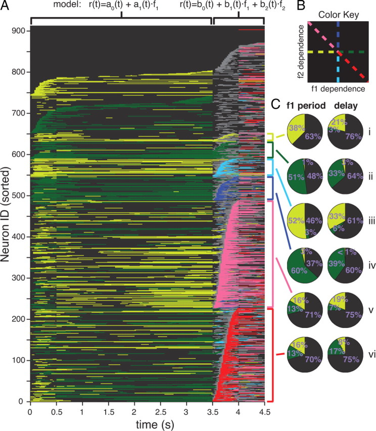
Overview of task encoding in all 912 cells. A, Significance of regression as a function of time for all 912 PFC considered in this study. Each row represents a cell. Color encodes significance to one of the lines as indicated in the key shown in B. Black indicates not significantly different from the origin; gray indicates significantly different from the origin but ambiguous to any of the lines; green (green-yellow), blue (sky blue), red (pink) indicate significant encoding of f1 (−f1), f2 (−f2), and f1−f2 (−f1+f2), respectively. Neurons are sorted by the timing of different colors in different epochs, see main text. The sorting generates natural groups which are indicated by the colored brackets to the right of the plot. Different regression models are used before the onset of the f2 stimulus, indicated at the top of the plot. B, Color key used A. C, Pie charts show the fraction of total bins occupied by each color during the f1 period (left) and delay (right) for each bracketed group.

Population angle.

To obtain the angle of the population of regression points, we want to calculate the underlying (assumed normal) population distribution. Each regression point itself, however, is drawn from a probability distribution which depends on such factors as the stimulus set used during the experiment and the amount of noise in the data. Therefore, calculating the population distribution can be done by calculating the maximum likelihood estimate of the posterior distribution of the population, assuming that the individual probability distributions are priors. Specifically, we assume that each observed point is the result of the sum of two probability distributions, one known from the regression, the other unknown from the population:

where b_n and σ_n refer to the mean and the covariance of the prior probability distributions as obtained from regression and the subscript indexes neuron n, and B and Γ refer to the mean and covariance of the unknown posterior distribution. To obtain the latter quantities, we maximize the following log-likelihood function:

with respect to B and Γ. There are a number of methods to accomplish this, but we chose to directly maximize the log-likelihood using a simplex algorithm as implemented in Matlab (MathWorks Inc.). We confirmed that a gradient descent algorithm provides results consistent with the simplex method. To ensure that the optimization would not produce “unphysical” results, e.g., negative covariance or determinant, we artificially introduced a high value for the log-likelihood in those neighborhoods with a gradient that pushed the algorithms toward physically consistent values. To obtain confidence intervals for the angles, we performed a bootstrap using 10,000 randomly resampled with replacement configurations of the population.

Behavioral average choice probability.

We want to compare neurons that have both f1 memory during DEL and f1−f2 activity during ST2 to those that have no memory during DEL and have f1−f2 activity during ST2, see Categorization above. More specifically, we want to know which group of cells is better correlated with behavior. For this, we calculate the average choice probability in spike rate between correct and error trials. In other words, we ask what percentage of correct trials can we successfully classify by comparing spike rates in both conditions? For example, for a neuron that spikes at high rates when f1>f2, i.e., a “yes” neuron (see Fig. 2), one expects it will spike at a lower rate on error trials where f1>f2 and spike at a higher rate on error trials where f1<f2; one has the opposite expectation for “no” neurons. Therefore, the first step in calculating the average choice probability (ACP) is classifying each cell by its decision preference. For the cells of interest here, this has already been done during the categorization of cells. We then calculate the ACP of cell n and stimulus pair k using the following:

where N_c and N_e are the number of correct trial and error trials respectively, r_c,i(t) and r_e,j(t) are the i^th correct and j^th error trial spike rate as a function of time respectively, and θ(.) is the Heaviside-Theta function, defined as follows:

The exponent δ_n,k controls the sign of the argument to the Heaviside-Theta function and is determined by the decision encoding of the cell and the trial type, i.e., whether f1>f2 or f1<f2. It is defined as follows:

which is to say, correct trials should have higher spike rates for “yes'” neurons when f1>f2 and for “no” neurons when f1<f2, and correct trials should have lower spike rates for “yes” neurons when f1<f2 and “no” neurons when f1>f2.

Figure 2.

Individual cells show diversity in response to stimuli. Trajectories of regression coefficients are shown in the top, PSTHs, averaged across correct trials for each (f1,f2)-stimulus pair, are shown in the bottom. For regression trajectories, each point is a time bin (sampled every 200 ms), lines show the full smooth trajectory (sampled every 50 ms). The shape of each point encodes the task epoch as indicated by the key in panel A, Color encodes significance of regression to the associated dotted lines, e.g., dark green indicates the cell's activity regressed significantly to +f1; black indicates not significantly different from the origin; gray indicates significantly different from origin but ambiguous compared with all lines (see Materials and Methods). For PSTHs (bottom), light yellow background indicates f1 presentation whereas light-green background indicates f2 presentation. In all panels, line color encodes f1 frequency for all times before f2 presentation; the color key is shown on the bottom right panel. After f2 onset, in A, B, D, and E, colors smoothly transition into coding the correct answer for each trial type: gray-blue for f1>f2? yes trials, gold for f1>f2? no trials. In C, line colors encode f1 throughout. In E, line colors transition into a code for f2 after f2 onset. Below PSTHs, the colored bars indicate regression significance using the same color scheme as in the top. Points directly above the bar indicated the same points plotted in the top using the same color and shape scheme. A, Cell showing persistent f1 activity in the f1 period and delay, followed by comparison activity during the f2 period. B, Cell showing no significant stimulus activity until the f2 period, where it shows comparison related activity. C, Cell showing only f1-related activity early and late in the task, even into f2 presentation. D, Cell showing f1 activity during the f1 period, nothing during the delay, followed by comparison activity during the f2 period. E, Cell similar to the one shown in A, however, its trajectory is different in that it prefers to spike higher for “no” trials than in “yes” trials. F, Cell showing f1 activity during the f1 period and delay, followed by f2 activity during the f2 period.

Monkeys can perform the task with an accuracy above 90%; therefore, ACP is a very noisy quantity at the single neuron level. Indeed, some neurons are recorded during sessions where the monkey does not make a single error; the ACP is ill-defined for those cases. Therefore, ACP is averaged over all stimulus pairs over all neurons in a given population. Confidence intervals are obtained by bootstrapping the neural population 10,000 times.

Spike rate discriminability.

The behavioral average choice probability attempts to correlate a neuron's spike rate with behavior using correct and error trials. We also want to compute how easily an ideal observer could categorize spike rates in trials where f1>f2 (“yes”) versus trials where f1<f2 (“no”); we do this for correct trials only. Ideally, one could use a measure like d-prime to describe the “distance” between two distributions. However, d-prime applies to distributions that are completely described by mean and variance. Therefore, we use the average choice probability to calculate spike rate discriminability (SRD).

We segregated all firing rates from “yes” trials and “no” trials for each neuron using only correct trials. To eliminate the effects of f1 memory activity, we used trials from stimulus pairs where f1 was matched in the “yes” and “no” trials, see middle six stimuli of Figure 1B (left). We then calculated the SRD of neuron n using the following:

where N_Y and N_N are the number of “yes” and “no” trials respectively, r_Y,i and r_N,j are the i^th “yes” and j^th “no” trial spike rate respectively, and θ(·) is again the Heaviside-Theta. The exponent δ_n controls the sign of the arguments to the Heaviside-Theta function, and is determined by the decision encoding of neuron n using the following:

We then bootstrap the “yes” and “no” trials 10,000 times and calculate the SRD based on the resampled trials. The SRD for neuron n is the median value from the bootstrap, and single neuron confidence intervals are based on the single neuron bootstrap. When the SRD of a population is calculated, the median of the single neuron bootstrap is used for each neuron. The population itself is then resampled 10,000 times to obtain a bootstrap of the medians of the population.

Results

The transformation from sensory representation to graded memory of the sensory stimulus to decision can be seen at the population level. It is apparent in the orientation of the ellipse in Figure 1C, which describes the f1 and f2 dependence of the population for five different time intervals as indicated above each panel. During the first stimulus period (Fig. 1C, left) neurons respond primarily to the value of the incoming frequency as shown by the spread along the horizontal axis, demonstrating firing rate dependence on f1. This representation is maintained during the delay period (second and third panels from left) which shows the memory of f1 in the population. During the second stimulus period (fourth and fifth panels), neurons begin to show activity related to the comparison between f1 and f2; the population rotates to the line 45° below horizontal, indicating activity related to the difference between f1 and f2.

The averaged population-level view described above obscures the complex dynamics that individual neurons display. The dynamics of each neuron can be very reliable from trial to trial, even while there is great heterogeneity across neurons. Figure 2 illustrates the dynamics of 6 different representative neurons. Some neurons show stimulus-dependent activity throughout all task periods. Other neurons show stimulus-dependent activity only during a portion of each trial (cf. Fig. 2B with other panels). Furthermore, the nature of the stimulus dependence can vary greatly from neuron to neuron. For example, the neuron in Figure 2C shows activity that depends only on the value of f1; the f1-dependent activity starts during the f1 period, disappears during the middle portion of the delay, reemerges at the end of delay, and continues into the presentation of f2. In contrast, the neuron of Figure 2B shows stimulus-dependent activity only during the f2/decision period; this neuron's response is bimodal, and highly correlated with the animal's choice at the end of the trial.

In terms of their stimulus encoding, neurons with linear coefficients indicating a +f1−f2 dependence (Figs. 2 and 3, dark red) or −f1+f2 (Figs. 2 and 3, pink) are directly linked to the animal's decision in the sense that the task involves computing the sign of (f1−f2). Neurons that encoded this difference, of either sign, are then neurons with firing rates that are directly correlated with the appropriate behavioral choice on each trial. In contrast, neurons with a response during the f2/decision period that encode f1 only, or f2 only, do not allow a direct choice readout.

We attempt to portray the full heterogeneity of the neural data by analyzing each neuron individually and presenting the results for the entire population. As before, each neuron's firing rate was regressed to stimulus values. From the regression coefficients and their associated confidence regions, we then classified each time point into 8 possible categories, illustrated by the color code in the upper inset of Figure 3B. For presentation clarity, we used two different regression models for different parts of the task, as indicated at the top Figure 3A. Briefly, before f2 presentation, we used a reduced model where we only considered a regression to the value of f1 (a₁(t)) plus a constant term (a₀(t)). After f2 presentation, we use the full regression model as described earlier in the text and in Materials and Methods. The result of the regression determines the color of each time interval for each cell. If the regression at time interval t_i was not significantly different from the origin (a₁(t_i) = 0 for the reduced or b₁(t_i) = b₂(t_i) = 0 for the full model), the time interval was colored black. If the regression point was significantly different from the origin, than they were labeled using the following scheme: positive f1 (dark green), negative f1 (light green), positive f2 (dark blue), negative f2 (light blue), f1−f2 (red), f2−f1 (pink), and if the point was different from the origin but could not be unambiguously assigned to any of the preceding lines (gray). The reduced regression model eliminates ambiguous points—hence, no gray bins before f2 onset; regression points and associated confidence intervals lie along a line, and therefore they either overlap the origin or they do not and instead are positive or negative.

Using this color scheme, we could illustrate the stimulus dependence of each neuron as a function of time. Each cell is placed on its own horizontal row of colored bins with time progressing from left to right, and the color of each time interval representing the cell's encoding during that time point. The results of analyzing every neuron in this manner are shown in Figure 3A. Neurons were further sorted and sub-sorted by the timing of their encodings. The first six sorting criteria was earliest time of f1−f2, f2−f1, +f2, −f2, +f1, −f1 during the f2/decision period respectively; the sorting criteria naturally produces six groups of neurons—indicated by the colored brackets.

The largest two groups are composed of neurons that are decision-correlated during the f2/decision period, encoding either +f1−f2 (“yes”) (dark red, n = 25%, 227/912) or −f1+f2 (“no”) (pink, n = 29%, 261/912). We examined the average encoding of each of these groups during the f1 period and during the delay period (Fig. 3Cv, vi). Most of these decision-correlated neurons did not encode f1 during the f1 period or delay (black in main panel and in pie charts). However, for those decision-correlated neurons that do show f1 encoding during the delay, a pattern in the encoding relationship between delay period and f2/decision period emerges: +f1−f2 decision-correlated neurons tend, by a factor of 2:1, to spend their time encoding +f1 during the delay (Fig. 3Cvi, right), whereas −f1+f2 decision-correlated neurons tend to encode −f1 during the delay (Fig. 3Cv right). Given that the transition from the f1 period to the delay period shows a relatively low number of encoding sign switches (Romo et al., 1999), we might expect a similar relationship to hold between the first stimulus period and the second stimulus/decision period. Nevertheless, this is not the case: both groups of decision-correlated neurons spend equal time encoding +f1 as −f1 during the f1 stimulus period (Figs. 3Cv left, vi).

Two groups of neurons respond to the second stimulus, f2, in a manner predominantly dependent on f2 only (Fig. 3A, dark blue and light blue). Of these neurons, those encoding +f2 predominantly encode +f1 during the f1 period (Fig. 3Civ left); conversely, those encoding −f2 predominantly encode −f1 during the f1 period (Fig. 3Ciii left). These neurons might thus appear to be purely sensory neurons, responding only to the current stimulus in a manner consistent across the two stimulus periods. However, to our surprise, we found that a very high fraction of these “quasisensory” neurons also encode f1 during the delay period (Fig. 3Ciii, Civ right), thus showing a strong short-term memory response in addition to their sensory responses. Although relatively small in number, of all the groups we studied, the quasisensory group of neurons spent the highest fraction of time encoding f1 during the delay period, suggesting that this category of cells might be particularly important for maintenance of short-term memory.

Two more groups of neurons were those formed by neurons encoding f1, the first stimulus, during f2, the second stimulus. These neurons, like the sensory driven neurons described above, maintain their sign of encoding throughout the task. For example, the +f1 cells (dark green) have 51% +f1 encoding during f1 presentation and 33% +f1 encoding during the delay versus 1% and 3% to −f1 respectively (Fig. 3Cii). The −f1 cells (light green) maintain 38% and 21% −f1 encoding versus 0% and 3% +f1 encoding during f1 presentation and delay respectively (Fig. 3Ci).

Finally, near the top of the Figure 3A, starting at neuron 651, we sorted all other cells based on their first time of +f1 and −f1 significance during the f1 period and delay, followed by the first time of ambiguous encoding in the f2/decision period. Quite a few cells show significance to +f1 and −f1 (91 and 62 neurons respectively) during limited portions of the task; many other cells show ambiguous significance during f2/decision but not during any other time (67 neurons starting at 804).

While we have described some of the gross trends observable in Figure 3A, we note here some of the finer details. These generally indicate the high level of heterogeneity in response properties across neurons. We point out three such properties. (1) Within each of the bracketed response groups during the f2/decision period that we defined, we further sub-sorted the neurons vertically according to the latency of the onset of their response category. In supplemental Fig. 1A–C, available at www.jneurosci.org as supplemental material, we show the distribution of all decision significant time intervals for all cells in the dark red and pink groups (A), the median of the decision time for each cell (B), and the first decision time (C); the distributions are broad indicating that cells become decision related throughout the f2/decision period. Taking neurons that encode +f1-f2 (dark red) as an example, some neurons acquire their +f1−f2 encoding almost as soon as f2 is presented—although one should not, from this fact, conclude that cells are making the discrimination immediately since spikes are convolved with Gaussian kernels—whereas other neurons encode +f1−f2 only toward the end of stimulus f2. A similar wide spread in latencies can be observed for the other groups in Figure 3A. (2) In addition to latencies being widely different across neurons, so are the durations of the period of time over which the neurons encode the decision, observable in Figure 3A as the various horizontal extents of encoding in different cells. (3) At different points in time, even looking only within the f2/decision period, different neurons encode different stimulus properties. For example, a few neurons encode −f1 during the delay and start of the f2/decision period, but then encode −f2, and only later encode +f1−f2 (neuron numbers 145–150). Many different such patterns are visible. Some of the most remarkable are neurons that invert their encodings: as can be seen in Figure 3A, some neurons encode +f1−f2 (dark red), but later reverse themselves, encoding −f1+f2 (pink); the converse also occurs, with neurons encoding f2−f1 (pink) and later +f1−f2 (dark red). We emphasize that the patterns thus described are not simply noise: Figure 3A shows only the encodings that are highly significant (see Significance of regression in Materials and Methods).

In Figure 4A, we show the average PSTH of each group from Figure 3A. The “decision”-related groups, Figure 4Ai, show strong binary activity depending on whether the trial was f1>f2 or f1<f2. In contrast, the +f2 and −f2 groups, Figure 4Aii, show graded activity during the f2/decision period. The +f1 and −f1 groups, Figure 4Aiii, show graded activity related to f1 during the beginning of the f2/decision period, but then segregate between yes and no trials toward the end; however, rather than a purely binary spike rate as in Figure 4Ai, activity is graded based on the (f1,f2) combination.

Figure 4.

Activity and average choice probability for all cells by group. A, Average PSTHs of all cells within a group broken up by frequency. The rainbow color code indicates the value of the f1 stimulus during the f1 and delay periods, and for panel Aii only, indicates the value of the f2 stimulus during the f2/decision period. B, Average choice probability of all cells within a group broken down by cells with memory activity during the delay and those without. Shaded regions represent 95% confidence intervals based on bootstrapping. Black lines show median values of the entire population regardless of category. Dotted brown lines show chance performance for visual reference.

To quantify the correlation between spike rate and behavior for each group, we computed the behavioral ACP for each neuron and averaged the values in each group. Figure 4B shows the results. Within each of the six groups, neurons were further subdivided by whether they possessed f1 memory during the delay. Across all six groups, neurons encoding f1 have a higher-than-chance ACP at the end of the delay period (purple traces), consistent with these neurons being part of the neural substrate used to hold the short-term memory of f1. But after the f2 stimulus begins, the different groups show very different properties. Neurons encoding +f1−f2 or −f1+f2, Figure 4Bi, show very high ACP, consistent with their being involved in computing the choice that the subject will subsequently report with its behavior. Furthermore, only the +f1−f2 memory cells, Figure 4Bi left, showed a significant difference in ACP from the non-memory cells during f2 presentation (p < 0.01, random permutation test). Neurons encoding +f2 or −f2, Figure 4Bii, show ACP indistinguishable from chance after f2 onset, even for those memory-carrying neurons that had higher than chance ACP values before the onset of f2. Neurons in the +f1 and −f1 groups, Figure 4Biii, do show an increase in the ACP after f2 onset, however the increase is less pronounced than in the “yes” and “no” groups, compare with Figure 4Bi. The difference in the ACP of the two populations is evident from the PSTHs, Figure 4Ai and Aiii. The “yes” and “no” cells spike in a strong binary pattern during the two different trial categories, whereas the +f1 and −f1 cells spike in a graded pattern.

Figure 4 hints at some differences between cells that carry memory related activity during the delay period and those that do not. In Figure 4Bi, memory cells from the “yes” group show an elevated ACP during the second stimulus period compared with those with no memory. On the other hand, cells from the “no” group do not show a difference between the two populations. To further examine this relationship, we disregarded the group structure from Figure 3 and simply categorized cells into two groups: memory and decision cells and decision only cells. We used strict criteria (see Materials and Methods) to ensure that only those cells with significant decision and memory related activity are included in the analysis thereby reducing noise from cells that show marginal or transient significance. Memory and decision cells outnumber decision only cells 225 to 173. To determine whether one group becomes associated with the decision faster than the other, we calculated the regression angle of both populations separately using a weighted Gaussian fit, see Materials and Methods. Figure 5A shows snapshots of the two population regressions at four different time intervals. By the first 100 ms of the second stimulus turning on, neither population has moved toward the 45° decision line. Just 70 ms later, however, both populations have begun to rotate, reaching the 45° line somewhere between 275 to 300 ms after f2 onset. Figure 5B shows the population angle as a function of time. Neither population reaches the decision line clearly before the other. We also tested the correlation of the activity with the behavioral choices of the monkey for both populations (Fig. 5C). The memory and decision population appears to be greater than the decision only population. We found that the difference between the means in the second half of the f2 period was significant with p = 0.0176 using a random permutation test with 10,000 shuffles of labels between memory and non-memory cells. The ACP measures spike activity relative to behavioral performance. We also tested the theoretical discriminability of spike rates between “yes” trials and “no” trials using correct trials only (Fig. 5D). Again, we found that memory cells elevated versus their non-memory counterparts. The difference between means in the second half of the stimulus period was highly significant (p < 0.001).

Comparison of data with existing models

Two competing computational models, by distinct subsets of the current authors, have proposed different mechanisms by which neural circuits could achieve the memory-to-decision transformation displayed in the current data. Both the Machens-Romo-Brody (MRB) model (Machens et al., 2005) and the Miller-Wang (MW) model (Miller and Wang, 2006) have assumed that PFC is the locus of both the memory of f1 and the discrimination between f1 and f2. But the mechanism differs in the two models, leading to different predictions for how the core computational cells encode task variables. Given the great diversity of responses seen in PFC, e.g., in Figure 3, we asked how well supported are each of the models in the data—that is, we ask what fraction of cells observed in the data fit the predicted response characteristics described by each model. Below, we first describe an overview of the stimulus encoding found in the data (Fig. 6). We then summarize the basic properties of each of the two models, and describe the cell classes that each model predicts. We then make the comparison between models and data (Fig. 7).

Figure 6.

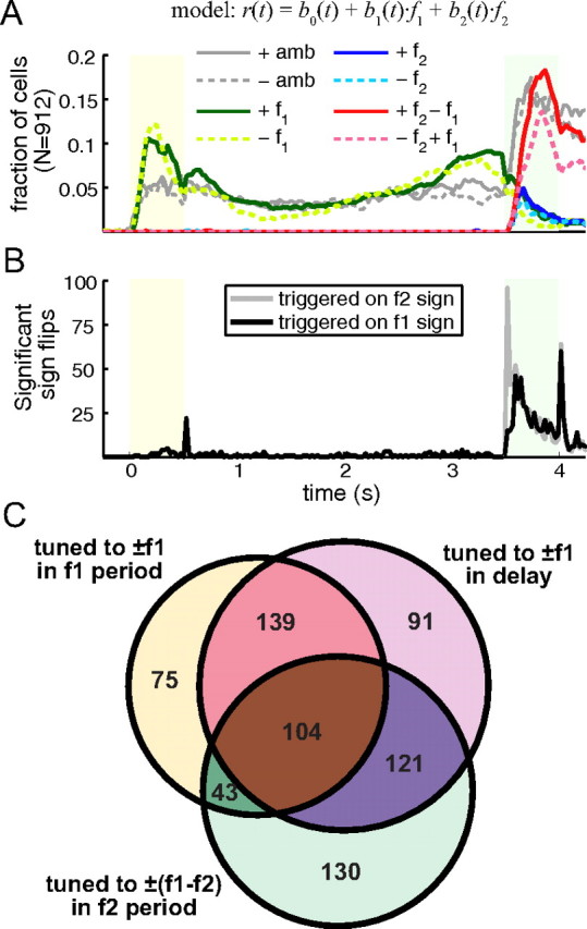
Overview of stimulus encoding in the population. A, Fraction of cells in the population showing significant regression to stimuli broken down by type and sign. Color scheme is identical to the one used in Figure 3. Gray lines before f2 onset appear here because the full regression model is used for the whole task. This was done to show the relative representation of f1 and the comparison in the population using the same criteria. B, Number of significant sign flips as a function of time. C, Venn diagram showing the number of cells categorized as: f1-sensory encoding during f1 presentation (circle containing yellow segment), f1 memory encoding in the delay (circle containing lavender segment), comparison encoding during f2 presentation (circle containing light green segment), and the combination of intersections between all three categories. Numbers in each segment are exclusive.

To examine this question, we need to categorize the activity of each cell to stimulus values. We again apply our standard regression analysis using strict criteria to ensure that cell responses are robust to task stimuli. In this analysis, we will focus on how cells change encoding signs from one task epoch to another; e.g., if a cell encoded +f1 during the first stimulus period does it remain positive during the delay or switch signs to become negative or possibly lose f1 encoding altogether? Since the models have different predictions for f1-sensory, f1 memory, and comparison encoding in PFC cells, we may be able to disambiguate the two models from the evidence in the data.

In Figure 6, we show an overview of stimulus encoding in the population. Figure 6A shows the total fraction of cells that have significant regression coefficients (see Significance of regression in Materials and Methods) broken down by stimulus type and sign as a function of time. In essence, Figure 6A is a summary of Figure 3 showing the total fraction of cells in each color for every time bin. However, in Figure 6A we used the full regression model for the entire task rather than just after the second stimulus. We did this to show more clearly how the representation of the comparison (solid red and dashed pink lines) is stronger than the representation of f1 during the first stimulus presentation and delay (solid dark green and dashed light green lines). In comparing the two models, we will be emphasizing transitions in encoding signs from one epoch to another. Figure 6B shows an overview of the number of significant transitions that occur throughout the task. Anytime a cell regressed significantly different from the origin at one time interval then switched sign significantly at a later time interval, we counted that as a sign switch at the latter time. In Figure 6B, very few of the sign switches occur before the onset of the second stimulus. After second stimulus however, many cells switch signs. Interestingly when the sign switch is triggered on the f2 sign (gray line), a large peak at the beginning of the f2 period appears. When the switch is triggered on f1 (black line), however, there is no initial sharp peak; after a short delay the number of flips rises to f2 levels and falls with it to the end of the f2 period. Another interesting feature is the sharp peak for both lines after the f2 period. Many cells reverse their decision encoding, e.g., from f1−f2 to f2−f1, during this time; this is also evident in Figure 3 where many cells in the red group turn pink and cells in the pink group turn red between 4 and 4.5 s.

When comparing the two models, we required that cells be significant over extended periods in each epoch; something that cannot be gleaned from Figure 6A alone. Therefore, we applied a strict criteria to the number of time bins that a cell has significant regression coefficients to categorize encoding types (see Categorization in Materials and Methods). Figure 6C shows a Venn diagram depicting the intersection of three categories of cells: (1) f1-sensory encoding during the f1 stimulus period, (2) f1 memory encoding during the delay, and (3) comparison encoding during the f2 stimulus period. By category, 361/912 (40%) of cells were f1 sensory encoding, 455/912 (50%) of cells were f1 memory encoding, and 398/912 (44%) of cells were comparison encoding. There are 703/912 (77%) cells that fit into at least one category and are shown in Figure 6C. Of these, many neurons were counted in one category but not in any of the others (296/703, 42%). Many neurons were counted in some combination of two of the categories (303/703, 43%). A smaller number of neurons fit into all three categories (104/703, 15%). As a comparison, if one randomly shuffles the three categories for all 912 cells, the expected number of cells fitting at least one category is 756, with 377/756 (50%) of cells fitting only a single category, 300/756 (40%) of cells fitting two categories, and 79/756 (10%) of cells fitting all three categories. We performed a Pearson's χ² test that the percentage of cells fitting exactly one, exactly two, and all three categories are different from the null random expected values. We found that all three percentages were significant with p-values of 5.3E-6, 0.0048, and 6.0E-4 for exactly one, two, and three categories respectively. The significance of our findings suggests that being in one category is correlated with being in another category, more than expected by chance. In other words, we found more combined f1-sensory encoding, f1 memory encoding, and comparison encoding than expected by chance. We note here that in Fig. 6A, the fraction of cells with significant regression to the decision is much higher than the fraction of cells with significant regression to f1 during the delay at any given time. However, the number of cells categorized as f1 memory encoding during the delay is comparable to the number of cells categorized as comparison encoding during the second stimulus period. This is primarily due to differences in regression models (and associated significance analysis) used for the two periods. Also, since the delay period is longer and cells can be memory encoding during anytime of the delay, there are more opportunities to be categorized as an f1 memory encoding neuron. However, the categorization is not simply due to noise as we had strict requirements for inclusion in each category. Also, shuffling stimulus pair labels for the regression produced very few cells in each category: 3/912 for f1-sensory encoding during the f1 period, 28/912 for f1 memory encoding during the delay, and 0/912 for comparison encoding during the f2 period. We tested a number of different criteria for categorization (data not shown), with little difference to the general trend of the data presented here and in the comparison of the two theoretical models that follows.

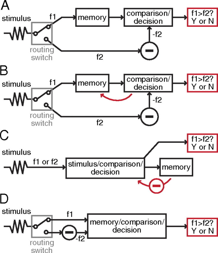
With the overall picture in hand, we now turn to the specifics of the two theoretical models. The two models predict distinct neural signatures that would be observed using the analysis tools of Figure 1C. As we will describe below, the MRB model predicts the presence of 2 neural signatures, and the MW model predicts the presence of 6 signatures. No class belongs to both models, and we therefore expect that determining which classes predominate in the data should allow us to distinguish between the models. We now discuss each of the predicted signatures in turn.

A key assumption of the MRB model is that the same set of PFC neurons both encode the memory of f1 during the delay and perform the binary comparison during f2. The core of the MRB model is a demonstration of how a single neural circuit in PFC, with a fixed architecture, can accomplish both graded persistent activity and binary decision-making. In this model, the populations of cells that have positive monotonic encoding of f1 (“plus” cells) and those that have negative monotonic encoding (“minus” cells) mutually inhibit one another to form a line attractor circuit (Seung, 1996) during the delay period. A decrease in tonic excitation to such a circuit transforms it from a line attractor, capable of graded persistent activity, to a bistable circuit, capable of binary decision-making. This dual capacity is a result of the mutual inhibition architecture. Thus, in the MRB model both the plus and the minus populations are required for the system's operation.

Although the circuit within PFC is fixed in the MRB model, the connections from sensory areas to PFC do change. The MRB model depends on the assumption that a within-trial switch in effective connectivity between sensory areas and PFC exists. That is, the effective connectivity from secondary somatosensory cortex (S2) to PFC must change in sign at some time from the f1 to the f2 period. Machens et al. (2005) observed that most neurons that are plus during the delay subsequently fire most during f2 in trials where f1>f2, i.e., they encode f1−f2 (“yes” decisions; see Fig. 3vi right). This means that during f2, the lower the value of f2, the higher the firing rate, which is the opposite of the stimulus dependence observed during the delay period. Thus, the sign of the dependence on the sensory stimulus had switched from plus to minus. Similarly, neurons that are minus during the delay also display a sign switch, but in the opposite direction (see Fig. 3v right). This experimental observation, combined with the observation that few neurons change the sign of their encoding from f1 presentation to delay, led to the postulate that between the f1 period and the f2 period, there should be a switch in the sign of the effective connectivity between sensory areas and PFC. The MRB model was constructed based on the assumption that this postulate was correct. Biophysically, such a switch could be accomplished using either a context-dependent signal and an inhibitory switch in S2 (Machens et al., 2005), or by using appropriately chosen, fixed synaptic weights from S2 to PFC (Chow et al., 2009).

In the MRB model, then, neurons that are plus (minus) f1-sensory encoding during f1 presentation should remain plus (minus) f1 memory encoding during the delay and become f1−f2 (“yes”) comparison encoding during f2 presentation. Such neurons, if analyzed using the standard method illustrated in Figure 1C, would display the dynamics diagramed in Figure 7A, left (plus) and right (minus).

Struck by the inelegance of requiring a within-trial sign switch in effective connectivity from sensory areas to PFC, and motivated by considering the existence of such a switch implausible, Miller and Wang (2006) devised a competing model in which no switch or connectivity change is required anywhere in the circuit. In contrast to the MRB model, the MW model uses two separate neural populations for the memory and the comparison/decision operations. Sensory stimuli from S2 drive a population of comparison/decision cells (labeled “C” cells), which in turn drive a bank of cells capable of graded memory (“M” cells, configured as a line attractor/integrator). The M cells perfectly integrate incoming signals from the “C” cells and in turn provide negative feedback to the “C” cells. An f1 sensory stimulus thus causes an increase in the activity of “C” cells, which in turn causes an increase in the activity of “M” cells, and this increase continues until the activity of the “M” cells has grown to the point where their negative feedback to the “C” cells exactly cancels the sensory input. At this point the “C” cells no longer drive an increase in “M” cell activity. When the sensory stimulus turns off, the “M” cells continue to fire persistently at a rate that depends on the value of the previously presented f1 stimulus. The “M” cells thus encode a memory of f1 throughout the delay. The “C” neurons are inhibited by the “M” neurons and hence are quiescent. During f2, sensory stimuli driving the “C” cells will encounter the incoming stimulus input and the continuing negative feedback from the “M” cells which is in proportion to the memory of f1. Thus, “C” cells will only respond to f2 if it is sufficiently large to overcome the negative feedback. That is, the “C” cells only fire if f2>f1. As a result, these cells in the MW model perform the f1 versus f2 comparison without requiring any switch in effective connectivity.

If analyzed using the standard method of Figure 1C, the “C” cells would be driven into “plus” activity during f1; the inhibition from the “M” cells would silence the “C” cells again by the end of f1, leading the “C” cells to have no encoding during the delay; finally, during f2 these cells would fire when f2 is greater than f1. A diagram of the dynamics of such “C” cells is shown in Figure 7B left. “M” cells analyzed in the same way would become “plus” during f1 presentation, remain “plus” during the delay, and then during f2 would fire in a manner that increased as a function of f1+f2; this is illustrated in Figure 7C left.

The MW model does not strictly require having both a “plus” and a “minus” population. Nevertheless, the model can be constructed in either the “plus” configuration or in the “minus” configuration. Furthermore, having both configurations greatly facilitates the final readout of the decision. Thus the MW model also predicts activity patterns diagramed in Figure 7, B and C right, which are the “minus” circuit versions of Figure 7, B and C left.

As described thus far, the MW model does not account for neurons that change the sign of their stimulus-dependency from the delay to f2. Miller and Wang observed that their model could be modified to account for such cells by having some of the integrator “M” cells ignore inputs below a minimum threshold θ. This has the advantage of increasing the robustness of the “M” cell integrator. The MW model further proposes that throughout each trial, a tonic input drives “C” cells to fire at θ. Thanks to this input, an extra input from the f1 stimulus drives the “C” cells to a firing rate above the “M” cell threshold, therefore affecting the “M” cells and leading to the negative integral feedback process: the negative feedback from the “M” cells would increase until it brought the “C” cells back to the firing rate θ, thus canceling the f1 input. After this, when the f1 input ceases at the end of the first stimulus period, the “M” cells continue firing at a rate proportional to f1, thus holding the f1 memory; and the inhibitory input from the “M” cells, combined with the lack of the f1 sensory input and the tonic excitation, drives the “C” cells to a firing rate proportional to θ − f1. That is, the sign of the “C” cell encoding to f1 switches from “plus” during f1 to “minus” during the delay. When f2 is presented, “C” cells will be initially driven to a firing rate proportional to θ + (f2 − f1). Thus values of f2 that are greater than the previously presented f1 will lead “C” cells to fire above θ, whereas values of f2 less than f1 will lead the “C” cells to fire below θ. The “C” cell firing rate can therefore be used to form the appropriate decision (f1 > f2? Y or N), with θ forming the decision boundary. Using again the tools of Figure 1C, the “plus” circuit version of these “C” cells is illustrated in Figure 7D left, and the “minus” circuit version is illustrated in Figure 7D right.

In summary, the analysis tools of Figure 1C lead us to seek 2 different signatures compatible with the MRB model (Fig. 7A) and 6 different signatures compatible with the MW model (Fig. 7B–D). No class belongs to both models, and we therefore expect that determining which classes predominate in the data should allow us to distinguish between the models. We analyzed the firing rates of 912 recorded neurons and classified each into the eight different classes defined in Figure 7A–D. Additionally, we classified cells into categories not predicted in either model, Figure 7E–H.

Categorization was based on regression and significance analysis. Details can be found in Materials and Methods. Briefly, for the two stimulus periods, we require that at least half of the time bins within the middle 250 ms have significant regression coefficients with all significant bins having the same encoding sign. For the delay period, we divided the 3 s into 6 equal 500 ms segments. Within each segment, we required that at least half of the bins regressed significantly and were of the same sign. If any one segment passed criteria, we defined the cell as having memory. Cells with multiple segments passing criteria would also need to have all signs be identical. For situations where cells were required specifically to not encode any stimuli, we set a lower threshold for the number of significant bins which a cell had to be under to pass. Regressions for this analysis was performed on PSTHs created using a Gaussian kernel with a SD of 50 ms during stimulus periods and 150 ms during all other times. Gaussians were truncated and normalized for edge effects at epoch boundaries. Therefore, for example, memory of f1 during the delay is not attributable to convolving spikes from the stimulus periods. In our analysis, we do not consider the temporal dynamics of each neuron. In principle, the MRB and MW models rely on fixed-points to maintain f1 memory encoding during the delay period. Therefore, average firing rates should remain steady throughout the delay. Many cells, however, show strong temporal dynamics which are reliable on a trial-to-trial basis. To simplify our analysis, we did not attempt to define cells based on temporal characteristics.

Figure 7 shows the total number of cells conforming to each cell type at the top of each panel and the total for each model along the sides of the panels. Overall, only a small fraction of cells (80/912, 9%) fit into one of the eight categories outlined above for both models. Of those, a total of 47 fit into the MRB model categories whereas a total of 33 fit into the MW model categories. The two numbers that are most readily comparable in this analysis are between the MRB neurons of Figure 7A and the MW “C” neurons with memory of Figure 7D. These cells have the most similar set of criteria, differing only in the signs of the combinations of encodings. When these two sets are compared, the MRB model has the same 47 cells, whereas the MW model has 19 cells. Thus, the MRB model, based on these numbers alone, would appear to be better represented in the data.

One might be concerned that the paucity of numbers reported here are due to overly zealous selection criteria or that if the statistical power on all cells were increased that we may have found more favorable accounting for each model. To demonstrate that this is not the case, in Figure 7, E–H, we show 8 cell categories that are not predicted by either the MRB or the MW models. The numbers for these categories were generated using the same set of criteria used for both models and can be compared with one another. For example, purely sensory cells, Figure 7, E and F, account for 45 cells that show f1 activity during the first stimulus and delay followed by f2 activity during the second stimulus and account for 31 cells that show f1 activity throughout the entire task. A few categories that show decision related activity but are not predicted by either model are shown in Figure 7, G and H. Of these, a small number, 17, show activity like MRB cells during f1 and the delay, but then show decision activity opposite to that predicted by the model. A far greater number, 77, show no stimulus related activity throughout the f1 and delay period, but then show decision related activity during f2.

The 16 categories shown in Figure 7 are only a sample of the total possible categories. In the supplemental Material, Table S1 (available at www.jneurosci.org) shows the numbers of cells that fit into all possible categories, including those enumerated here, and using the same strict categorization criteria throughout. This procedure leads to a well defined category for 568/912 (62%) neurons. The remaining 344 (38%) neurons cannot be unambiguously categorized with these methods.

Therefore, as a second approach, we applied a simpler set of categorization criteria (see supplemental Fig. S4, available at www.jneurosci.org as supplemental material). During the f1 period and separately for the delay period, we placed one of three labels on each cell: positive f1-encoding, negative f1-encoding, or nonencoding. During the f2 period, we used the following three labels: “yes” decision-encoding, “no” decision-encoding, and non-decision-encoding (but could encode f1 or f2), see Materials and Methods for more details. The three labels in three epochs provides 27 nonoverlapping encoding combinations. Two combinations represent neurons that are most similar to the predictions of the MRB model (Fig. 7A); a total of 105 of 912 neurons (12%) best fit this profile (46 of the 105 best fit the left panel of Fig. 7A, whereas the remaining 59 best fit the right panel). Two combinations represent neurons that are most similar to the “C” cells without memory in the MW model (Fig. 7B); a total of 32/912 neurons (4%) best fit this profile (24 of the 32 best fit the left panel, whereas the remaining 8 fit the right panel). Two combinations represent neurons that are most similar to the “C” cells with memory in the MW model (Fig. 7D); a total of 55/912 neurons (6%) best fit this profile (28 of the 55 best fit the left panel, whereas the remaining 27 best fit the right panel). These numbers can be compared with two unpredicted decision cell types shown in Figure 7, G and H. A total of 61/912 neurons (7%) best fit the profiles shown in Figure 7G (29 of the 61 best fit the left panel, whereas the remaining 32 best fit the right panel). A total of 81/912 (9%) neurons best fit the profiles shown in Figure 7H (43 of the 81 best fit the left panel, whereas the remaining 38 best fit the right panel). Supplemental Figure S4 (available at www.jneurosci.org as supplemental material) reports the number of cells that best fit each of the 27 combinations, including the ones described above. It also replots Figure 3 by showing the neurons sorted according to the simplified categorization scheme described above.

In this analysis, of all the cells showing decision related behavior, the two MRB profiles had the highest number of cells that best fit their encoding combinations. However, the numbers were only a few percent higher than other leading categories. Also, the simplified categorization has the disadvantage of underestimating nonencoding categories—a single bin of significance places a cell as encoding in this set of criteria—which is a disadvantage for the MW “C” neuron without memory (Fig. 7B). Note that this is an unavoidable problem as determining nonencoding is not simply the negative of determining encoding; there is a substantial middle ground where cells may show weak or barely significant encoding. Nevertheless, together with the more stringent set of criteria, we conclude that the cell types predicted by either model do not dominate the data. This suggests a highly heterogeneous code in PFC for solving the task.

Given the heterogeneity found in the data, can we constrain future models of this task? Figure 8 sketches the outlines of four circuit architectures that could solve the task. In Figure 8A, the set of neurons supporting short-term memory of f1 is separate from those supporting the comparison between f1 and f2 and/or the formation of the binary decision. The scenario is simple in the sense that each module, or group of neurons, has a single, fixed, and well defined computation. In this scenario, we would not expect memory neurons to carry binary decision-related signals, nor would we expect decision-related neurons to carry memory signals. Neurons with these properties are found in the experimental data. Figure 6C shows 91 neurons that are stimulus-sensitive only during the delay and 130 neurons that are stimulus-sensitive only during f2 presentation; they might be the basis of the circuit sketched in Figure 8A. Other neuronal types (e.g., neurons that are stimulus-sensitive during both the delay and f2 presentation) might be epiphenomenal with respect to the current task and driven by the neurons fully compatible with Figure 8A. Such a view predicts that neurons carrying both memory and decision-related signals, i.e., the “epiphenomenal” cells, should have lower average choice probability (ACP) than those carrying purely memory signals during the delay and purely decision signals during f2. In Figure 5, we compared the ACP of memory and decision cells to non-memory and decision cells; we found ACP favors memory and decision cells during f2. To test the former prediction, we calculated the ACP during the delay period for memory-only cells and memory and decision cells. In supplemental Figure S1 (available at www.jneurosci.org as supplemental material), we show the ACP as a function of time within the delay; we further break down the population of cells based on when they show significant memory activity: early (0–1 s of delay only), middle (1–2 s of delay only), late (2–3 s of delay only), persistent (entire delay), and all others (anything remaining from the above). No difference between the two populations (memory only vs memory+decision) are apparent; again, if anything, the memory+decision cells have a higher ACP when the memory component is persistent. The data, therefore, suggests the scenario of Figure 8A unlikely.

Figure 8.

Schematic of several possible architectures capable of performing the stimulus/memory/comparison transformation required in the task. A, A network that completely separates memory and comparison/decision. B, Similar to A, except that feedback from comparison/decision feeds back onto the memory population creating decision related information in those cells that is epiphenomenal. C, The Miller-Wang model. D, The Machens-Romo-Brody model.

A variation on the scenario of Figure 8A is shown in Figure 8B. Once again the memory module and the comparison/decision module are kept separate, except that once the decision is formed, the result is fed back to the memory module, thus leading to neurons that carry both memory and decision information, as commonly observed in the data. In the scenario of Figure 8B, such feedback is not necessary for the circuit to perform the task; the purpose of the feedback could be related to other tasks that the prefrontal cortex participates in. Nevertheless, if such feedback were present, the 225 neurons (of 912 neurons, 25%) that have both memory and decision-related activity could be accounted for. In such a scenario, we would expect decision-related activity to arise slightly earlier in decision-only neurons than in memory-and-decision neurons, since the former drive the latter. Furthermore, we would expect decision-only neurons to have higher choice probability than memory-and-decision neurons, since they would be more closely linked to the circuit's decision output. Yet, Figure 5 shows precisely the opposite of these two predictions, namely, that memory-and-decision neurons have higher choice probabilities and shorter decision latencies than decision-only neurons. For these reasons, we consider the scenario of Figure 8B unlikely.

Discussion

In this paper, we focused on the phenomenology of neural firing rates in PFC during a two-interval, two-alternative forced-choice task where subjects must compare two vibrotactile frequencies presented serially with a delay. Subjects must use short-term memory to perform the task well above chance. As described in the Introduction and the Results, each trial of the task is composed of three distinct periods (Fig. 1A): (1) the “f1 period”, lasting 500 ms, during which the first stimulus is presented; (2) a “delay period”, lasting several seconds, over which the subject must store the value of f1 in a graded memory; (3) the “f2/decision period”, lasting 500 ms, during which a second stimulus (f2) is presented, and during which the subject compares the f2 stimulus to its memory of f1. At the end of the f2/decision period, the subject chooses to press one of two pushbuttons to indicate its answer to the question “f1>f2? Yes or No.”

Understanding the neural mechanisms by which subjects complete the task requires understanding the circuits by which it is implemented. Although much data has been collected, even broad outlines of the connectivity between functional elements of these circuits remain undetermined.

In our analysis of the scenarios depicted in Figure 8, we found that the data suggests it is unlikely that PFC divides the task into a pure “memory module” and a pure “comparison/decision” module. Instead, neurons carrying memory of f1 in the task are likely to be involved in computing the comparison between f1 and f2. Two competing proposals for models that would combine memory and comparison/decision have been put forward. In the MW model (Fig. 8C), the memory module was segregated, but there is a stimulus/comparison module that receives feedback from the memory module and therefore shows combined responses. In the MRB model (Fig. 8D), memory and comparison/decision are integrated into a single module. We counted how many cells recorded experimentally had response properties that corresponded to the specific predicted properties of each model (MW model: Fig. 7B–D; MRB model: Fig. 7A). Neither model predicted firing properties of a large fraction of the recorded neurons; we found that comparable numbers of cells were classified into types not predicted by either model, suggesting that the neural representation of the task is significantly more heterogeneous than either model postulates. To confirm our results, we performed a simplified categorization on the population (supplemental Fig. S4, available at www.jneurosci.org as supplemental material) and found similar results.

Comparing the models only against one another, we observe numbers slightly in favor of MRB over MW. In particular, we found that the number of cells fitting the “M” population in the MW model was relatively small. This suggests that should the brain use an integrated feedback mechanism to maintain short-term memory as postulated in the MW model that it may reside in a portion of PFC not recorded in our dataset or in an entirely different area. Our data indicates that the encoding of the task is distributed among many different categories, suggesting a heterogeneous code in PFC for solving the task.

Figure 3 is consistent with this view of a highly heterogeneous representation of task variables. Nevertheless, neuronal response properties are not random, and some general patterns are found. Some include: First, cells having higher firing rates in the comparison/decision period for “f1>f2? YES” trials (“yes cells”) tend to be positive monotonic for f1 during the delay period, i.e., their firing rate is higher for higher values of f1 during the delay. In mirror symmetry to “yes” cells, “no” cells tend to be negative monotonic for f1 during the delay. However, this relationship between decision-related responses during the comparison/decision period and memory-related responses to f1 during the delay does not extend back into the f1 stimulus period: both “yes” and “no” cell groups are equally likely to have been positive or negative monotonic during f1. Second, a small but significant fraction (17%) of cells in PFC encode only memory and stimulus information, and do not encode the comparison/decision. Some of these cells do not respond to f2, but simply carry f1 information throughout all three task periods. The others change to encoding f2 during f2 presentation. At first sight, such cells might be good candidates for a pure “memory only” module. However, as noted above, their choice probability values (supplemental Fig. S1, available at www.jneurosci.org as supplemental material) are lower than memory+decision neurons, indicating that they are further removed from performance of the task.

Compared with previous studies of decision-making, our focus in this discussion and in Figure 8 has been on how information held in short-term memory and current stimulus information can be combined in forming a binary decision. We have not focused on the decision-making process itself, in part because our data do not easily permit such a focus: during each of the two sensory stimulus periods, information about the stimulus was delivered relatively quickly, and the decision was performed well above psychometric threshold (the difference |f1−f2| was typically large, and performance on all trial types was correspondingly high, typically >90% correct). In contrast, previous prominent research focusing on the binary decision-making process has often used a single stimulus as a source of information, delivered the information slowly during that stimulus, and used stimuli at or near psychometric threshold. An example is the well known random dots task (Newsome et al., 1989). Neural responses recorded during this random dots task in both PFC (Kim and Shadlen, 1999) and lateral intraparietal area (Roitman and Shadlen, 2002) of monkeys have been approximated with a drift-diffusion model in which the stimulus biases a random walk toward one of two boundaries (Gold and Shadlen, 2007). Contact with a boundary represents making a decision. In this model, the value of the single sensory stimulus is represented by a single parameter (drift rate). The question of how such a biased random walk model should be adapted to make decisions based on information about two stimuli, one incoming and the other held in short-term memory is a very interesting one. Unfortunately, it is not a question that would be well addressed with the dataset examined here, and is therefore outside the scope of this paper.

Decision-making based on a combination of information held in short-term memory and current stimuli has been previously explored in delayed match-to-sample tasks (Miller et al., 1991). Stimuli in these tasks typically are images and hence reside in high-dimensional spaces, i.e., there is no simple analog representation of the image through the graded firing rate of a single neuron. In the task analyzed here, monkeys needed to compare the frequency between two sequentially presented stimuli. Frequency is a one-dimensional analog value; therefore, the brain could potentially adopt a very different strategy to encode and operate on stimuli in these two tasks. Nevertheless, our results, suggesting that memory and decision are intermingled, are compatible with the results of Miller and colleagues, in which neurons with short-term memory activity also showed “match suppression” and “match enhancement” in the decision period.

In this article, our analysis focused on single-neuron properties across various phases of the task, and we compared these single-neuron properties to predictions from two competing theoretical models. We attempted to show, with the greatest amount of detail possible, the full heterogeneity inherent in the firing rates of PFC neurons. This method is in contrast to the common practice of averaging across populations or showing only a few exemplar cells. Many theoretical models are hand-designed with only the exemplars in mind. Our analysis showed that the high level of heterogeneity displayed across different neurons makes comparisons to the simplified models challenging, and in general does not strongly support either model. A different approach might ask whether a simpler representation exists at the level of whole neuronal populations and be expressed heterogeneously at the level of single neurons. Singh and Eliasmith (2006) used such a view to construct a distributed and heterogeneous representation of neuronal responses in this task during f1 and the delay period. Machens et al. (unpublished observations) used a similar view to derive a simplified, data-driven representation, again during f1 and the delay period. Future work will attempt to derive simplified population-level representations that can also account for data during the comparison/decision period. The present analysis describes the single-neuron trends in the data that will constrain future models.

References

- Brody CD, Hernández A, Zainos A, Romo R. Timing and neural encoding of somatosensory parametric working memory in macaque prefrontal cortex. Cereb Cortex. 2003;13:1196–1207. doi: 10.1093/cercor/bhg100. [DOI] [PubMed] [Google Scholar]
- Chow SS, Romo R, Brody CD. Context-dependent modulation of functional connectivity: secondary somatosensory cortex to prefrontal cortex connections in two-stimulus-interval discrimination tasks. J Neurosci. 2009;29:7238–7245. doi: 10.1523/JNEUROSCI.4856-08.2009. [DOI] [PMC free article] [PubMed] [Google Scholar]
- Draper N, Smith H. Ed. 2. New York: Wiley; 1981. Applied regression analysis. [Google Scholar]
- Funahashi S, Bruce CJ, Goldman-Rakic PS. Mnemonic coding of visual space in the monkey's dorsolateral prefrontal cortex. J Neurophysiol. 1989;61:331–349. doi: 10.1152/jn.1989.61.2.331. [DOI] [PubMed] [Google Scholar]
- Fuster JM. Unit activity in prefrontal cortex during delayed-response performance: neural correlates of transient memory. J Neurophysiol. 1973;36:61–78. doi: 10.1152/jn.1973.36.1.61. [DOI] [PubMed] [Google Scholar]
- Fuster JM. The prefrontal cortex—an update: time is of the essence. Neuron. 2001;30:319–333. doi: 10.1016/s0896-6273(01)00285-9. [DOI] [PubMed] [Google Scholar]
- Fuster JM, Alexander GE. Neuron activity related to short-term memory. Science. 1971;173:652–654. doi: 10.1126/science.173.3997.652. [DOI] [PubMed] [Google Scholar]
- Fuster JM, Bauer RH, Jervey JP. Cellular discharge in the dorsolateral prefrontal cortex of the monkey in cognitive tasks. Exp Neurol. 1982;77:679–694. doi: 10.1016/0014-4886(82)90238-2. [DOI] [PubMed] [Google Scholar]
- Gold JI, Shadlen MN. The neural basis of decision making. Annu Rev Neurosci. 2007;30:535–574. doi: 10.1146/annurev.neuro.29.051605.113038. [DOI] [PubMed] [Google Scholar]
- Hernández A, Zainos A, Romo R. Temporal evolution of a decision-making process in medial premotor cortex. Neuron. 2002;33:959–972. doi: 10.1016/s0896-6273(02)00613-x. [DOI] [PubMed] [Google Scholar]
- Kim JN, Shadlen MN. Neural correlates of a decision in the dorsolateral prefrontal cortex of the macaque. Nat Neurosci. 1999;2:176–185. doi: 10.1038/5739. [DOI] [PubMed] [Google Scholar]
- Kojima S, Goldman-Rakic PS. Delay-related activity of prefrontal neurons in rhesus monkeys performing delayed response. Brain Res. 1982;248:43–49. doi: 10.1016/0006-8993(82)91145-3. [DOI] [PubMed] [Google Scholar]
- Leon MI, Shadlen MN. Effect of expected reward magnitude on the response of neurons in the dorsolateral prefrontal cortex of the macaque. Neuron. 1999;24:415–425. doi: 10.1016/s0896-6273(00)80854-5. [DOI] [PubMed] [Google Scholar]
- Machens CK, Romo R, Brody CD. Flexible control of mutual inhibition: a neural model of two-interval discrimination. Science. 2005;307:1121–1124. doi: 10.1126/science.1104171. [DOI] [PubMed] [Google Scholar]
- Miller EK. The prefrontal cortex: complex neural properties for complex behavior. Neuron. 1999;22:15–17. doi: 10.1016/s0896-6273(00)80673-x. [DOI] [PubMed] [Google Scholar]
- Miller EK, Cohen JD. An integrative theory of prefrontal cortex function. Annu Rev Neurosci. 2001;24:167–202. doi: 10.1146/annurev.neuro.24.1.167. [DOI] [PubMed] [Google Scholar]
- Miller EK, Li L, Desimone R. A neural mechanism for working and recognition memory in inferior temporal cortex. Science. 1991;254:1377–1379. doi: 10.1126/science.1962197. [DOI] [PubMed] [Google Scholar]
- Miller P, Wang XJ. Inhibitory control by an integral feedback signal in prefrontal cortex: a model of discrimination between sequential stimuli. Proc Natl Acad Sci U S A. 2006;103:201–206. doi: 10.1073/pnas.0508072103. [DOI] [PMC free article] [PubMed] [Google Scholar]
- Newsome WT, Britten KH, Movshon JA. Neuronal correlates of a perceptual decision. Nature. 1989;341:52–54. doi: 10.1038/341052a0. [DOI] [PubMed] [Google Scholar]
- Rao SC, Rainer G, Miller EK. Integration of what and where in the primate prefrontal cortex. Science. 1997;276:821–824. doi: 10.1126/science.276.5313.821. [DOI] [PubMed] [Google Scholar]
- Roitman JD, Shadlen MN. Response of neurons in the lateral intraparietal area during a combined visual discrimination reaction time task. J Neurosci. 2002;22:9475–9489. doi: 10.1523/JNEUROSCI.22-21-09475.2002. [DOI] [PMC free article] [PubMed] [Google Scholar]
- Romo R, Salinas E. Flutter discrimination: neural codes, perception, memory and decision making. Nat Rev Neurosci. 2003;4:203–218. doi: 10.1038/nrn1058. [DOI] [PubMed] [Google Scholar]
- Romo R, Brody CD, Hernández A, Lemus L. Neuronal correlates of parametric working memory in the prefrontal cortex. Nature. 1999;399:470–473. doi: 10.1038/20939. [DOI] [PubMed] [Google Scholar]
- Romo R, Hernández A, Zainos A. Neuronal correlates of a perceptual decision in ventral premotor cortex. Neuron. 2004;41:165–173. doi: 10.1016/s0896-6273(03)00817-1. [DOI] [PubMed] [Google Scholar]
- Seung HS. How the brain keeps the eyes still. Proc Natl Acad Sci U S A. 1996;93:13339–13344. doi: 10.1073/pnas.93.23.13339. [DOI] [PMC free article] [PubMed] [Google Scholar]
- Shadlen MN, Newsome WT. Neural basis of a perceptual decision in the parietal cortex (area LIP) of the rhesus monkey. J Neurophysiol. 2001;86:1916–1936. doi: 10.1152/jn.2001.86.4.1916. [DOI] [PubMed] [Google Scholar]
- Singh R, Eliasmith C. Higher-dimensional neurons explain the tuning and dynamics of working memory cells. J Neurosci. 2006;26:3667–3678. doi: 10.1523/JNEUROSCI.4864-05.2006. [DOI] [PMC free article] [PubMed] [Google Scholar]
- Watanabe M. Reward expectancy in primate prefrontal neurons. Nature. 1996;382:629–632. doi: 10.1038/382629a0. [DOI] [PubMed] [Google Scholar]