Human- and model-observer performance in ramp-spectrum noise: effects of regularization and object variability

Abstract

We consider detection of a nodule signal profile in noisy images meant to roughly simulate the statistical properties of tomographic image reconstructions in nuclear medicine. The images have two sources of variability arising from quantum noise from the imaging process and anatomical variability in the ensemble of objects being imaged. Both of these sources of variability are simulated by a stationary Gaussian random process. Sample images from this process are generated by filtering white-noise images. Human-observer performance in several signal-known-exactly detection tasks is evaluated through psychophysical studies by using the two-alternative forced-choice method. The tasks considered investigate parameters of the images that influence both the signal profile and pixel-to-pixel correlations in the images. The effect of low-pass filtering is investigated as an approximation to regularization implemented by image-reconstruction algorithms. The relative magnitudes of the quantum and the anatomical variability are investigated as an approximation to the effects of exposure time. Finally, we study the effect of the anatomical correlations in the form of an anatomical slope as an approximation to the effects of different tissue types. Human-observer performance is compared with the performance of a number of model observers computed directly from the ensemble statistics of the images used in the experiments for the purpose of finding predictive models. The model observers investigated include a number of nonprewhitening observers, the Hotelling observer (which is equivalent to the ideal observer for these studies), and six implementations of channelized-Hotelling observers. The human observers demonstrate large effects across the experimental parameters investigated. In the regularization study, performance exhibits a mild peak at intermediate levels of regularization before degrading at higher levels. The exposure-time study shows that human observers are able to detect ever more subtle lesions at increased exposure times. The anatomical slope study shows that human-observer performance degrades as anatomical variability extends into higher spatial frequencies. Of the observers tested, the channelized-Hotelling observers best capture the features of the human data.

1. INTRODUCTION

Computer-generated simulation images play an important role in the study of medical image perception. Even though the images generated by such procedures can be demonstrably different from clinically acquired images, the computer-generated simulations have a number of practical advantages. Simulation procedures yield an unlimited supply of images, and since simulated lesions and other sorts of targets are added by the investigator, ground truth about the images is known, avoiding difficulties with a “gold standard.” Furthermore, simulation images can often be well characterized statistically, and for many tasks, performance of the ideal observer can be computed. Hence experiments with simulation images are a good place for building models of perceptual effects observed in a clinical environment. The models can then be tested on clinical data to see if they generalize to these more complex images.

Better understanding of the detection strategies employed by human observers would help determine good predictors of human detection performance. These predictors could then be used to optimize image-reconstruction algorithms (and other forms of image processing) for performance in medically relevant tasks.^1–3 Currently, such an optimization process would require many lengthy and expensive human-observer performance studies. A mathematical model observer would allow for the exploration of a much broader range of free parameters in the imaging chain.

The goal of this work is to evaluate human-observer performance and compare it with the performance of model observers in detection tasks with simulated images meant to roughly approximate tomographic image reconstructions. The levels of noise present in our images as well as the image sizes make the simulations most closely correspond to emission modalities in nuclear medicine such as single-photon emission computed tomography (SPECT) or positron emission tomography (PET). Image reconstruction in general is an interesting subject for perceptual studies because the reconstruction process induces a strong correlation structure to the noise in the resulting images. Under idealized circumstances, the noise-power spectrum (NPS) of reconstructed images that are due to quantum noise in the image data assumes a ramp profile in the spatial-frequency domain.^4–6 Reconstructed medical images contain an additional correlation structure that is due to variability in the population of objects that are imaged. In the context of medical imaging, this source of background variability is a consequence of anatomical variability in patients. Anatomical variability can often be described in terms of anatomical structures at multiple scales, leading to a power-law form for the NPS over a range of spatial frequencies.^7–12 The correlation structure of reconstructed images is a combination of both sources of variability modulated by some form of regularization implemented during the reconstruction process. These three components (quantum noise, anatomical variability, and regularization) are explicitly modeled in the simulation process used for this work.

The method for generating the simulation images is guided by two main considerations. The first is to include factors affecting real clinical images as described above. The second consideration is to have a generating process for which ensemble (population) statistical properties can be computed with reasonable effort. A Gaussian random process with a number of adjustable parameters is used to generate images for two-alternative forced-choice (2AFC) detection experiments. The target signal in the experiments is a nodule profile similar to that used by Burgess et al.¹³ For all the experiments, the parameters of the Gaussian process are adjusted so that the NPS of the resulting images maintains the form of a modulated combination of a ramp and a power law.

A total of 17 separate 2AFC experiments are grouped into three studies. The studies investigate the effects of parameters related to regularization, exposure time, and tissue type. Model observers investigated include the Hotelling observer (equivalent to the ideal observer in these experiments), a number of nonprewhitening observers that do not make any accommodation of noise correlations, and three versions of a channelized-Hotelling observer that process the image data through frequency-selective channels.

2. GENERATION OF IMAGES

A. Procedure for Generating Images

The images used in this work are generated by filtering white noise, adding a mean background level and possibly a signal profile (if the image is in the signal-present class), and then extracting a subregion to remove any wraparound effects of the filtering operation. The filtering operation introduces pixel-to-pixel correlations into the resulting noise field that are meant to be an idealized approximation of the correlations found in tomographic reconstructions. The form of the correlating filter and the signal profile are described in Subsection 2.B and 2.C, respectively.

The procedure for generating an image is described by the following seven steps:

1. Generate a 128 × 128-pixel white-noise image by using a pseudo-random-number generator. Each element of this image is presumed to be an independent Gaussian-distributed random variable with a mean of zero and variance of unity.

2. Compute the two-dimensional discrete Fourier transform (2D-DFT). This step is implemented through a fast Fourier transform algorithm.

3. Compute a pointwise multiplication of the Fourier coefficients by the filter coefficients. The functional form of these coefficients is given in Subsection 2.B.

4. Take the inverse DFT of the product.

5. Add a mean background level so that the images will be in the middle of the gray-level range of the display monitor.

6. Add a signal profile to the images designated as signal-present.

7. Extract a 64 × 64-pixel subregion centered at the signal location as the final image.

Figure 1 shows four of the steps in this list graphically. The image in Fig. 1(a) is the white-noise image at the end of step 1. Figure 1(b) is the filtered-noise field with mean background added in step 5. Figure 1(c) has a signal profile added, and Fig. 1(d) is the extracted 64 × 64-pixel subregion. We note that correlation lengths of the filtered-noise fields used in this work are short enough that extraction of this subregion effectively removes wraparound correlations introduced by the DFT filtering operation.

Fig. 1.

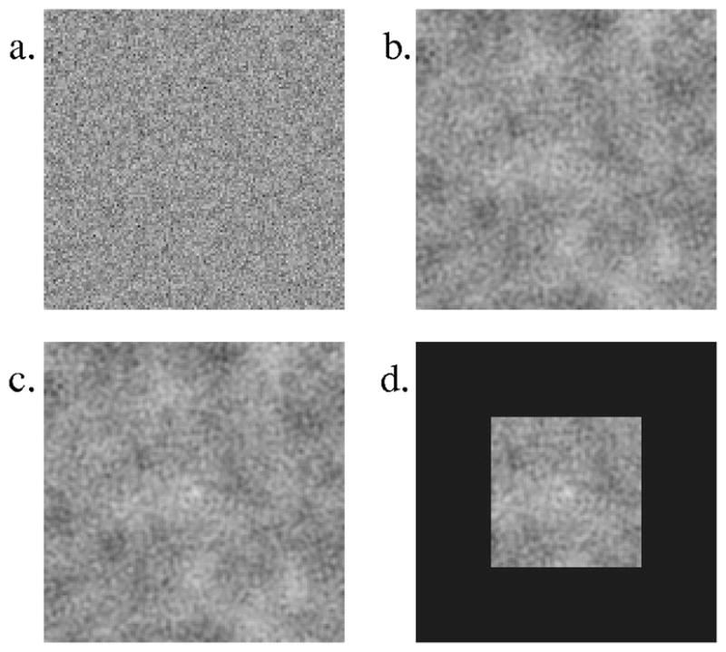
Four steps in the image-generation process: (a) initial white-noise field, (b) effect of filtering to induce pixel correlations, (c) effect with a signal added (with artificially high contrast for the purposes of visibility in this figure), (d) effect of cropping the edges to the final 64 × 64 pixels used in the psychophysical studies.

We will make extensive use of statistical properties of the images generated by the process just described—in particular, the image mean and covariance. For the purposes of specifying these quantities, it is convenient to describe an image as a one-dimensional column vector, indexed lexicographically by m = 0,…, M − 1. For an M_row × M_col image, M = M_row M_col. The image-generation procedure can then be defined as an affine transformation of the white-noise vector u (indexed as a 16,384-element column vector) to the final image f̂ (indexed as a 4,096-element column vector). The transformation is given by

$$\widehat{\mathbf{f}}=\mathbf{W}({\mathbf{F}}^{-1}\mathbf{\Lambda }\mathbf{Fu}+\mathbf{b}+{\delta }_{\text{SP}}\mathbf{s}),$$ (1)

where F is the matrix associated with the 2D-DFT, the diagonal matrix Λ implements the pointwise multiplication by the filter coefficients, the vector b is a mean background vector with all elements set to a constant value, and the vector s is the signal vector. The switch δ_SP is set to unity if the image is to be a signal-present image or zero if the image is to be a signal-absent image. The subregion extraction operation can be thought of as matrix multiplication with W, a rectangular matrix with 4,096 rows and 16,384 columns. Each row of W has a single nonzero element set to 1.0. The location of the nonzero element corresponds to the image pixel being extracted. The matrix transpose of W, indicated by W^t, can be thought of as the operation of padding as it embeds a subregion in a larger image.

The 2D-DFT matrix has an important orthogonality property that will be used often in this work. A unitary implementation of the 2D-DFT obeys the rule that¹⁴

$${\mathbf{F}}^{-1}={\mathbf{F}}^{†},$$ (2)

where the superscript † indicates the adjoint (transpose and complex conjugate) of the matrix. Nonunitary implementations of the 2D-DFT obey F⁻¹ = cF^† for some scaling constant c. For simplicity in the formulas that follow, we will assume that a unitary 2D-DFT is used.

B. Noise Correlation Structure

The components that influence the correlation structure of the images are implemented in the diagonal matrix Λ of Eq. (1). It is convenient to decompose Λ into three distinct components that represent the effects of quantum variability, anatomical variability, and regularization implemented during image reconstruction. These three components combine to define Λ as

$$\mathbf{\Lambda }\equiv \mathbf{B}{({\mathbf{N}}_q+{\mathbf{N}}_a)}^{1/2},$$ (3)

where N_q and N_a can be thought of as the NPS of the quantum noise and the anatomical variability, respectively, and B represents the effects of regularization. Each of the three terms on the right-hand side of Eq. (3) is itself a diagonal matrix. The exponent of 1/2 acting on N_q + N_a is interpreted in the usual sense for diagonal matrices as taking the positive square root of each diagonal element of the sum. As can be seen below, the diagonal elements of N_q and N_a are nonnegative, leading to real elements after the square root.

The diagonal elements of N_q, N_a, and B are specified in terms of the frequencies of the 2D-DFT. Each point of the 2D-DFT is associated with a lattice point in the 2D spatial-frequency domain. These lattice points form a square grid that is bounded by the Nyquist limit in each dimension. We will index points in the frequency domain by another lexicographic index k. The 2D frequency vector associated with element k is denoted by ρ_k. Since we will use radially symmetric (isotropic) functions in all of the studies reported here, it is most convenient to use the radial frequency ρ_k = ||ρ_k||..

Figure 2(a) plots the three components that make up Λ in terms of radial frequency. In the absence of any regularization and finite sampling effects,¹⁵ it is well established that quantum noise in tomographic reconstructions acquires a correlation structure well described by a ramp-like NPS.^5,6 Hence we model the diagonal elements of the quantum NPS by

Fig. 2.

Noise and signal power spectra. Plots of signal and noise power spectra as a function of radial frequencies (in pixels⁻¹). (a) Components of the noise-power spectrum (NPS). The total NPS is the sum of the quantum and anatomical components multiplied by the filter spectrum. (b) Components of the signal spectrum. The total signal spectrum is the product of the signal spectrum and the filter spectrum. Note that the signal power is plotted on a logarithmic scale to capture the low-amplitude peaks at 0.28 and 0.40 pixels⁻¹.

$${[{\mathbf{N}}_q]}_{kk}=\{\begin{array}{ll}{W}_q{\rho }_k\hfill & \text{if}{\rho }_k\ge {\rho }_q\hfill \\ W_q{\rho }_q\hfill & \text{if}{\rho }_k<{\rho }_q\hfill \end{array},$$ (4)

where ρ_q is set to the constant value 0.0078 pixel⁻¹ for all experiments and the magnitude W_q is varied in different experiments. The effect of this setting of ρ_q is to keep the dc component (ρ_k = 0) from going to zero. The resulting form of N_q is a ramp in radial frequency except very near the dc component, where the profile flattens. The value of the elements of N_q as a function of radial frequency are plotted (as the thin solid line) in Fig. 2(a). The change in the ramp spectrum near the origin is just visible at the lower left corner of the plot. Note that N_q should be thought of as a somewhat idealized quantity, since the actual contribution of the quantum noise to reconstructed images is influenced by a number of factors such as image system geometry, imperfect collimation, scattered radiation, and any regularization in the image reconstruction process.

Object—or patient-to-patient—variability results in another form of variability in reconstructed images. Like many natural images, anatomical variability often contains structures at varying scales with a resulting power spectrum that is approximated by an inverse-power law over a range of spatial frequencies.^16,17 In this work, object variability is modeled in terms of an anatomical NPS similar to that done in prior work by Rolland and Barrett¹⁸ and by Burgess.¹⁹ Diagonal elements of the anatomical NPS are given by

$${[{\mathbf{N}}_a]}_{kk}=\frac{W_a}{1+{({\rho }_k/{\rho }_a)}^{\beta }},$$ (5)

where ρ_a is a constant set to 0.0156 that determines the frequencies where the inverse-power law holds. For values of ρ_k that are large relative to ρ_a, the anatomical NPS is very nearly proportional to ${\rho }_k^{-\beta }$. For small values of ρ_k, the anatomical NPS departs from a power-law form and remains bounded. The setting of ρ_a used here results in spatial correlations that follow the inverse-power-law NPS until correlation lengths are on the order of 64 pixels. The exponent β controls the rate of falloff of the power spectrum. This parameter has been used to quantify the complexity of anatomical variability, with values of 3.0–4.0 reported in mammography,^9–12 3.4 in coronary angiography,¹¹ and 3.7–3.9 in single-photon emission computed tomography liver scans.⁷ Values of β used in the psychophysical studies vary from β = 2.0 to β = 4.0. For the component of the anatomical NPS in Fig. 2(a), β = 4.0. The parameter W_a controls the magnitude of the anatomical fluctuations in the images. Like the quantum NPS, the actual contribution of anatomical variability to the reconstructed images is influenced by regularization. However, the effect of regularization is less severe on the model of anatomical variability used here, since the areas of highest variability in N_a occur at low spatial frequencies, where there is little regularization.

Regularization is an integral part of most image-reconstruction algorithms, since unregularized reconstructions demonstrate considerable noise amplification. There are a number of ways to implement regularization for image reconstruction in the form of constraints, prior distributions, sieves, iterative stopping criteria, and smoothing filters. Smoothing filters are particularly well suited to the present work because the filter can be directly implemented in the image-generation process as part of Λ in Eq. (3). The frequency profile of the regularizing filter used here is in the form of a Butterworth filter:

$${[\mathbf{B}]}_{kk}=\frac{1}{1+{({\rho }_k/{\rho }_c)}^{2\nu }}.$$ (6)

The cutoff point of the filter, denoted by the parameter ρ_c, is the radial frequency at which the value of the filter is 1/2. The parameter ν is on the order of the Butter-worth filter. This component determines how fast the filter falls off near the cutoff point. For all experiments, the order of the Butterworth filter is fixed at a value of ν = 4.

C. Signal Profile

The signal profile in reconstructed images includes the effects of regularization in the reconstruction algorithm; the signal-present profile can be thought of as an unregularized profile s₀ that is filtered with a transfer function of the regularizing filter implemented by the matrix B found in Eq. (3). Each element of the unregularized signal vector, denoted by s₀, is defined in the spatial domain by

$${[{\mathbf{s}}_0]}_m=\{\begin{array}{ll}{A}_s{\left[1-{\left(\frac{\left|\right|{\mathbf{r}}_m-{\mathbf{r}}_c\left|\right|}{R}\right)}^2\right]}^n\hfill & \text{if}\left|\right|{\mathbf{r}}_m-{\mathbf{r}}_c\left|\right|\le R\hfill \\ 0\hfill & \text{otherwise}\hfill \end{array},$$ (7)

where ||r_m − r_c|| is the distance between the location of the mth image pixel (r_m) and the signal center (r_c). The signal contrast is controlled by A_s, the signal amplitude is in gray levels, and R is the signal radius in pixel units. The exponent n determines the rate at which the signal profile goes to zero near the edge. For all the experiments, R is set to 4.0, and n is set to 1.5. This functional form has been used by Burgess et al.²⁰ to fit the profile of nodule data collected by Samei et al.²¹

Applying the regularizing filter to s₀ yields the filtered signal profile

$$\mathbf{s}={\mathbf{F}}^{†}\mathbf{BF}{\mathbf{s}}_0.$$ (8)

The spectrum of the signal before and after regularization by B is plotted as a function of radial frequency in Fig. 2(b). The amplitude of the spectra in this figure is plotted on a logarithmic scale so that the small peak in the spectrum near 0.25 pixel⁻¹ is clearly visible. This scaling also shows the relatively small effects of the regularizing filter on the signal for this particular cutoff point (ρ_c = 0.3). Significant differences in the spectrum are not apparent until the amplitude has fallen off by nearly 3 orders of magnitude.

D. Image Statistics

The statistical properties of interest for this work are the image mean and the image covariance of signal-absent and signal-present images generated by the process described in Subsection 2.A. These quantities can be determined directly from the image-generating process given in Eq. (1) provided that we know the mean and the covariance of the white-noise vector u and the effect of an affine transformation on these quantities.

The mean of a random vector x is another vector μ_x = 〈x〉, where the angle brackets indicate the mathematical expectation of the random quantity inside. The covariance matrix for x is defined by the matrix-valued expectation K_x = 〈(x − μ_x)(x − μ_x)⁺〉. For an affine transformation of x, given by

$$\mathbf{y}=\mathbf{Ax}+\mathbf{c},$$ (9)

where the matrix A and the vector c are assumed to be nonrandom quantities, the mean and the covariance are defined by

$${\mathit{\mu }}_{\mathbf{y}}=\mathbf{A}{\mathit{\mu }}_{\mathbf{x}}+\mathbf{c},{\mathbf{K}}_{\mathbf{y}}=\mathbf{A}{\mathbf{K}}_{\mathbf{x}}{\mathbf{A}}^{†},$$

respectively.²²

The starting point for the image-generation procedure is the white-noise vector u. Since each element of u is independent, has zero mean, and has unit variance, the mean of u is μ_u = 0 and the covariance matrix is the identity matrix K_u = I. For the transformation from u to f̂ in Eq. (1), we see that the components of Eq. (9) are given by A = WF^†ΛF and c = W(b + δ_SPs). Hence the mean vector is given by

$${\mathit{\mu }}_{\widehat{\mathbf{f}}}=\mathbf{W}(\mathbf{b}+{\delta }_{\text{SP}}\mathbf{s}),$$

and the covariance matrix is given by

$$\begin{array}{l}{\mathbf{K}}_{\widehat{\mathbf{f}}}=\mathbf{W}{\mathbf{F}}^{†}\mathbf{\Lambda }\mathbf{F}{\mathbf{K}}_{\mathbf{u}}{(\mathbf{W}{\mathbf{F}}^{†}\mathbf{\Lambda }\mathbf{F})}^{†}\\ =\mathbf{W}{\mathbf{F}}^{†}{\mathbf{\Lambda }}^2\mathbf{F}{\mathbf{W}}^{\text{t}}.\end{array}$$ (10)

The covariance does not depend on the value of the signal switch δ_SP. Hence the covariance matrices associated with signal-present and signal-absent classes of images are both equivalent to K_f̂. The mean image μ_f̂ is dependent on the value of δ_SP, and hence the mean signal-present image μ_f̂|sp is different from the mean signal-absent image μ_f̂|sa. We will denote the mean difference between signal-present and signal-absent images by Δμ_f̂, defined as

$$\begin{array}{l}\mathrm{\Delta }{\mathit{\mu }}_{\widehat{\mathbf{f}}}\equiv {\mathit{\mu }}_{\widehat{\mathbf{f}}\mid \text{sp}}-{\mathit{\mu }}_{\widehat{\mathbf{f}}\mid \text{sa}}\\ =\mathbf{W}(\mathbf{b}+\mathbf{s})-\mathbf{Wb}\\ =\mathbf{Ws}.\end{array}$$ (11)

If we replace s and Λ by their definitions in Eqs. (8) and (3), respectively, we obtain formulas for the statistical properties of interest in this work in terms of the modeled components of the imaging chain described in the previous section. For the mean image difference, we have

$$\mathrm{\Delta }{\mathit{\mu }}_{\widehat{\mathbf{f}}}=\mathbf{W}{\mathbf{F}}^{†}\mathbf{BF}{\mathbf{s}}_0,$$ (12)

and for the image covariance we have

$${\mathbf{K}}_{\widehat{\mathbf{f}}}=\mathbf{W}{\mathbf{F}}^{†}{\mathbf{B}}^2({\mathbf{N}}_q+{\mathbf{N}}_a)\mathbf{F}{\mathbf{W}}^{\text{t}}.$$ (13)

3. EVALUATION OF DETECTION PERFORMANCE

Section 2 described a method for generating images and derived some relevant statistical properties of those images. The motivation for deriving these quantities is to understand how they influence the performance of detection tasks. In this section, we describe how the images and the statistical properties are used to assess performance in the context of two-alternative forced-choice (2AFC) detection.

A. Image Response Variables

In each trial of a 2AFC detection task, two images are presented to the observer. One image contains a signal [in the context of this work, generated by Eq. (1) with δ_SP = 1], and the other does not contain a signal [generated by Eq. (1) with δ_SP = 0]. The observer performs the task by identifying the image that to a greater degree appears to contain the signal in each trial. This process is repeated over many trials. This section describes a general model of how an observer arrives at a decision when presented with two images in a 2AFC trial.

Throughout this work, we will utilize models of the detection process that act directly on an image vector f̂ rather than on the intensity of the displayed image. The rationale behind this simplification is that the parameters of the images, not the display device, are the subject of interest. However, the human observer can access reconstructed images only after display. Hence the validity of this simplifying step in attempts to model the human observer requires that display of the images not significantly affect task performance. This seems to be a valid assumption in noise-limited tasks of the sort considered here, where the absence of image noise would render the signal visually obvious to the observer. For example, Judy and Swensson^23,24 and Judy et al.²⁵ have found little dependence over a broad range of display parameters for detection in computed tomography images. Image display is likely to have a much greater impact on task performance when the signal contrast is near the threshold for visual detection.

We begin with the generation of a response variable by an observer that acts on f̂. This process yields an observer-response variable λ, defined by

$$\lambda =w(\widehat{\mathbf{f}})+\epsilon .$$ (14)

The function w(f̂) is the response to the image data, while ε represents the internal noise in the observer response that results in a noisy—or randomized—decision maker. Internal noise is an important component for describing human-observer performance, since it is demonstrably present in decisions made by human observers.^26–28 We assume that ε is a zero-mean random variable. Furthermore, the observer internal noise is generally assumed to be uncorrelated with the image.

The model for the process by which an observer makes a decision in a 2AFC trial is as follows. Let us denote the outcome of the ith trial as the random variable o_i. When a correct decision is made, o_i = 1, and when an incorrect decision is made, o_i = 0. The model of detection performance assumes that the observer forms a response to both images according to Eq. (14) and chooses the image with the larger response. We denote the response in the ith trial to the signal-present image as ${\lambda }_i^{+}$ and the response to the signal-absent image as ${\lambda }_i^{-}$; then the decision can be described by

$$o_i=\{\begin{array}{ll}0\hfill & \text{if}{\lambda }_i^{+}-{\lambda }_i^{-}<0\hfill \\ 1\hfill & \text{if}{\lambda }_i^{+}-{\lambda }_i^{-}>0\hfill \end{array}.$$ (15)

We are assuming continuous probability densities on ${\lambda }_i^{+}$ and ${\lambda }_i^{-}$, and hence the probability of observing an equivocal decision ( ${\lambda }_i^{+}-{\lambda }_i^{-}=0$) is zero.

The concept of a model observer is often used in this work and in the literature.^29,30 The term is used to describe a decision strategy based on an observer response generated by a mathematical model. In other words, if we specify a particular functional form for w(f̂) in Eq. (14) and a probability distribution on ε, then we have defined a model observer.

B. Measures of Performance

A measure of detection performance is a formal way to quantify how well a given detection strategy performs a task. The most fundamental measure of performance in a forced-choice task is the proportion correct, defined as the expected value of o_i in Eq. (15) and denoted by P_C. For a 2AFC experiment P_C can be interpreted either as the probability of reaching a correct decision in each trial of a forced-choice experiment or as the probability that ${\lambda }_i^{+}$ is greater than ${\lambda }_i^{-}$. This latter interpretation can be used to show that P_C is equivalent to the area under the receiver operating characteristic curve.³¹ Thus P_C has an interpretation beyond the forced-choice detection task.

A second measure of performance, the observer signal-to-noise ratio (SNR), is given in terms of the mean and the variance of the ${\lambda }_i^{+}$ and ${\lambda }_i^{-}$ variables.^32,33 It is defined as

$${\text{SNR}}_w^2=\frac{{({\mu }_{{\lambda }^{+}}-{\mu }_{{\lambda }^{-}})}^2}{\frac{1}{2}({\sigma }_{{\lambda }^{+}}^2+{\sigma }_{{\lambda }^{-}}^2)},$$ (16)

where μ_λ⁺ and ${\sigma }_{{\lambda }^{+}}^2$ are the mean and the variance of ${\lambda }_i^{+}$ and μ_λ⁻ and ${\sigma }_{{\lambda }^{-}}^2$ are the mean and the variance of ${\lambda }_i^{-}$. The subscript on the observer SNR is included to emphasize the dependence of this quantity on w, the observer response function in Eq. (14).

A third measure of performance, which we refer to as the detectability and denote by d_A, provides the link between P_C and the observer SNR. The detectability is defined simply as the transformation of P_C given by

$$d_A=\sqrt{2}{\mathrm{\Phi }}^{-1}(P_C),$$ (17)

where Φ⁻¹ is the inverse cumulative normal distribution. It has been shown (see, for example, Barrett et al.³³) that if ${\lambda }_i^{+}$ and ${\lambda }_i^{-}$ are independent and Gaussian distributed, then SNR_w = d_A. In this case, the observer SNR is equivalent to the observer detectability.

C. Liner Model Observers

A linear model observer is defined as a special case of Eq. (14) in which the response function w is linear in its argument. In this case, the observer response can be specified in terms of an inner product with a vector of weights w that has the same dimension as that of the image vector. The vector of weights is often referred to as the observer template. The resulting form of Eq. (14) is given by

$$\lambda ={\mathbf{w}}^{\text{t}}\widehat{\mathbf{f}}+\epsilon .$$ (18)

As mentioned above, we must specify a distribution on the internal-noise component to fully identify a model observer. We will take ε to be a Gaussian random variable, independent of f̂, with a mean value of zero and variance ${\sigma }_{\epsilon }^2$. Various choices for the internal-noise variance are used, including ${\sigma }_{\epsilon }^2=0$, which results in a noiseless (non-randomized) decision maker. It should be noted that the use of a single internal-noise variable—ε in this case—does not necessarily imply a single source of internal noise. The ε term should be thought of as a composite of internal noise from various sources.

The combination of a linear observer response function and Gaussian-distributed internal noise allows us to write the mean and the variance of ${\lambda }_i^{+}$ and ${\lambda }_i^{-}$ in terms of the statistical properties of f̂ and ε. Using the rules of linear transformation of Gaussian random variables, it is straightforward to derive that

$$\begin{array}{l}{\mu }_{{\lambda }^{+}}-{\mu }_{{\lambda }^{-}}={\mathbf{w}}^{\text{t}}\mathrm{\Delta }{\mathit{\mu }}_{\widehat{\mathbf{f}}},\\ {\sigma }_{{\lambda }^{+}}^2={\sigma }_{{\lambda }^{-}}^2={\mathbf{w}}^{\text{t}}{\mathbf{K}}_{\widehat{\mathbf{f}}}\mathbf{w}+{\sigma }_{\epsilon }^2,\end{array}$$

where Δμ_f̂ is the mean difference in signal-present and signal-absent images given in Eq. (11) and K_f̂ is the common image covariance given in Eq. (10). With these two relations, we can write the observer SNR in terms of the model observer and the statistical properties of the images as

$${\text{SNR}}_{\mathbf{w}}^2=\frac{{({\mathbf{w}}^{\text{t}}\mathrm{\Delta }{\mathit{\mu }}_{\widehat{\mathbf{f}}})}^2}{{\mathbf{w}}^{\text{t}}{\mathbf{K}}_{\widehat{\mathbf{f}}}\mathbf{w}+{\sigma }_{\epsilon }^2}.$$ (19)

For multivariate Gaussian-distributed images and a Gaussian-distributed internal-noise component, the resulting observer-response variable will also be a Gaussian. Hence the observer SNR given in Eq. (19) is equivalent to the observer detectability defined in Eq. (17).

D. Psychophysical Experiments

The results of this work are centered on human-observer performance as measured from psychophysical studies. For human observers in a 2AFC task, we do not have access to the observer response variables ${\lambda }_i^{+}$ and ${\lambda }_i^{-}$. The only observable outcome of a given trial is o_i, the binary variable indicating a correct or incorrect decision.

While the lack of access to the observer-response variables precludes direct calculation of an observer SNR, it does not stop us from estimating other measures of performance. In particular, the proportion correct can be estimated by taking the sample average of the o_i variables.³¹ If N_trial is the total number of trials in an experiment, then the estimate of P_C is given by

$${\widehat{P}}_C=\frac{1}{N_{\text{trial}}}\sum _{i=1}^{N_{\text{trial}}}{o}_i.$$ (20)

From the estimate of proportion correct, we can obtain an estimate of the observer detectability by applying the transform in Eq. (17) to get

$${\widehat{d}}_A=\sqrt{2}{\mathrm{\Phi }}^{-1}({\widehat{P}}_C).$$ (21)

Most of the results reported in this work contain comparisons of human-observer detectability, estimated by Eq. (21), with the observer SNR for a variety of model observers computed from Eq. (19). We emphasize that this is a fair comparison (under the assumption that image display is not a significant factor), since the observer SNR for linear observers is equivalent to detectability for the images considered. The main difference between the two measures of performance is that the human-observer detectability is an estimate, while model-observer SNR is computed analytically from the mean and the covariance of the image-generation process.

There are a number of practical considerations in design and environment of psychophysical experiments. We postpone discussion of these issues until Section 5.

4. MODEL OBSERVERS

This section describes a number of different linear model observers in terms of their observer templates, as defined in Eq. (18). We begin with three nonprewhitening observers that are generally easy to implement. We refer to these observers as nonprewhitening because they make no attempt to decorrelate, or “whiten,” the noise in the images. Practically, this restriction means that the observer template is independent of the image covariance matrix. The next observer considered is the Hotelling observer. Because of the Gaussian process for generating the data (with equal covariances in both signal-present and signal-absent images), the Hotelling observer is also the optimal detection strategy and hence the ideal observer for this task. Finally, we describe a family of model observers, called channelized-Hotelling observers. Proposed by Myers³⁴ and Myers and Barrett,³⁵ these observers combine elements of the human visual system (i.e., channels) with a Hotelling-type decision strategy to perform the detection task.

A. Nonprewhitening Observers

The simplest of the nonprewhitening observers is a region-of-interest (ROI) observer. As the name implies, this observer is specified by the spatial extent of a ROI. The ROI upon which the observer is based is defined as a collection of adjacent pixels in the image. In this case, the ROI-observer template is given by

$${[{\mathbf{w}}_{\text{ROI}}]}_m=\{\begin{array}{ll}1\hfill & \text{if}{\mathbf{r}}_m\in \text{ROI}\hfill \\ 0\hfill & \text{if}{\mathbf{r}}_m\notin \text{ROI}\hfill \end{array},$$ (22)

where r_m is the spatial location of the mth pixel. For this work, the ROI is defined to be the spatial extent of the signal, a circle of radius 4.0 pixels about the middle pixel. In the case of white noise and a signal profile that attains a single value within the region of interest, this observer profile is optimal and forms the basis for the Rose model.³⁶

In more realistic imaging situations, the ROI observer is markedly suboptimal and has a very limited capacity to adapt to the image characteristics. The observer is unaffected by the image covariance and utilizes only rudimentary information about the signal profile. Any two signal profiles with the same spatial extent result in the same observer template.

The nonprewhitening-matched-filter (NPW) observer is defined as the output of a matched filter that is tuned (or adapted) to the signal profile. The observer template associated with this model observer is given by

$${\mathbf{w}}_{\text{NPW}}=\mathrm{\Delta }{\mathit{\mu }}_{\widehat{\mathbf{f}}}.$$ (23)

Unlike the ROI observer, the NPW observer makes full use of the signal profile, and hence the observer can be thought of as fully adaptable to the signal. This observer was considered a good candidate as a model of human observers in a number of early works that considered white noise and noise with a high-pass correlation structure.^{23,24,34,37–42} In a later study with low-pass correlated noise, Rolland and Barrett¹⁸ found that humans significantly outperformed the NPW observer.

Burgess¹⁹ has proposed a modification to the NPW observer by composing it with a convolution filter representing the effects of contrast sensitivity in the human visual system. This convolution filter is commonly referred to as the eye filter. The eye filter is specified in the spatial-frequency domain by a radially symmetric transfer function with profile given by Barten.⁴³ The functional form of the eye filter transfer function is

$$E(\rho )={\rho }^{\eta }exp(-c{\rho }^2),$$ (24)

where the parameter c was set so that the maximum value of E(ρ) occurs at the peak of the human contrast-sensitivity function at approximately 4.0 cycles per degree visual angle. Burgess found that η = 1.3 best fit human-observer data.

We will follow Burgess’s notation and denote the eye-filtered NPW observer by the acronym NPWE. The observer template associated with this observer is given by

$${\mathbf{w}}_{\text{NPWE}}={\mathbf{E}}^{\text{t}}\mathbf{E}\mathrm{\Delta }{\mathit{\mu }}_{\widehat{\mathbf{f}}},$$ (25)

where the matrix E implements the effects of the eye filter. For a discrete image vector, E is defined by

$$\mathbf{E}={\mathbf{F}}^{†}{\mathbf{\Lambda }}_{\text{eye}}\mathbf{F},$$

where F is the DFT matrix and Λ_eye is a diagonal matrix with the diagonal elements given by

$${[{\mathbf{\Lambda }}_{\text{eye}}]}_{kk}=E({\rho }_k).$$ (26)

Note that the eye filter appears twice in Eq. (25) because the observer is implemented by computing a scalar product between the eye-filtered image Ef̂ and the eye-filtered difference-signal profile EΔμ_f̂. The resulting scalar product is

$${(\mathbf{E}\mathrm{\Delta }{\mathit{\mu }}_{\widehat{\mathbf{f}}})}^{\text{t}}\mathbf{E}\widehat{\mathbf{f}}=\mathrm{\Delta }{\mathit{\mu }}_{\widehat{\mathbf{f}}}^{\text{t}}{\mathbf{E}}^{\text{t}}\mathbf{E}\widehat{\mathbf{f}}={\mathbf{w}}_{\text{NPWE}}^{\text{t}}\widehat{\mathbf{f}}.$$

B. Hotelling Observer

Unlike the NPW observers, the Hotelling observer utilizes information about spatial correlations in its observer template. The observer template is given by⁴⁴

$${\mathbf{w}}_{\text{HOT}}={\mathbf{K}}_{\widehat{\mathbf{f}}}^{-1}\mathrm{\Delta }{\mathit{\mu }}_{\widehat{\mathbf{f}}}.$$ (27)

The inverse-covariance matrix serves both to decorrelate—or whiten—the noise in the image and to match the mean signal profile to one that has passed through the whitening process. When the covariance matrix is stationary, the Hotelling-observer template is the equivalent of a prewhitening matched filter. This observer template is optimal in the sense that it maximizes the linear observer SNR in Eq. (19) in the absence of internal noise. In this case, the maximal observer SNR is given by

$${\text{SNR}}_{{\mathbf{w}}_{\text{HOT}}}={(\mathrm{\Delta }{\mathit{\mu }}_{\widehat{\mathbf{f}}}{\mathbf{K}}_{\widehat{\mathbf{f}}}^{-1}\mathrm{\Delta }{\mathit{\mu }}_{\widehat{\mathbf{f}}})}^{1/2}.$$ (28)

For images with a multivariate Gaussian distribution and the same correlation structure in both signal-absent and signal-present images, the Hotelling observer is equivalent to the ideal observer.³³

Note that the observer template given in Eq. (27) is sensitive to both the mean signal and the image covariance. If either of these components changes, then the resulting strategy for performing the task is altered. Therefore the Hotelling observer can be thought of as adapting to both the signal profile and the image covariance. This point is of interest because there has been a considerable effort to understand the degree to which human observers are able to adapt to the statistical properties of images.^13,18,29 The Hotelling observer relates optimal adaptation to the ability to invert the image covariance matrix, which is in turn related to the notion of decorrelating, or prewhitening, the noise.

Practical implementation of the Hotelling observer can be difficult because of problems inverting K_f̂. Computation of the inverse covariance by numerical inversion can be extremely time consuming because of the large size of the matrix as well as subject to severe numerical error if the covariance matrix is ill conditioned. The problem of ill conditioning will also confound iterative methods for computing inverse-covariance products with slow convergence.

For the results reported in this work, the Hotelling-observer performance is evaluated ignoring the image extraction step described in Subsection 2.A. This allows us to work with a filtered-noise field that is decorrelated by the DFT. As a result, the inverse covariance is easily computed from the NPS. With the use of this approximation, the SNR of the Hotelling observer is given by

$${\text{SNR}}_{{\mathbf{w}}_{\text{HOT}}}\simeq {({\mathbf{s}}_{\text{filt}}^{\text{t}}{\mathbf{K}}_{{\mathbf{u}}_{\text{filt}}}^{-1}{\mathbf{s}}_{\text{filt}})}^{1/2}={[{\mathbf{s}}^{\text{t}}{\mathbf{F}}^{†}{({\mathbf{N}}_q+{\mathbf{N}}_a)}^{-1}\mathbf{Fs}]}^{1/2}.$$ (29)

Note that the effects of the Butterworth filter are absent from the Hotelling-observer SNR. Because the filter is present in both the mean signal profile and the noise covariance, it cancels out of Eq. (29).

C. Channelized-Hotelling Observers

The notion of channels in the human visual system has been studied intensively in vision science for many years.^45–47 The application of channelized observers to medical image-quality assessment began with the work of Myers³⁴ and Myers and Barrett,³⁵ who introduced the channelized Hotelling observer. A detailed development of this observer can be found in that work or more recently in work by Abbey⁴⁸ and Abbey and Bochud.⁴⁹ For the purposes of this paper, we provide an abbreviated description.

A channelized Hotelling observer performs a detection task after first reducing the image to a smaller (usually much smaller) set of channel response variables. The channel response variables are defined by the transformation

$$\mathbf{u}={\mathbf{T}}^{\text{t}}\widehat{\mathbf{f}}+\mathit{\epsilon },$$ (30)

where the column vectors of the matrix T each represent the spatial profile of a channel and the vector ε contains the internal noise in each channel. The internal noise in the channels is presumed to be zero mean, and it has a covariance matrix denoted by K_ε. If we postulate that the channel responses are transformed into a scalar observer-response variable by a Hotelling strategy, then the observer template (in the image domain) is given by

$${\mathbf{w}}_{\text{CH}}=\mathbf{T}{({\mathbf{T}}^{\text{t}}{\mathbf{K}}_{\widehat{\mathbf{f}}}\mathbf{T}+{\mathbf{K}}_{\epsilon })}^{-1}{\mathbf{T}}^{\text{t}}\mathrm{\Delta }{\mathit{\mu }}_{\stackrel{\sim }{\mathbf{f}}}.$$ (31)

The variance of the internal noise in the observer response is given by

$${\sigma }_{int}^2=\mathrm{\Delta }{\mathit{\mu }}_{\widehat{\mathbf{f}}}^{\text{t}}\mathbf{T}{({\mathbf{T}}^{\text{t}}{\mathbf{K}}_{\widehat{\mathbf{f}}}\mathbf{T}+{\mathbf{K}}_{\epsilon })}^{-1}{\mathbf{K}}_{\epsilon }{({\mathbf{T}}^{\text{t}}{\mathbf{K}}_{\widehat{\mathbf{f}}}\mathbf{T}+{\mathbf{K}}_{\epsilon })}^{-1}{\mathbf{T}}^{\text{t}}\mathrm{\Delta }{\mathit{\mu }}_{\widehat{\mathbf{f}}}.$$ (32)

If we substitute in, according to Eqs. (31) and (32), the formula for observer SNR given in Eq. (19), we obtain

$${\text{SNR}}_{{\mathbf{w}}_{\text{CH}}}={[\mathrm{\Delta }{\mathit{\mu }}_{\widehat{\mathbf{f}}}^{\text{t}}\mathbf{T}{({\mathbf{T}}^{\text{t}}{\mathbf{K}}_{\widehat{\mathbf{f}}}\mathbf{T}+{\mathbf{K}}_{\epsilon })}^{-1}{\mathbf{T}}^{\text{t}}\mathrm{\Delta }{\mathit{\mu }}_{\widehat{\mathbf{f}}}]}^{1/2}.$$ (33)

The channel filters also provide a mechanism for partial adaptation to the signal profile and the noise structure. The channelized Hotelling observer can adapt to the signal profile and the image covariance only after they have passed through T. Hence this observer will adapt to a different covariance only if it causes a change in T^tK_f̂T. By the same argument, this observer is sensitive only to changes in the signal profile that cause a change in T^tΔμ_f̂. For sparse channel models with just a few channels, a significant loss of information may occur in the formation of the channel responses. This loss of information combined with any internal noise in the channel responses translates into suboptimal performance.

A useful practical point is that the channelized-Hotelling observer can avoid some computational difficulties in evaluating the Hotelling observer. Because of the transformation by T, the dimension of the necessary inverse is generally reduced to the dimension of the relatively small number of channel responses. This reduction in dimension is usually substantial enough that the inverse of the channel covariance matrix T^tK_f̂T + K_ε can be obtained directly by numerical inversion. Note also that T^tK_f̂T + K_ε is guaranteed to be invertible if K_ε is nonsingular, regardless of the rank of K_f̂. Hence the combination of channels and the internal noise associated with them can actually make evaluation of the observer easier and more stable from a computational point of view.⁵⁰

We now describe three channel models used to evaluate the channelized-Hotelling observer for the experiments described in Section 5.

D. Channel Profiles

Equation (30) casts the formation of each channel response as an inner product between the image vector and a column of the filter bank T. Most of the literature describes visual channels in terms of the Fourier transform of a retinal image. If we define the jth channel profile in the coordinate system of the displayed image, we obtain a channel profile C_j(ρ), which is a function of the two-dimensional spatial-frequency variable ρ. The spatial sensitivity function associated with this channel profile is t_j(r), the inverse Fourier transform of C_j(ρ). We implement the channels in the discrete image domain by using the inverse DFT to define the jth column of T by

$${\mathbf{t}}_j={\mathbf{F}}^{†}{\mathbf{c}}_j,$$

where

$${[{\mathbf{c}}_j]}_k=C_j({\mathit{\rho }}_k).$$

The first implementations of the channelized-Hotelling observer^34,35 utilized radially symmetric channel filters with a square bandpass profile in radial frequency. The justification for the radial symmetry was that the signal profile and the noise covariance for these experiments were also radially symmetric. Therefore radially symmetric channels resulted in a large economy in the number of channels needed to cover a range of spatial frequencies. These justifications apply equally well to the present work. Both the signal profile and the covariance structure of the noise are defined in terms of radially symmetric functions. Hence we use radially symmetric channel profiles in this work as well.

In the radial frequency domain, the square filters used by Myers are defined by a starting frequency ρ₀. This frequency serves as the starting point of the first channel. The upper frequency of this channel is defined to be ρ₁ = αρ₀ with α > 1. The starting frequency of the second channel is set to the upper frequency of the first. The upper frequency of the second channel is then given by ρ₂ = αρ₁. This system for defining the channel filters is continued for the remaining channels. The radial frequency profile of the jth channel is given by

$$C_j(\rho )=\{\begin{array}{ll}0\hfill & \text{for}\rho \le {\rho }_0{\alpha }^{j-1}\hfill \\ 1\hfill & \text{for}{\rho }_0{\alpha }^{j-1}<\rho \le {\rho }_0{\alpha }^j\hfill \\ 0\hfill & \text{for}\rho >{\rho }_0{\alpha }^j\hfill \end{array}$$ (34)

The square-channel model used in Section 5 (denoted SQR) has a total of four channels, a starting frequency of ρ₀ = 0.015, and α set to 2.0. The profiles for this channel model are plotted in Fig. 3A.

Fig. 3.

Channel profiles for channelized-Hotelling observers. The three plots illustrate the frequency response for the square (SQR), sparse difference-of-Gaussians (S-DOG), and dense difference-of-Gaussians (D-DOG) channel models used in this work.

A second radially symmetric model has been utilized more recently^51,52 that incorporates overlapping difference-of-Gaussians (DOG) functions for the channel sensitivity functions. DOG functions are one of several bandpass profiles that have long been used to model spatial-frequency selectivity in the human visual system.^53,54 With this model, the radial frequency profile of the jth channel is given by

$$C_j(\rho )=exp\left[-\frac{1}{2}{\left(\frac{\rho }{Q{\sigma }_j}\right)}^2\right]-exp\left[-\frac{1}{2}{\left(\frac{\rho }{{\sigma }_j}\right)}^2\right].$$ (35)

The standard deviation of each channel, σ_j, is chosen in an analogous fashion to the frequencies of the square-channel model. From an initial σ₀, each of the σ_j values in Eq. (35) is defined by σ_j = σ₀α^j. The multiplicative factor Q > 1 defines the bandwidth of the channel. Two DOG channel models are used in this work. The first is a sparse model (denoted by S-DOG) that uses three channels. The channel parameters for this model are σ₀ = 0.015, α = 2.0, and Q = 2.0. The channel profiles of the S-DOG model are given in Fig. 3B. A second dense set of DOG channels (denoted by D-DOG) is investigated as well. This channel model uses ten channels with channel parameters of σ₀ = 0.005, α = 1.4, and Q = 1.67. The channel profiles of the D-DOG model are plotted in Fig. 3C.

More involved channel models that use channel profiles tuned to specific angular orientations and phase factors have been proposed by Watson⁵⁵ and Daly.⁵⁶ Eckstein and Whiting⁵⁷ have been successful in predicting human performance in patient-structured noise by using an implementation of the Watson model. Burgess et al.¹³ have reported results by using channels defined from Daly’s model. Practical implementations of these models typically involve many more channel responses.

5. RESULTS

In this section, we report the results of a number of psychophysical studies using images generated by the procedure described in Section 2. Human-observer performance, reported in terms of the detectability defined in Eq. (21), is compared with ensemble calculations of model-observer SNR obtained from Eq. (19) by using the statistical properties of the images described in Section 2.

A. Rationale and Description of Experiments

The large number of parameters in the definitions of the signal profile and the NPS leave many possibilities for variables to study. Of these, we have considered three specific effects here for their relevance to topics in imaging.

1. Regularization Study

The regularization study is most germane to the subject of image-reconstruction algorithms, since most algorithms have one or more parameters that allow the user to control the level of regularization implemented in the final reconstructed image. The regularization generally results in suppression of higher spatial frequencies in much the same way that the Butterworth filter in Subsection 2.A modulates the signal and noise spectra. The study presented in this section quantifies the effect of the frequency cutoff of the Butterworth filter, ρ_c, on detection performance. Values of this parameter range from 0.450 to 0.060 cycle/pixel.

The parameter of interest in the seven experiments that constitute this study is ρ_c, the cutoff frequency of the Butterworth filter given in Eq. (6). The value of ρ_c ranges from a value of ρ_c = 0.06, which produced very smooth, highly regularized images, to a value of ρ_c = 0.45, which produced images with little regularization at all. Table 1 lists the relevant parameters of each experiment in the study. The images in each experiment were scaled so that the pixel standard deviation was approximately 20.0 gray levels across all experiments, and hence A_s, W_a, and W_q vary relative to each other in the different experiments. The exponent β of the anatomical NPS was fixed at 3.0 for all experiments in this first study.

Table 1.

Parameter Settings for the Regularization Study^a

Exp. No.	As	Wa	Wq	ρc
1	25.7	80021.	1724.9	0.450
2	33.3	134166.	2894.7	0.323
3	38.9	184259.	3975.3	0.230
4	42.3	216412.	4665.4	0.165
5	44.4	238594.	5145.4	0.117
6	46.2	258503.	5578.6	0.084
7	48.5	284949.	6145.3	0.060

^aThe parameter A_s refers to the signal amplitude (prior to the Butterworth filter), W_a refers to the magnitude of the anatomical NPS, W_q refers to the magnitude of the quantum NPS, and ρ_c refers to the cutoff frequency of the regularizing (Butterworth) filter.

Table 1 summarizes the relevant parameters of each experiment in this study. The amplitudes of the quantum NPS and the anatomical NPS are proportional to each other and scaled so that the noise amplitude (the pixel standard deviation) remains constant across all conditions. The signal amplitude has been set in proportion to the square root of the NPS amplitudes. With these settings, ideal-observer SNR is constant across experimental conditions. A sample image from experiments 1, 4, and 7 is shown in Fig. 4.

Fig. 4.

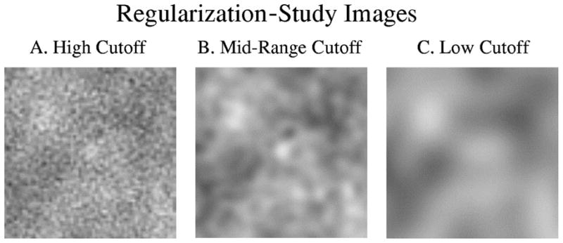
Sample images used in the regularization study experiments. The successive smoothing of the image reflects the effect of a lower cutoff frequency. A. High-frequency cutoff in the regularizing filter (experiment 1: ρ_c = 0.450). B. Midrange frequency cutoff in the regularizing filter (experiment 4: ρ_c = 0.165). C. Low-frequency cutoff in the regularizing filter (experiment 7: ρ_c = 0.060).

2. Exposure-Time Study

The parameter of interest in the exposure-time study is the ratio of W_a, the magnitude of the anatomical NPS in Eq. (5), to W_q, the magnitude of the quantum noise NPS in Eq. (4). In the context of emission imaging, Rolland and Barrett¹⁸ explicitly derive the exposure-time dependence of both the anatomical and quantum NPS’s of unreconstructed data. The quantum NPS of the unreconstructed data is due to counting statistics and hence grows linearly with exposure time. The anatomical NPS of the unreconstructed data grows proportionally to the square of the exposure time. For linear reconstruction algorithms, these exposure-time dependencies apply directly to the magnitude of the noise in the reconstructed images. For convenience, we will simply define the units of exposure time so that

$$T=W_a/W_q.$$ (36)

The five experiments of this study investigate the effect of the exposure time—as defined in Eq. (36)—on detection performance. The relevant experiment parameters are given in Table 2. The exposure time varies over more than 3 orders of magnitude within the experiments. The signal amplitude was held constant across all experiments. In theory, the signal amplitude increases at a rate proportional to $\sqrt{T}$, but this leads to an unreasonably large range of signal amplitudes. The constant-amplitude experiments that we use can be interpreted as evaluating weaker signals at higher exposure times. The exponent β of the anatomical NPS was fixed for all experiments at 3.0, and the cutoff point of the Butterworth filter was fixed at ρ_c = 0.20. An example image from experiments 1, 3, and 5 is shown in Fig. 5.

Table 2.

Parameter Settings for the Exposure-Time Study^a

Exp. No.	As	Wa	Wq	T
1	24.0	4968.1	9409.0	0.528
2	24.0	19872.6	6021.7	3.301
3	24.0	79490.3	2676.3	29.70
4	24.0	209904.0	441.7	475.2
5	24.0	236533.0	193.3	1223.7

^aThe parameter T is the exposure time of the experiment. The cutoff frequency of the regularizing filter was held constant at ρ_c = 0.2 across all experiments of the study. The anatomical slope was held constant by setting the power-law exponent to β = 3.0 across all experiments of the study.

Fig. 5.

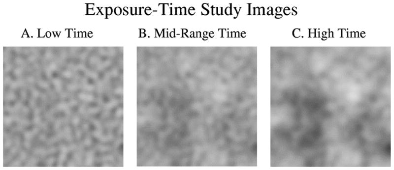
Sample images used in the exposure-time study. The higher-frequency quantum noise component is reduced as exposure time goes up. A. Low-exposure time (experiment 1: W_a/W_q = 0.528). B. Midrange exposure time (experiment 3: W_a/W_q = 29.70). C. High-exposure time (experiment 5: W_a/W_q = 1223.7).

3. Anatomical-Slope Study

The anatomical-slope study consists of five experiments that analyze how the exponent β of the anatomical NPS influences detection performance. The reason for referring to this parameter in terms of a slope has to do with the fact that the anatomical NPS given in Eq. (5) is well approximated by the power law

$${[{\mathbf{N}}_a]}_{kk}\cong W_a{({\rho }_k/{\rho }_a)}^{-\beta }$$ (37)

for ρ_k larger than ρ_a and power-law exponent β > 1. Taking the logarithm of both sides of relation (37) yields a linear equation in ln(ρ_k) with a slope of −β. This sort of slope is often associated with different tissue types as described in Subsection 2.B. The parameter settings for the five experiments in this study are given in Table 3.

Table 3.

Parameter Settings for the Anatomical-Slope Study^a

Exp. No.	As	Wa	Wq	β
1	40.0	519007.	4181.8	4.0
2	40.0	444051.	4181.8	3.5
3	40.0	345010.	4181.8	3.0
4	40.0	226022.	4181.8	2.5
5	40.0	113931.	4181.8	2.0

^aβ refers to the power-law exponent (or anatomical slope) of the anatomical NPS. The cutoff frequency of the Butterworth regularizing filter was held constant at ρ_c = 0.3 across all experiments of the study.

The β parameter controls the rate at which the anatomical NPS falls off to zero. When β is large, the anatomical NPS falls off rapidly, and hence the fluctuations in the images that are due to anatomical variation are highly concentrated in the low-frequency range. Conversely, when β is small, the anatomical NPS falls off much more slowly, indicating the presence of anatomical variability at higher spatial frequencies. The slopes investigated in the study range from −4.0 to −2.0 (hence β = 4.0 to 2.0). Across the studies, W_a has been held constant to fix the contribution of quantum noise to the images. The signal amplitude A_s was fixed as well. The magnitude of the anatomical NPS has been adjusted so that the strength of the noise (measured as the pixel standard deviation) in the images is approximately constant across the experiments. To better capture the effects at slopes near −2.0, where the NPS falls off somewhat more slowly, the cutoff of the Butterworth filter has been set to ρ_c = 0.30 across all five experiments. An example image from experiments 1, 3, and 5 is shown in Fig. 6.

Fig. 6.

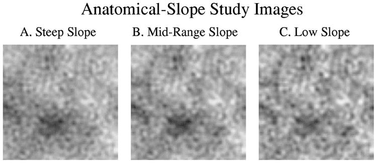
Sample images used in the anatomical-slope study. The anatomical noise extends into higher spatial frequencies as the slope is reduced. A. Steep slope (experiment 1: β = 4.0). B. Midrange slope (experiment 3: β = 3.0). C. Low slope (experiment 5: β = 2.0).

B. Psychophysical Procedure

The monitor on which the psychophysical experiments are conducted is a 17-in. standard DEC Alpha workstation color monitor with a measured screen gamma of 2.8. The images for each experiment were generated by the procedure described in Subsection 2.A with the parameter sets described above. The parameters of the simulations were set so that the images would have a mean (signal-absent) background level of 100 gray levels and a pixel standard deviation less than 30 gray levels. Any pixels that fell outside the gray-level range of the monitor were truncated. Subjects adjusted the room lights and the monitor brightness and contrast to predetermined settings for the experiments. The measured size of a single pixel on the monitor is 0.27 mm; however, the images were magnified by a factor of 4 for display, yielding an effective pixel size of 1.08 mm/pixel. The software for the display of images and the accumulation of observer responses is written entirely in the IDL programming language.

Four observers participated in the psychophysical studies. Two of the observers were paid subjects, naive to the purpose of the research. The other two observers consisted of an author (CKA) and a volunteer from his institution who was also familiar with the research goals. None of the observers had received any formal medical training. Since the tasks investigated here do not require any specific physiological or radiological expertise, we would not expect medical training to have altered the results.

All the observers in these studies received considerable task-specific training before performing the experiments. This training included numerous 2AFC detection experiments in white noise, where the observer performance was compared with that reported in the literature.⁵⁸ Subjects could not proceed to the studies reported here until they consistently achieved performance levels comparable with the published data (40% efficiency with respect to the ideal observer). The fact that observers were able to achieve these predetermined levels of performance indicated reasonable levels of competence among the observers and the adequacy of the monitor for image display in these tasks. In addition, all observers participated in a series of experiments investigating the observer psychometric functions before participating in the experiments reported below (the results of these experiments can be found in related work by Abbey⁴⁸). Finally, before each experiment, a short training session with 50 pairs of trial images was conducted on an independent sample of images generated with the same parameters as those used in the experiment.

Observer performance was assessed in 400 2AFC trials per experimental condition, with each experiment broken into two independent 200-trial sessions to avoid observer fatigue. The observers participated in all the experiments for a given study in the first session before proceeding on to the second session. The different conditions were viewed in random order in each pass through the first and second sittings.

C. Human-Observer Results

The first column of plots in Fig. 7 summarizes human-observer performance in the three studies described above. In these plots, each observer’s detectability [computed from Eq. (21)] is identified by a particular symbol used consistently across the three plots. The dotted curve indicates the average detectability of the four observers. This curve is used (along with error bars) for comparison with the various model observers in the plots to the right of the human-observer data. There is generally good agreement among the observers, with an average coefficient of variation across experiments of 9%.

Fig. 7.

Human-observer performance and model fits. Each row of plots corresponds to the named study (regularization, exposure time, and anatomical slope). Y-axis labels on the left apply across the entire row. The first column of plots shows the performance of all four subjects. For reference, average human-observer performance is plotted with 1-standard-deviation errorbars in all the model-observer plots as well. The second column gives the performance of the Hotelling observer, the nonprewhitening (NPW) observer, the region-of-interest (ROI) observer, and the eye-filtered nonprewhitening (NPW-eye) observer. The remaining columns show the performance of channelized-Hotelling observers with the square channels (SQR), the three-channel difference of Gaussians (S-DOG), and the ten-channel difference of Gaussians (D-DOG), both with and without internal noise (+noise).

The results of the regularization study are given in the uppermost plot of the first column of Fig. 7. The plot shows the detectability as a function of the filter cutoff frequency ρ_c, defined in Subsection 2.B. Moving from right to left, the performance is relatively flat with a small observed peak at ρ_c = 0.17 followed by a rapid degradation. The peak shows a 13% increase from the lowest level of regularization (ρ_c = 0.45). The shape of the human-performance plot can be interpreted by appealing to the signal and noise spectra of Fig. 2 as follows. The relatively flat performance for ρ_c = 0.45 to ρ_c = 0.23 suggests that the regularizing filter is modulating spectral elements at these high frequencies that have little or no effect on performance. For ρ_c in this range, the attenuated spectral components are almost entirely due to the quantum NPS and hence of little use for performing the task. Since these elements are not being used, modulating them with the Butterworth filter has little effect. As the cutoff of the regularizing filter gets nearer the edge of the signal spectrum, it begins to attenuate noisy spectral components that are influencing the human decision process. The attenuated spectral components are still largely just noise, and hence performance improves as the magnitudes of these components are reduced. At the frequency of the observed peak in human performance (ρ_c = 0.17), the signal spectrum has fallen off by an order of magnitude from its maximum at ρ = 0. So the filter still has only a small effect on the signal, with a larger degree of noise reduction. At higher levels of regularization, performance drops quickly, since the filter begins to attenuate important signal components.

The middle plot in the first column of Fig. 7 gives the human-observer performance in the exposure-time study. The left side of the plot (corresponding to low exposure time) exhibits almost no change in performance, with a slight decrease in performance as the exposure time increases to the right side of the plot. The analogy to exposure time would normally lead us to expect increasing performance. However, recall from Subsection 5.A.2 that the signal amplitude has been fixed throughout the study and does not increase as the magnitude of the anatomical NPS goes up. Hence the task measures the ability to detect a lower-amplitude signal as the exposure time increases. Performance remains approximately constant, even though the signal strength relative to the anatomical background decreases by over 85% between the two ends of the plot.

The human-observer results of the anatomical slope study are plotted on the bottom of the first column of Fig. 7. Observer performance uniformly decreases as the slopes range from −4.0 to −2.0. This decrease in performance may be understood as the effect of the anatomical noise moving into higher spatial frequencies. The NPS values for spatial frequencies in the range of 0.04–0.15 pixels⁻¹ increase on average by a factor of 3.0 as the slope goes from −4 to −2. NPS values for lower spatial frequencies in the range 0.0–0.03 decrease on average by a factor of 3.2. If the observer were heavily weighting the lowest frequencies, we would have expected to see performance improve.

The anatomical-slope study also reinforces the problems associated with performance predictions based on the pixel variance or on other measures that do not take into account pixel-to-pixel correlations. The pixel variance decreases by 19% as the slope goes from −4 to −2, while the signal amplitude stays constant. Therefore a contrast-to-noise ratio based on the signal amplitude and the pixel standard deviation would predict an 11% increase in performance. Instead, we observe a decrease of 44% in average human performance throughout this range. This sort of contraindication has been found previously.³⁴

D. Model-Observer Results

The second column of plots in Fig. 7 gives model-observer performance for the Hotelling observer, the region-of-interest (ROI) observer, the nonprewhitening (NPW) observer, and the eye-filtered nonprewhitening (NPW-Eye) observer. Hotelling-observer performance is computed from Eq. (29), which neglects the effects of image truncation from 128 × 128 to 64 × 64 pixels for display. Since the Hotelling observer is equivalent to the ideal observer in these studies, the performance on 128 × 128-pixel images acts as an upper bound for performance on the truncated images. Hence there is the possibility that performance computed from Eq. (29) overestimates performance on the truncated images. However, we shall see shortly that these effects are small, since the Hotelling-observer performance is nearly equaled by one of the channelized-Hotelling observers that has been computed with image truncation effects.

The Hotelling observer generally matches the trends of the human-observer data, particularly in the exposure-time and anatomical-slope studies. The greatest divergence from the human data is found at the low end of the regularization study. The Hotelling observer does not account for the observed peak in human performance at ρ_c = 0.17 nor for the sharp decrease in performance at lower cutoff frequencies.

The performance of the three NPW models are computed from Eq. (19) with the internal-noise component set to zero ( ${\sigma }_{\epsilon }^2=0$). This choice for the internal-noise component has been made on the basis of absolute performance. Adding internal noise to these models causes them to drop below (in many cases further below) the performance levels of the human observers. A deterministic model observer (one with no internal noise) that is outperformed by human observers has sources of inefficiency not present in the human observers. Hence the predictive value of such models is inherently suspect. By this criterion, the ROI and NPW observers can be rejected because they are consistently outperformed by the human observers. Adding internal noise simply makes them worse.

The NPW-eye model generally outperforms the human observers, except at the low end of the regularization study, where the model approximately equals average human performance. Adding internal noise to the NPW-eye model would cause model-observer performance in this area to drop below the level of human performance. At the high end of the regularization study, the model is nearly equivalent to the ideal observer. In the exposure-time study, the model predicts a substantial peak in performance near an exposure time of 30, which is not present in the human observer data.

Results for a total of six channelized-Hotelling observers are presented in the three remaining columns of Fig. 7. There are two implementations of each of the three channel models—square channels (SQR), sparse difference of Gaussians (S-DOG), and dense difference of Gaussians (D-DOG)—described in Subsection 4.D. Each channel model is implemented with and without internal noise. The observer performance is computed from Eq. (33). The internal noise is presumed to be independent in each channel with variance proportional to the variance of the image noise in the channel. The resulting internal-noise channel covariance matrix is given by

$${\mathbf{K}}_{\epsilon }=c_{\epsilon }\text{diag}({\mathbf{T}}^{\text{t}}{\mathbf{K}}_{\widehat{\mathbf{f}}}\mathbf{T}),$$

where c_ε is a constant of proportionality and diag (T^tK_f̂T) indicates a diagonal matrix with diagonal elements given by the diagonal elements of T^tK_f̂T. For the SQR and S-DOG channel models, c_ε is set to 1.0 in all experiments, which gives good agreement in absolute performance with the human-observer data. Because of the greater number and overlap of the channels, the D-DOG channel model required more internal noise to match human-observer performance. For this model, c_ε is set to 2.5.

The channelized-Hotelling observers give a generally high degree of agreement with the human-observer data. The observer-performance plots show good absolute agreement with human observers when the internal noise is added, and even without internal noise, the observers generally follow the trend of the human-observer data. The largest divergence from the human-observer performance comes from the D-DOG model without internal noise in the regularization study. The observer performance in this case is nearly constant across the cutoff frequency. The addition of internal noise causes this observer to assume the characteristics of the human-observer data.

The D-DOG observer without internal noise gives insight to the effect of image truncation in the implementation of the Hotelling observer. The channel profiles of the D-DOG observer are defined by the size of the truncated images (64 × 64 pixels), and hence they represent an achievable level of performance on the truncated images. Therefore the performance of the D-DOG channelized-Hotelling observer acts as a lower bound on performance for the Hotelling observer for the truncated images. As described above, the performance of the Hotelling observer given in the second row of the plots acts as an upper bound for performance on truncated images. Since the two observers give nearly identical results, we can conclude that truncation effects do not greatly effect the performance of the Hotelling observer.

6. SUMMARY AND CONCLUSIONS

The purpose of this work has been to investigate observer performance in detection tasks that are similar in design to previously reported results for noise-limited detection but oriented more toward tomographic image reconstruction. This has been done by considering correlated Gaussian noise that has a ramp-spectrum component to approximate the effects of the reconstruction process on quantum noise in projection data, as well as a low-pass component to roughly simulate patient-to-patient variability in reconstructed images. The effect of regularization that is due to a reconstruction algorithm is implemented as a low-pass Butterworth filter that affects both the signal profile and the correlation structure of the noise. While this is a crude model of the variability present in clinical SPECT or PET reconstructed images, we feel that it is sufficient to achieve our goal of understanding factors that influence human-observer performance and seeing if these effects are captured in the performance of model observers.

A total of 17 detection experiments have been organized into three studies to generate the results of this work. The studies investigate the effects of parameters related to regularization and exposure time and a parameter related to tissue properties that is called the anatomical slope. Performance has been assessed for human observers through psychophysical studies and for a number of model observers through ensemble calculations utilizing principles from signal detection theory. The human-observer results of these studies are relatively consistent between observers (9% coefficient of variation) and highly dependent on the experimental parameters.

A total of ten model observers have been tested for agreement with the human-observer data including the Hotelling observer—the ideal observer for these experiments, three nonprewhitening observers that do not take into account pixel-to-pixel correlations in the images, and six implementations of the channelized-Hotelling observer. The Hotelling and nonprewhitening observers generally do not reproduce important features of the human-observer data. Hence we can conclude that these models are not good predictors of human-observer performance in images with structured noise similar to that used here. The channelized-Hotelling observers give generally good agreement with the human-observer data, with good matching performance on an absolute scale when internal noise is added to the channel responses. Hence the channels appear to be a good mechanism for implementing a suboptimal observer that is able to partially adapt to image statistics.

The fact that the three channelized-Hotelling observers all make similar predictions for these experiments indicate that there is still work to be done in distinguishing between observers as predictors of human-observer performance. A broader set of experiments may serve to identify an optimal and robust set of channels for predicting human performance. An alternative approach is to estimate human-observer templates directly as described recently by Abbey et al.^59,60 Under this approach, estimated human-observer templates could be directly compared with model-observer templates.

References

- 1.Barrett HH, Smith WE, Myers KJ, Milster TD, Fiete RD. Quantifying the performance of imaging systems. In: Dwyer SJ, Schneider RH, editors. Application of Optical Instrumentation in Medicine XIII; Proc. SPIE; 1985. pp. 65–69. [Google Scholar]
- 2.Myers KJ, Barrett HH, Borgstrom MC, Cargill EB, Clough AV, Fiete RD, Milster TD, Patton DD, Paxman RG, Seeley GW, Smith WE, Stempski MO. A systematic approach to the design of diagnostic systems for nuclear medicine. In: Bacharach SL, editor. Information Processing in Medical Imaging: Proceedings of the Ninth Conference. Martinus Nijhoff; Dordrecht, The Netherlands: 1986. pp. 431–444. [Google Scholar]
- 3.Barrett HH. Objective assessment of image quality: effects of quantum noise and object variability. J Opt Soc Am A. 1990;7:1266–1278. doi: 10.1364/josaa.7.001266. [DOI] [PubMed] [Google Scholar]
- 4.Barrett HH, Gordon SK, Hershel RS. Statistical limitations in transaxial tomography. Comput Biol Med. 1976;6:307–323. doi: 10.1016/0010-4825(76)90068-8. [DOI] [PubMed] [Google Scholar]
- 5.Riederer SJ, Pelc NJ, Chessler DA. The noise power spectrum in computed x-ray tomography. Phys Med Biol. 1978;23:446–454. doi: 10.1088/0031-9155/23/3/008. [DOI] [PubMed] [Google Scholar]
- 6.Barrett HH, Swindell W. Radiological Imaging: The Theory of Image Formation, Detection, and Processing. Academic; New York: 1981. [Google Scholar]
- 7.Cargill EB. PhD dissertation. University of Arizona; Tucson, Ariz: 1989. A mathematical liver model and its application to system optimization and texture analysis. [Google Scholar]
- 8.Wei D, Chan HP, Helvie MA, Sahiner B, Petrick N, Adler DD, Goodsitt MM. Multiresolution texture analysis for classification of mass and normal breast tissue on digital mammograms. In: Loew MH, editor. Medical Imaging: Image Processing; Proc. SPIE; 1995. pp. 606–611. [DOI] [PubMed] [Google Scholar]
- 9.Bochud FO, Abbey CK, Eckstein MP. Statistical texture synthesis of mammographic images with clustered lumpy backgrounds. Opt Expr. 1998;4:33–43. doi: 10.1364/oe.4.000033. [DOI] [PubMed] [Google Scholar]
- 10.Burgess AE. Mammographic structure: data preparation and spatial statistics analysis. In: Hanson KM, editor. Medical Imaging: Image Processing; Proc. SPIE; 1999. pp. 642–653. [Google Scholar]
- 11.Bochud FO, Abbey CK, Eckstein MP. Further investigation of the phase spectrum on visual detection in structured backgrounds. In: Krupinski E, editor. Medical Imaging: Image Perception and Performance; Proc. SPIE; 1999. pp. 273–281. [Google Scholar]
- 12.Bochud FO, Abbey CK, Eckstein MP. Visual signal detection in structured backgrounds. III. Calculation of figures of merit for model observers in statistically non-stationary backgrounds. J Opt Soc Am A. 2000;17:193–205. doi: 10.1364/josaa.17.000193. [DOI] [PubMed] [Google Scholar]
- 13.Burgess AE, Li X, Abbey CK. Visual signal detectability with two noise components: anomalous masking effects. J Opt Soc Am A. 1997;14:2420–2442. doi: 10.1364/josaa.14.002420. [DOI] [PubMed] [Google Scholar]
- 14.Bracewell R. The Fourier Transform and Its Applications. McGraw-Hill; New York: 1965. [Google Scholar]
- 15.Kijewski MF, Judy PF. The noise power spectrum of CT images. Phys Med Biol. 1987;32:565–575. doi: 10.1088/0031-9155/32/5/003. [DOI] [PubMed] [Google Scholar]
- 16.Voss RF. Fractals in nature: from characterization to simulation. In: Barnsley MF, Devaney RL, Mandelbrot BB, editors. The Science of Fractal Images. Springer-Verlag; New York: 1988. [Google Scholar]
- 17.Heine JJ, Deans SR, Clarke LP. Multiresolution probability analysis of random fields. J Opt Soc Am A. 1999;16:6–16. [Google Scholar]
- 18.Rolland JP, Barrett HH. Effect of random background inhomogeneity on observer detection performance. J Opt Soc Am A. 1992;9:649–658. doi: 10.1364/josaa.9.000649. [DOI] [PubMed] [Google Scholar]
- 19.Burgess AE. Statistically defined backgrounds: performance of a modified nonprewhitening matched filter model. J Opt Soc Am A. 1994;11:1237–1242. doi: 10.1364/josaa.11.001237. [DOI] [PubMed] [Google Scholar]
- 20.Burgess AE, Li X, Abbey CK. Nodule detection in two component noise: toward patient structure. In: Kundel HL, editor. Medical Imaging: Image Perception; Proc. SPIE; 1997. pp. 2–13. [Google Scholar]
- 21.Samei E, Flynn MJ, Beue GH, Peterson E. Comparison of observer performance for real and simulated nodules in chest radiography. In: Kundel HL, editor. Medical Imaging: Image Perception; Proc. SPIE; 1996. pp. 60–70. [Google Scholar]
- 22.Mardia KV, Kent JT, Bibby JM. Multivariate Analysis. Academic; San Diego, Calif: 1979. pp. 62–66. [Google Scholar]
- 23.Judy PF, Swensson RG. Detection of small focal lesions in CT images: effects of reconstruction filters and visual display windows. Br J Radiol. 1985;58:137–145. doi: 10.1259/0007-1285-58-686-137. [DOI] [PubMed] [Google Scholar]
- 24.Judy PF, Swensson RG. Display thresholding of images and observer detection performance. J Opt Soc Am A. 1987;4:954–965. doi: 10.1364/josaa.4.000954. [DOI] [PubMed] [Google Scholar]
- 25.Judy PF, Swensson RG, Nawfel RD, Chan KH, Seltzer SE. Contrast-detail curves for liver CT. Med Phys. 1992;19:1167–1174. doi: 10.1118/1.596791. [DOI] [PubMed] [Google Scholar]
- 26.Pelli D. PhD dissertation. Cambridge U. Press; Cambridge, UK: 1981. Effects of visual noise. [Google Scholar]
- 27.Burgess AE, Colborne B. Visual signal detection. IV. Observer inconsistency. J Opt Soc Am A. 1988;5:617–627. doi: 10.1364/josaa.5.000617. [DOI] [PubMed] [Google Scholar]
- 28.Eckstein MP, Ahumada AJ, Watson AB. Visual signal detection in structured backgrounds. II. Effects of contrast gain control, background variations, and white noise. J Opt Soc Am A. 1997;13:1777–1787. doi: 10.1364/josaa.14.002406. [DOI] [PubMed] [Google Scholar]
- 29.Barrett HH, Yao J, Rolland JP, Myers KJ. Model observers for the assessment of image quality. Proc Natl Acad Sci. 1993;90:9758–9765. doi: 10.1073/pnas.90.21.9758. [DOI] [PMC free article] [PubMed] [Google Scholar]
- 30.Barrett HH, Gooley TA, Girodias KA, Rolland JP, White TA, Yao J. Linear discriminants and image quality. Image Vis Comput. 1992;10:451–460. [Google Scholar]
- 31.Green DM, Swets JA. Signal Detection Theory and Psychophysics. Wiley; New York: 1966. [Google Scholar]
- 32.Macmillan NA, Creelman CD. Detection Theory: A Users Guide. Cambridge U. Press; New York: 1991. [Google Scholar]
- 33.Barrett HH, Abbey CK, Clarkson E. Objective assessment of image quality. III. ROC metrics, ideal observers, and likelihood generating functions. J Opt Soc Am A. 1998;15:1520–1535. doi: 10.1364/josaa.15.001520. [DOI] [PubMed] [Google Scholar]
- 34.Myers KJ. PhD dissertation. University of Arizona; Tucson, Ariz: 1985. Visual perception in correlated noise. [Google Scholar]
- 35.Myers KJ, Barrett HH. The addition of a channel mechanism to the ideal-observer model. J Opt Soc Am A. 1987;4:2447–2457. doi: 10.1364/josaa.4.002447. [DOI] [PubMed] [Google Scholar]
- 36.Burgess AE. The Rose model revisited. J Opt Soc Am A. 1999;16:633–646. doi: 10.1364/josaa.16.000633. [DOI] [PubMed] [Google Scholar]
- 37.Loo LN, Doi K, Metz CE. A comparison of physical image quality indices and observer performance in the radiographic detection of nylon beads. Phys Med Biol. 1984;29:837–856. doi: 10.1088/0031-9155/29/7/007. [DOI] [PubMed] [Google Scholar]
- 38.Ishida M, Doi K, Loo LN, Metz CE, Lehr JL. Digital image processing: effect on detectability of simulated low-contrast radiographic patterns. Radiology. 1984;150:569–575. doi: 10.1148/radiology.150.2.6691118. [DOI] [PubMed] [Google Scholar]
- 39.Loo LN, Doi K, Metz CE. Investigation of basic imaging properties in digital radiography. 4. Effect of unsharp masking on the detectability of simple patterns. Med Phys. 1985;29:209–214. doi: 10.1118/1.595775. [DOI] [PubMed] [Google Scholar]
- 40.Myers KJ, Barrett HH, Borgstrom MC, Patton DD, Seeley GW. Effect of noise correlation on the detectability of disk signals in medical imaging. J Opt Soc Am A. 1985;2:1752–1759. doi: 10.1364/josaa.2.001752. [DOI] [PubMed] [Google Scholar]
- 41.Judy PF, Swensson RG. Detectability of lesions of various sizes on CT images. In: Dwyer SJ, Schneider RH, editors. Application of Optical Instrumentation in Medicine XIII; Proc. SPIE; 1985. pp. 38–42. [Google Scholar]
- 42.Judy PF, Swensson RG. Size discrimination of features on CT images. In: Dwyer SJ, Schneider RH, editors. Application of Optical Instrumentation in Medicine XIV; Proc. SPIE; 1986. pp. 225–230. [Google Scholar]
- 43.Barten PGJ. The SQRI method: a new method for the evaluation of visible resolution on a display. Proc Soc Inf Disp. 1987;28:253–262. [Google Scholar]
- 44.Fiete RD, Barrett HH, Smith WE, Myers KJ. The Hotelling trace criterion and its correlation with human observer performance. J Opt Soc Am A. 1987;4:945–953. doi: 10.1364/josaa.4.000945. [DOI] [PubMed] [Google Scholar]
- 45.Campbell FW, Robson JG. Application of Fourier analysis to the visibility of gratings. J Physiol (London) 1968;197:551–566. doi: 10.1113/jphysiol.1968.sp008574. [DOI] [PMC free article] [PubMed] [Google Scholar]
- 46.Sachs MB, Nachmias J, Robson JG. Spatial-frequency channels in human vision. J Opt Soc Am. 1971;61:1176–1186. doi: 10.1364/josa.61.001176. [DOI] [PubMed] [Google Scholar]
- 47.Graham N. Complex channels, early nonlinearities, and normalization in texture segregation. In: Landy MS, Movshon JA, editors. Computational Models of Visual Processing. MIT Press; Cambridge, Mass: 1990. pp. 273–290. [Google Scholar]
- 48.Abbey CK. PhD dissertation. University of Arizona; Tucson, Ariz: 1998. Assessment of reconstructed images. [Google Scholar]
- 49.Abbey CK, Bochud FO. Modeling visual detection tasks in correlated noise with linear model observers. In: Beutel J, Kundel HL, Van Metter RL, editors. Handbook of Medical Imaging. Vol. 1. SPIE Press; Bellingham, Wash: 2000. pp. 629–654. [Google Scholar]
- 50.Barrett HH, Abbey CK, Gallas B, Eckstein MP. Stabilized estimates of Hotelling observer performance in patient-structured noise. In: Kundel HL, editor. Medical Imaging: Image Perception; Proc. SPIE; 1998. pp. 27–43. [Google Scholar]
- 51.Abbey CK, Barrett HH. Linear iterative reconstruction algorithms: study of observer performance. In: Bizais Y, Barrilot C, Di Paola R, editors. Proceedings of the 14th International Conference on Information Processing in Medical Imaging. Kluwer Academic; Dordrecht, The Netherlands: 1995. pp. 65–76. [Google Scholar]
- 52.Abbey CK, Barrett HH, Wilson DW. Observer signal-to-noise ratios for the ML-EM algorithm. In: Kundel HL, editor. Medical Imaging: Image Perception; Proc. SPIE; 1996. pp. 47–58. [DOI] [PMC free article] [PubMed] [Google Scholar]
- 53.Wilson HR, Giese SC. Threshold visibility of frequency gradient patterns. Vision Res. 1977;17:1177–1190. doi: 10.1016/0042-6989(77)90152-3. [DOI] [PubMed] [Google Scholar]
- 54.Wilson H, Bergen J. A four mechanism model for threshold spatial vision. Vision Res. 1979;19:19–32. doi: 10.1016/0042-6989(79)90117-2. [DOI] [PubMed] [Google Scholar]
- 55.Watson AB. Detection and recognition of simple spatial forms. In: Sander OJ, Sleigh AJ, editors. Physical and Biological Processing of Images. Springer-Verlag; Berlin: 1983. [Google Scholar]
- 56.Daly S. The visual differences predictor: an algorithm for the assessment of image fidelity. In: Watson AB, editor. Digital Images and Human Vision. MIT Press; Cambridges, Mass: 1993. pp. 179–206. [Google Scholar]
- 57.Eckstein MP, Whiting JS. Lesion detection in structured noise. Acad Radiol. 1995;2:249–253. doi: 10.1016/s1076-6332(05)80174-6. [DOI] [PubMed] [Google Scholar]
- 58.Burgess AE, Ghandeharian H. Visual signal detection. I. Ability to use phase information. J Opt Soc Am A. 1984;1:900–905. doi: 10.1364/josaa.1.000900. [DOI] [PubMed] [Google Scholar]
- 59.Abbey CK, Eckstein MP, Bochud FO. Estimation of human-observer templates for 2 alternative forced choice tasks. In: Krupinski EA, editor. Medical Imaging: Image Perception and Performance; Proc. SPIE; 1999. pp. 284–295. [Google Scholar]
- 60.Abbey CK, Eckstein MP. Estimates of human-observer templates for simple detection tasks in correlated noise. In: Krupinski EA, editor. Medical Imaging: Image Perception and Performance; Proc. SPIE; 2000. pp. 70–77. [Google Scholar]