

Abstract
Although great progress in genome-wide association studies (GWAS) has been made, the significant SNP associations identified by GWAS account for only a few percent of the genetic variance, leading many to question where and how we can find the missing heritability. There is increasing interest in genome-wide interaction analysis as a possible source of finding heritability unexplained by current GWAS. However, the existing statistics for testing interaction have low power for genome-wide interaction analysis. To meet challenges raised by genome-wide interactional analysis, we have developed a novel statistic for testing interaction between two loci (either linked or unlinked). The null distribution and the type I error rates of the new statistic for testing interaction are validated using simulations. Extensive power studies show that the developed statistic has much higher power to detect interaction than classical logistic regression. The results identified 44 and 211 pairs of SNPs showing significant evidence of interactions with FDR<0.001 and 0.001<FDR<0.003, respectively, which were seen in two independent studies of psoriasis. These included five interacting pairs of SNPs in genes LST1/NCR3, CXCR5/BCL9L, and GLS2, some of which were located in the target sites of miR-324-3p, miR-433, and miR-382, as well as 15 pairs of interacting SNPs that had nonsynonymous substitutions. Our results demonstrated that genome-wide interaction analysis is a valuable tool for finding remaining missing heritability unexplained by the current GWAS, and the developed novel statistic is able to search significant interaction between SNPs across the genome. Real data analysis showed that the results of genome-wide interaction analysis can be replicated in two independent studies.
Author Summary
It is expected that genome-wide interaction analysis can be a possible source of finding heritability unexplained by current GWAS. However, the existing statistics for testing interaction have low power for genome-wide interaction analysis. To meet challenges raised by genome-wide interactional analysis, we develop a novel statistic for testing interaction between two loci (either linked or unlinked) and validate the null distribution and the type I error rates of the new statistic through simulations. By extensive power studies we show that the developed novel statistic has much higher power to detect interaction than the classical logistic regression. To provide evidence of gene–gene interactions as a possible source of the missing heritability unexplained by the current GWAS, we performed the genome-wide interaction analysis of psoriasis in two independent studies. The preliminary results identified 44 and 211 pairs of SNPs showing significant evidence of interactions with FDR<0.001 and 0.001<FDR<0.003, respectively, which were common in two independent studies. These included five interacting pairs of SNPs, some of which were located in the target sites: LST1/NCR3, CXCR5/BCL9L and GLS2 of miR-324-3p, miR-433, and miR-382, and 15 pairs of interacting SNPs that had nonsynonymous substitutions.
Introduction
In the past three years, about 400 genome-wide association studies (GWAS) that focused largely on individually testing the associations of single SNP with diseases have been conducted [1]. These studies have identified more than 531 SNPs associated with different traits or diseases [2] and have provided substantial information for understanding disease mechanisms. Despite the progress that has been made, the significant SNP associations identified by GWAS account for only a few percent of the genetic variance which begs the question where and how the missing heritability can be identified [3], [4]. Possible explanations include [1], [4]:
The previous GWAS are mainly based on the common disease, common variant hypothesis. However, in addition to single nucleotide polymorphisms (SNPs) with a minor allele frequency (MAF) greater than 1%, there are other classes of human genetic variation including: (a) rare variants that are defined as mutations with a MAF of less than 1% and (b) structural variants including copy number variants (CNVs) and copy neutral variation such as inversions and translocations. Common diseases can also be caused by multiple rare mutations, each with a low marginal genetic effect. A more realistic model is that the entire spectrum of genetic variants ranging from rare to common contributes to disease susceptibility.
Most of current GWAS have focused on SNP analysis in which each variant is tested for association individually. However, common disease often arises from the combined effect of multiple loci within a gene or interaction of multiple genes within a pathway. If we only consider the most significant SNPs, the genetic variants that jointly have significant impact on risk, but individually make only a small contribution, will be missed.
The power of the widely used statistics for detection of gene-gene interaction and gene-environment interactions is low. Many interacting SNPs have not been identified.
Another way to discover the missing heritability of complex diseases is to investigate gene-gene and gene-environment interaction. Disease development is a dynamic process of gene-gene and gene-environment interactions within a complex biological system which is organized into interacting networks [5]. Modern complexity theory assumes that the complexity is attributed to the interactions among the components of the system, therefore, interaction has been considered as a sensible measure of complexity of the biological systems. The more interactions between the components there are, the more complex the system is. The disease may be caused by joint action of multiple loci. Motivation for studying statistical interaction is to provide increased power for detecting joint acting effects of interacting loci than testing for only marginal association of each of the loci individually. Screening for only main effects might miss the vast majority of the genetic variants that interact with each other and with environment to cause diseases [6]. We argue that the interactions hold a key for dissecting the genetic structure of complex diseases and elucidating the biological and biochemical pathway underlying the diseases [7], [8]. Ignoring gene-gene and gene-environment interactions will likely obscure the detection of genetic effects and may lead to inconsistent association results across studies [9], [10].
GWAS in which several hundred thousands or even a millions of SNPs are typed in thousands of individuals provide unprecedented opportunities for systematic exploration of the universe of variants and interactions in the entire genome and also raise several serious challenges for genome-wide interaction analysis. The first challenge comes from the problems imposed by multiple testing. Even for investigating pair-wise interaction, the total number of tests for interaction between all possible SNPs across the genome will be extremely large. Bonferroni-corrected P-values for ensuring genome-wide significance level of 0.05 will be too small to reach. The second challenge is the need for computationally simple statistics for testing interactions. The simplest way to search for interactions between two loci is to test all possible two-locus interactions. This exhaustive search demands large computations. Therefore, the computational time of each two-locus interaction test should be short. The third challenge is the power of the statistics for testing interaction. To ensure the genome-wide significance, the statistics should have high power to detect interaction. Developing simple and efficient analytic methods for evaluation of the gene-gene interactions is critical to the success of genome-wide gene-gene interaction analysis. Finally, the fourth challenge is replication of the finding of such interactions in independent studies.
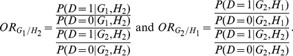
This report will attempt to meet these challenges, at least in part. To achieve this, we first should define a good measure of gene-gene interaction. Despite current enthusiasm for investigation of gene-gene interactions, published results that document these interactions in humans are limited and the essential issue of how to define and detect gene-gene interactions remains unresolved. Over the last three decades, epidemiologists have debated intensely about how to define and measure interaction in epidemiologic studies [7], [8], [11]–[15]; The concept of gene-gene interactions is often used, but rarely specified with precision [16]. In general, statistical gene-gene interaction is defined as departure from additive or multiplicative joint effects of the genetic risk factors [17]. It is increasingly recognized that statistical interactions are scale dependent [18]. In other words, how to define the effects of a risk factor and how to measure departure from the independence of effects will greatly affect assessment of gene-gene interaction. The most popular scale upon which risk factors are measured in case-control studies is odds-ratio. The traditional odds-ratio is defined in terms of genotypes at two loci. Similar to two-locus association analysis where only genotype information at two loci is used, odds-ratio defined by genotypes for testing interaction will not employ allelic association information. However, it is known that interaction between two loci will generate allelic associations in some circumstances [19]. Since they do not use allelic association information between two loci, the statistical methods based on the odds-ratio that is defined in terms of genotypes will have less power to detect interaction. To overcome this limitation, we will define odds-ratio in terms of a pseudohaplotype (which is defined as two alleles located on the same paternal or maternal chromosomes) for measuring interaction, and then we will investigate its properties and develop a statistic based on pseudohaplotype defined odds-ratio for testing interaction between two loci (either linked or unlinked).
To demonstrate that the pseudohaplotype odds-ratio interaction measure-based statistic for detection of interaction between two loci will not cause false positive problems, we then investigate type I error rates. To reveal the merit and limitation of the pseudohaplotype odds-ratio interaction measure-based statistic for detection of interaction, we will compare its power for detecting interaction with the traditional logistic regression and “fast-epistasis” in PLINK [20].
Although nearly 400 GWAS have been documented, few genome-wide interaction analyses have been performed and few findings of significant interaction reported [8], [21], [22]. Emily et al [23] tested about 3,107,904–3,850,339 pairs of SNPs located in genes with potential protein-protein interaction and reported four significant cases of interactions, one in each of Crohn's Disease, bipolar disorder, hypertension and rheumatoid arthritis in the WTCCC dataset, but these have not been replicated. To further evaluate the performance of our new statistic and test the feasibility of genome-wide interaction analysis, the presented statistic was applied to interaction analysis of two independent GWAS datasets of psoriasis where 1,266,378,301 pairs of SNPs from 50,327 SNPs in the first dataset and 1,243,782,750 pairs of SNPs from 49,876 SNPs in the second dataset were tested for interactions. These SNPs in the datasets were selected from 501 pathways assembled from KEGG [24] and Biocarta (http://www.biocarta.com) pathway databases. A program for using the developed statistic to test interaction which was implemented by C++ can be downloaded from our website http://www.sph.uth.tmc.edu/hgc/faculty/xiong/index.htm.
Methods
A case-control study design for detection of interaction between two loci (SNPs) where two loci can be either linked or unlinked were considered. The statistics for testing interaction are usually motivated by the measure of interaction. The widely used logistic regression methods for detection of gene-gene interaction are based on then odds-ratio measure of interaction. Traditional additive and multiplicative odds ratio measures of interaction are defined in terms of genotypes at two loci. In this report, a novel statistic for testing interaction between two loci is based on multiplicative odds-ratio measures defined in terms of pseudohaplotypes. For the convenience of presentation, we first briefly introduce the odds ratio interaction measure in terms of genotypes, alleles, and then present the odds ratio measure in terms of pseudohaplotypes.
Genotype-Based Odds Ratio Multiplicative Interaction Measure
Consider two loci: G and H. Assume that the codes  and
and
 denote whether an individual is a carrier (non-carrier)
of the susceptible genotypes at the loci G and H, respectively. Let D denote
disease status where
denote whether an individual is a carrier (non-carrier)
of the susceptible genotypes at the loci G and H, respectively. Let D denote
disease status where  indicates an
affected (unaffected) individual. Consider the following logistic
model:
indicates an
affected (unaffected) individual. Consider the following logistic
model:
| (1) |
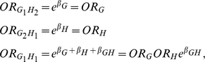
The odds-ratio associated with G for
nonsusceptible genotype at the locus H  is defined
as
is defined
as
Similarly, the odds-ratio associated with H for
nonsusceptible genotype at the locus G  is defined
as
is defined
as
The odds-ratio associated with susceptibility at G and H
compared to the baseline category  and
and
 is then computed as
The odds for baseline
category  and
and  are determined
as
are determined
as
From equation (1), we clearly have
Define a multiplicative interaction measure between two loci G and H as
| (2 – A) |
It is clear that
| (2 – B) |
If  , i.e., there is no
interaction between loci G and H, then
, i.e., there is no
interaction between loci G and H, then  . This shows that
the logistic regression coefficient for interaction term
. This shows that
the logistic regression coefficient for interaction term
 is equivalent to the interaction measure defined as log
odds-ratio. The interaction measure
is equivalent to the interaction measure defined as log
odds-ratio. The interaction measure  can also be
written as
can also be
written as
 |
The values of odds-ratio defined in terms of genotypes depends on how to code
indicator variables G and H. Suppose that alleles
 and
and  are alleles that
increase disease risk. For a recessive model, G is coded as 1 if the genotype is
are alleles that
increase disease risk. For a recessive model, G is coded as 1 if the genotype is
 , otherwise, G is coded as 0. For a dominant model, G is
coded as 1 if the genotypes are either
, otherwise, G is coded as 0. For a dominant model, G is
coded as 1 if the genotypes are either  or
or
 , otherwise G is coded as 0. The indicator variable H can
be similarly coded. However, in real data analysis, the disease models are
unknown. Especially, the types of two-locus disease models are large [25]. We may have a large
number of possible coding, and many of them may have larger numbers of degrees
of freedom than the allelic model.
, otherwise G is coded as 0. The indicator variable H can
be similarly coded. However, in real data analysis, the disease models are
unknown. Especially, the types of two-locus disease models are large [25]. We may have a large
number of possible coding, and many of them may have larger numbers of degrees
of freedom than the allelic model.
Allele-Based Odds Ratio Multiplicative Interaction Measure
Similar to the odds ratio for genotypes, we can define odds-ratio in terms of
alleles. Let  be the probability that an individual becomes affected
given they have genotype
be the probability that an individual becomes affected
given they have genotype  at locus G and
 at locus H, where
  is either
 or
or  (i.e.
(i.e.
 is a member of the set {
 }) and
 is either
  or
or
 (i.e.
(i.e.  is a member of the
set {
is a member of the
set { }). We can similarly define
 . We then can determine the odds-ratio associated with
the allele
. We then can determine the odds-ratio associated with
the allele  at the G locus and allele
 at the H locus compared to the baseline
 as
as
 |
Similarly, we measure
the odds-ratio associated with the alleles  and
and
 , respectively as
 |
Similar to genotype, we can define a multiplicative interaction measure in terms of log odds-ratio for allele as
which is equivalent to
 |
The “fast-epistasis” test statistic in PLINK (http://pngu.mgh.harvard.edu/~purcell/plink/index.shtml) is defined as
where SE(R) and SE(S) denote the standard deviation of R and S, respectively. Absence of interaction is implied if and only if
This is the basis of the “fast-epistasis” test in PLINK.
Haplotype-Based Odds Ratio Multiplicative Interaction Measure
Suppose that the locus G has two alleles  and
and
 and the locus H has two alleles
 and
and  . Let
. Let
 and
and  be the frequencies
of the alleles
be the frequencies
of the alleles  in the cases and
controls, respectively. For the discussion of convenience, we introduce a
terminology of “pseudohaplotype”. When two loci are linked, a
pseudohaplotype is defined as the regular haplotype. When two loci are unlinked,
a pseudohaplotype is defined as a set of alleles that are located in the same
paternal or maternal chromosomes. The frequencies of a pseudohaplotype can be
estimated by the classical methods for estimation of haplotype frequencies such
as Expectation Maximization (EM) Algorithms. For simplicity, hereafter we will
not make distinction between the haplotype and pseudohaplotype. When two loci
are unlinked, a haplotype is understood as a pseudohaplotype. Let
in the cases and
controls, respectively. For the discussion of convenience, we introduce a
terminology of “pseudohaplotype”. When two loci are linked, a
pseudohaplotype is defined as the regular haplotype. When two loci are unlinked,
a pseudohaplotype is defined as a set of alleles that are located in the same
paternal or maternal chromosomes. The frequencies of a pseudohaplotype can be
estimated by the classical methods for estimation of haplotype frequencies such
as Expectation Maximization (EM) Algorithms. For simplicity, hereafter we will
not make distinction between the haplotype and pseudohaplotype. When two loci
are unlinked, a haplotype is understood as a pseudohaplotype. Let
 ,
,  and
and
 ,
,  denote the
frequencies of haplotypes
denote the
frequencies of haplotypes  and
and
 in the cases and controls, respectively. We define a
penetrance of the haplotype
in the cases and controls, respectively. We define a
penetrance of the haplotype  as the probability
that an individual becomes affected given they have phased genotype
as the probability
that an individual becomes affected given they have phased genotype
 . Let
. Let  be the penetrance
of an individual with the genotype
be the penetrance
of an individual with the genotype  ,
,
 and
and  be the penetrance
of the haplotypes
be the penetrance
of the haplotypes  and
and
 , respectively. The penetrance of the haplotype
 can be mathematically defined as
where
 and
and  are the population
frequencies of the haplotypes
are the population
frequencies of the haplotypes 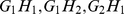 and
and
 , respectively.
 and
and  represent a
genotype coding scheme. Their represented genotypes depend on the specific
genotype coding scheme. It should be noted that the haplotype
represent a
genotype coding scheme. Their represented genotypes depend on the specific
genotype coding scheme. It should be noted that the haplotype
 and
and  and
and
 have different meanings. By the same idea in defining
genotype-based odds ratio in terms of penetrance of combinations of genotypes,
we can determine the odds-ratio associated with the haplotypes
have different meanings. By the same idea in defining
genotype-based odds ratio in terms of penetrance of combinations of genotypes,
we can determine the odds-ratio associated with the haplotypes
 compared to the baseline haplotype
 in terms of penetrance of the haplotypes
as
in terms of penetrance of the haplotypes
as
Similarly, we calculate the odds-ratio associated with the
haplotypes  and
and  , respectively,
as
, respectively,
as
 |
It is noted that replacing  and
and
 in the definition of odds-ratio in terms of genotypes by
 leads to the definition of odds-ratio based on the
haplotypes. However, the values and biological meanings of these two types of
odds-ratios are different.
leads to the definition of odds-ratio based on the
haplotypes. However, the values and biological meanings of these two types of
odds-ratios are different.
Similar to genotypes, we can compute a multiplicative interaction measure in terms of log odds-ratio for haplotypes as
| (3) |
In the absence of interaction, we have
 |
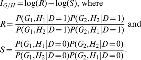
The multiplicative odds-ratio interaction measure in equation (3) is defined by the penetrance of the haplotypes. From case-control data it is difficult to calculate the penetrance of the haplotypes. However, we can show that the multiplicative odds-ratio interaction measure in equation (3) can be reduced to (Text S1, Appendix A)
| (4) |
There are many algorithms and
software to infer the haplotype frequencies in cases and controls. Therefore, we
can easily calculate the multiplicative odds-ratio interaction measure by
equation (4). It can be seen from equation (4) that the absence of interaction
between two loci occurs if and only if the ratio of haplotypes frequencies
 in the cases and the ratio of haplotypes frequencies
 in the controls are equal.
To gain understanding the multiplicative odds-ratio interaction measure, we study several special cases.
Case 1
One of two loci is a marker. If we assume that the locus H is a marker and is not associated with disease, then we have
which implies that
 |
Thus, we obtain  . In other
words, if the locus H is a marker, there is no interaction between two loci
G and H. The interaction measure
. In other
words, if the locus H is a marker, there is no interaction between two loci
G and H. The interaction measure  between two
loci should be equal to zero. Hence, our multiplicative odds-ratio
interaction measure correctly characterizes the marker case.
between two
loci should be equal to zero. Hence, our multiplicative odds-ratio
interaction measure correctly characterizes the marker case.
Case 2
Logistic regression interpretation.
We define two indicator variables:
| (5) |
Then four haplotypes at two loci can be coded as follows:
| G | H | |
| G1H1 | 1 | 1 |
| G1H2 | 1 | 0 |
| G2H1 | 0 | 1 |
| G2H2 | 0 | 0 |
It follows from the logistic regression model in equation (1) that
 |
where odds-ratios  and
and
 are defined in terms of alleles,
i.e.
are defined in terms of alleles,
i.e.
 |
Therefore, the haplotype multiplicative odds-ratio
interaction measure  is equal to
 , which has the same form as that in equation (2-B).
This indicates that if the coding for the genotypes in the genotype
multiplicative odds-ratio interaction measure
, which has the same form as that in equation (2-B).
This indicates that if the coding for the genotypes in the genotype
multiplicative odds-ratio interaction measure
 is replaced by the coding for the haplotypes in
equation (5) then we can obtain the haplotype multiplicative odds-ratio
interaction measure.
is replaced by the coding for the haplotypes in
equation (5) then we can obtain the haplotype multiplicative odds-ratio
interaction measure.
Test Statistics
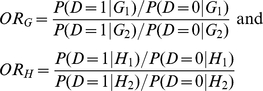
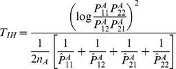
In the previous section we defined the haplotype multiplicative odds-ratio interaction measure, which can be estimated by haplotype frequencies in cases and controls. By the delta method, we can obtain the variance of the estimator of the haplotype odds-ratio interaction measure [26]:
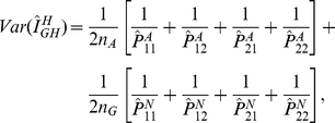 |
where
 and
and  are the number of
sampled individuals in cases and controls. By the standard asymptotic theory we
can define the haplotype odds-ratio interaction measure-based statistic for
testing interaction between two loci:
are the number of
sampled individuals in cases and controls. By the standard asymptotic theory we
can define the haplotype odds-ratio interaction measure-based statistic for
testing interaction between two loci:
 |
(6) |
where  and
and
 are the estimators of the corresponding haplotype
frequencies in cases and controls, respectively. When sample sizes are large
enough to ensure application of large sample theory,
are the estimators of the corresponding haplotype
frequencies in cases and controls, respectively. When sample sizes are large
enough to ensure application of large sample theory,
 is asymptotically distributed as a central
 distribution under the null hypothesis of no interaction
between two loci. Under an alternative hypothesis of of interaction between two
loci being present, the statistic
distribution under the null hypothesis of no interaction
between two loci. Under an alternative hypothesis of of interaction between two
loci being present, the statistic  is asymptotically
distributed as a noncentral
is asymptotically
distributed as a noncentral  distribution with
noncentrality parameter proportional to the haplotype multiplicative odds-ratio
interaction measure. This statistic can be applied to both linked and unlinked
loci. As we explained in Text S1, Appendix B, the proposed statistic
distribution with
noncentrality parameter proportional to the haplotype multiplicative odds-ratio
interaction measure. This statistic can be applied to both linked and unlinked
loci. As we explained in Text S1, Appendix B, the proposed statistic
 is different from the “fast-epistasis” test
in PLINK.
is different from the “fast-epistasis” test
in PLINK.
For the unlinked loci, we can use case only design [27], [28] to study interaction between two loci in which equation is reduced to
 |
(7) |
Results
Null Distribution of Test Statistics
In the previous sections, we have shown that when the sample size is large enough
to apply large sample theory, the distribution of the statistic
 for testing the interaction between two loci under the
null hypothesis of no interaction between them is asymptotically a central
for testing the interaction between two loci under the
null hypothesis of no interaction between them is asymptotically a central
 distribution. To examine the validity of this statement,
we performed a series of simulation studies. MATLAB was used to generate
two-locus genotype data of the sample individuals. A total of 100,000
individuals from a general population with an allele frequency
distribution. To examine the validity of this statement,
we performed a series of simulation studies. MATLAB was used to generate
two-locus genotype data of the sample individuals. A total of 100,000
individuals from a general population with an allele frequency
 ,
,  , haplotype
frequency
, haplotype
frequency  and disequilibrium coefficient
 were generated. A total of 10,000 simulations were
repeated. Type I error rates were calculated by random sampling 500–1,000
individuals as cases and controls from the general population. Table 1 and Table 2 show that the
estimated type I error rates of the statistic
were generated. A total of 10,000 simulations were
repeated. Type I error rates were calculated by random sampling 500–1,000
individuals as cases and controls from the general population. Table 1 and Table 2 show that the
estimated type I error rates of the statistic  for testing
interaction between two loci, assuming
for testing
interaction between two loci, assuming  and
and
 , were not appreciably different from the nominal levels
 ,
,  and
and
 . To further examine the validity of the test statistic,
we constructed Quantile-quantile (Q-Q) plots of the test statistic in datasets 1
and 2 shown in Figures 1A and
1B, where the P-values of the tests were plotted (as −log10
values) as a function of p values from the expected null distribution. Since the
total number of all possible pair-wise tests for interaction between SNPs is too
large to store all the results in computer we only stored P-values
<
. To further examine the validity of the test statistic,
we constructed Quantile-quantile (Q-Q) plots of the test statistic in datasets 1
and 2 shown in Figures 1A and
1B, where the P-values of the tests were plotted (as −log10
values) as a function of p values from the expected null distribution. Since the
total number of all possible pair-wise tests for interaction between SNPs is too
large to store all the results in computer we only stored P-values
< . Consequently, Q-Q plots started with 4. Figures 1A and 1B showed good
agreement with the null distribution.
. Consequently, Q-Q plots started with 4. Figures 1A and 1B showed good
agreement with the null distribution.
Table 1. Type I error rates of the statistic
 to
test for interaction between two loci, assuming
to
test for interaction between two loci, assuming
 .
.
| Sample Size | Nominal levels | ||

|

|

|
|
| 300 | 0.04790 | 0.00995 | 0.00080 |
| 400 | 0.04815 | 0.00820 | 0.00080 |
| 500 | 0.04745 | 0.00930 | 0.00085 |
| 600 | 0.04880 | 0.00850 | 0.00095 |
| 700 | 0.05060 | 0.00920 | 0.00075 |
| 800 | 0.05120 | 0.01015 | 0.00100 |
| 900 | 0.04935 | 0.00805 | 0.00090 |
| 1000 | 0.04860 | 0.00880 | 0.00090 |
Table 2. Type I error rates of the statistic  to test
for interaction between two loci, assuming
to test
for interaction between two loci, assuming
 .
.
| Sample Size | Nominal levels | ||

|

|

|
|
| 300 | 0.04990 | 0.00945 | 0.00120 |
| 400 | 0.04995 | 0.01030 | 0.00085 |
| 500 | 0.05170 | 0.01065 | 0.00080 |
| 600 | 0.05070 | 0.00980 | 0.00100 |
| 700 | 0.04725 | 0.00965 | 0.00113 |
| 800 | 0.04945 | 0.00895 | 0.00075 |
| 900 | 0.04830 | 0.00950 | 0.00080 |
| 1000 | 0.04920 | 0.00975 | 0.00110 |
Figure 1. Quantile-quantile plots for the test statistic
 .
.

(A) Quantile-quantile plots for the test statistic
 in dataset
1. The P-values (<
in dataset
1. The P-values (< ) for the
test are plotted (as −log10 values) as a function of its expected
p values. (B) Quantile-quantile plots for the test statistic
) for the
test are plotted (as −log10 values) as a function of its expected
p values. (B) Quantile-quantile plots for the test statistic
 in dataset
2. The P-values (<
in dataset
2. The P-values (< ) for the
test are plotted (as −log10 values) as a function of its expected
p values.
) for the
test are plotted (as −log10 values) as a function of its expected
p values.
Power Evaluation
To evaluate the performance of the statistic  for detection of
interaction between two loci, we compared the power of the statistic
for detection of
interaction between two loci, we compared the power of the statistic
 to that of the logistic model and the “fast
epistasis” test in PLINK. Power was calculated by simulation. A total of
1,000,000 individuals from a general population with allele frequencies
to that of the logistic model and the “fast
epistasis” test in PLINK. Power was calculated by simulation. A total of
1,000,000 individuals from a general population with allele frequencies
 ,
,  and
and
 and disequilibrium coefficient
 were generated. Two-locus disease models were used to
generate cases and controls, and summarized in Table 3 where odds-ratio was defined in terms
of genotypes. We considered three types of genotype coding. For a recessive
model, homozygous wild type, heterozygous, and homozygous risk increasing
genotypes were coded as 0, 0, 1, respectively. For a dominant model, homozygous
wild type, heterozygous, and homozygous risk increasing genotypes were coded as
0, 1, and 1, respectively. For an additive model, they were coded as 0, 1, and
2, respectively. The genotype coding for the logistic regression matched the
simulation model. The statistic
were generated. Two-locus disease models were used to
generate cases and controls, and summarized in Table 3 where odds-ratio was defined in terms
of genotypes. We considered three types of genotype coding. For a recessive
model, homozygous wild type, heterozygous, and homozygous risk increasing
genotypes were coded as 0, 0, 1, respectively. For a dominant model, homozygous
wild type, heterozygous, and homozygous risk increasing genotypes were coded as
0, 1, and 1, respectively. For an additive model, they were coded as 0, 1, and
2, respectively. The genotype coding for the logistic regression matched the
simulation model. The statistic  in equation (6)
for the case-control version was used to evaluate the power. In the power
simulations, we also assumed that
in equation (6)
for the case-control version was used to evaluate the power. In the power
simulations, we also assumed that  and
and
 . An individual who is randomly sampled from the general
population was assigned to case or control status depending on the two-locus
disease models in Table 3.
The process was repeated until a sample of 1,000 cases and 1,000 controls for
the dominant and additive models, or a sample of 2,000 cases and 2,000 controls
for the recessive model was obtained. A total of 10,000 simulations were
repeated. In Figures
2A–2C, power comparisons among the logistic regression model,
the “fast-epistasis” in PLINK and the statistic
. An individual who is randomly sampled from the general
population was assigned to case or control status depending on the two-locus
disease models in Table 3.
The process was repeated until a sample of 1,000 cases and 1,000 controls for
the dominant and additive models, or a sample of 2,000 cases and 2,000 controls
for the recessive model was obtained. A total of 10,000 simulations were
repeated. In Figures
2A–2C, power comparisons among the logistic regression model,
the “fast-epistasis” in PLINK and the statistic
 under two-locus recessive
 recessive disease
model for significance levels
recessive disease
model for significance levels  ,
,
 and
and  , respectively are
presented. In Figures
3A–3C, power comparisons among the logistic regression model,
the “fast-epistasis” in PLINK and the statistic
, respectively are
presented. In Figures
3A–3C, power comparisons among the logistic regression model,
the “fast-epistasis” in PLINK and the statistic
 under two-locus dominant
 dominant disease
model for significance levels
dominant disease
model for significance levels  ,
,
 and
and  , respectively are
shown. In Figures
4A–4C, power comparisons between the logistic regression model
and the statistic
, respectively are
shown. In Figures
4A–4C, power comparisons between the logistic regression model
and the statistic  under two-locus
additive
under two-locus
additive additive disease
model for significance levels
additive disease
model for significance levels  ,
,
 and
and  , respectively are
demonstrated. Several remarkable features emerge from these Figures. First,
these power Figures indeed demonstrate that the power increases as the measure
of the interaction between two loci increases. The power curves were plotted as
a function of the traditional genotype odds ratio
, respectively are
demonstrated. Several remarkable features emerge from these Figures. First,
these power Figures indeed demonstrate that the power increases as the measure
of the interaction between two loci increases. The power curves were plotted as
a function of the traditional genotype odds ratio
 . We observed that the power curves were a monotonic
increasing function of the genotype odds ratio
. We observed that the power curves were a monotonic
increasing function of the genotype odds ratio  . Therefore, the
test statistic
. Therefore, the
test statistic  can detect the
strength of the interaction between two loci. Second, the test statistic
can detect the
strength of the interaction between two loci. Second, the test statistic
 had much higher power to detect interaction between two
loci than the logistic regression and the “fast-epistasis” test in
PLINK. Third, the more complex the disease models were, the larger the
differences in power between the test statistic
had much higher power to detect interaction between two
loci than the logistic regression and the “fast-epistasis” test in
PLINK. Third, the more complex the disease models were, the larger the
differences in power between the test statistic  , the
“fast-epistasis” test in PLINK and logistic regression that were
observed.
, the
“fast-epistasis” test in PLINK and logistic regression that were
observed.
Table 3. Two-locus disease models.
Recessive Recessive Recessive | |||
| Locus 1\2 | D2D2 | D2d2 | d2d2 |
| D1D1 |
|

|

|
| D1d1 |

|

|

|
| d1d1 |

|

|

|
 ,
,  is the
prevalence of the disease in the population.
is the
prevalence of the disease in the population.
The elements in the Table are the penetrance as a function of the joint genotype at loci 1 and 2 with rows indexing genotype at locus 1 and columns indexing genotype at locus 2.
Figure 2. Power of the statistics for testing interaction between two linked loci under recessive disease model.

(A) The power of the test statistic  , the
“fast-epistasis” in PLINK and logistic regression analysis
for testing interaction between two linked loci as a function of
traditional odds-ratio
, the
“fast-epistasis” in PLINK and logistic regression analysis
for testing interaction between two linked loci as a function of
traditional odds-ratio  under a
two-locus recessive
under a
two-locus recessive recessive
disease model, where the number of individuals in both the case and
control groups is 2,000, the significance level is 0.05, and the
odds-ratios at two loci were
recessive
disease model, where the number of individuals in both the case and
control groups is 2,000, the significance level is 0.05, and the
odds-ratios at two loci were  . (B) The
power of the test statistic
. (B) The
power of the test statistic  , the
“fast-epistasis” in PLINK and logistic regression analysis
for testing interaction between two linked loci as a function of
traditional odds-ratio
, the
“fast-epistasis” in PLINK and logistic regression analysis
for testing interaction between two linked loci as a function of
traditional odds-ratio  under a
two-locus recessive
under a
two-locus recessive recessive
disease model, where the number of individuals in both the case and
control groups is 2,000, the significance level is 0.01, and the
odds-ratios at two loci were
recessive
disease model, where the number of individuals in both the case and
control groups is 2,000, the significance level is 0.01, and the
odds-ratios at two loci were  . (C) The
power of the test statistic
. (C) The
power of the test statistic  , the
“fast-epistasis” in PLINK and logistic regression analysis
for testing interaction between two linked loci as a function of
traditional odds-ratio
, the
“fast-epistasis” in PLINK and logistic regression analysis
for testing interaction between two linked loci as a function of
traditional odds-ratio  under a
two-locus recessive
under a
two-locus recessive recessive
disease model, where the number of individuals in both the case and
control groups is 2,000, the significance level is 0.001, and the
odds-ratios at two loci were
recessive
disease model, where the number of individuals in both the case and
control groups is 2,000, the significance level is 0.001, and the
odds-ratios at two loci were  .
.
Figure 3. Power of the statistics for testing interaction between two linked loci under dominant disease model.

(A) The power of the test statistic  , the
“fast-epistasis” in PLINK and logistic regression analysis
for testing interaction between two linked loci as a function of
traditional odds-ratio
, the
“fast-epistasis” in PLINK and logistic regression analysis
for testing interaction between two linked loci as a function of
traditional odds-ratio  under a
two-locus dominant
under a
two-locus dominant dominant
disease model, where the number of individuals in both the case and
control groups is 1,000, the significance level is 0.05, and the
odds-ratios at two loci were
dominant
disease model, where the number of individuals in both the case and
control groups is 1,000, the significance level is 0.05, and the
odds-ratios at two loci were  . (B) The
power of the test statistic
. (B) The
power of the test statistic  , the
“fast-epistasis” in PLINK and logistic regression analysis
for testing interaction between two linked loci as a function of
traditional odds-ratio
, the
“fast-epistasis” in PLINK and logistic regression analysis
for testing interaction between two linked loci as a function of
traditional odds-ratio  under a
two-locus dominant
under a
two-locus dominant dominant
disease model, where the number of individuals in both the case and
control groups is 1,000, the significance level is 0.01, and the
odds-ratios at two loci were
dominant
disease model, where the number of individuals in both the case and
control groups is 1,000, the significance level is 0.01, and the
odds-ratios at two loci were  . (C) The
power of the test statistic
. (C) The
power of the test statistic  , the
“fast-epistasis” in PLINK and logistic regression analysis
for testing interaction between two linked loci as a function of
traditional odds-ratio
, the
“fast-epistasis” in PLINK and logistic regression analysis
for testing interaction between two linked loci as a function of
traditional odds-ratio  under a
two-locus dominant
under a
two-locus dominant dominant
disease model, where the number of individuals in both the case and
control groups is 1,000, the significance level is 0.001, and the
odds-ratios at two loci were
dominant
disease model, where the number of individuals in both the case and
control groups is 1,000, the significance level is 0.001, and the
odds-ratios at two loci were  .
.
Figure 4. Power of the statistics for testing interaction between two linked loci under additive disease model.

(A) The power of the test statistic  , the
“fast-epistasis” in PLINK and logistic regression for
testing interaction between two linked loci analysis as a function of
traditional odds-ratio
, the
“fast-epistasis” in PLINK and logistic regression for
testing interaction between two linked loci analysis as a function of
traditional odds-ratio  under a
two-locus additive
under a
two-locus additive additive
disease model, where the number of individuals in both the case and
control groups is 1,000, the significance level is 0.05, and the
odds-ratios at two loci were
additive
disease model, where the number of individuals in both the case and
control groups is 1,000, the significance level is 0.05, and the
odds-ratios at two loci were  . (B) The
power of the test statistic
. (B) The
power of the test statistic  , the
“fast-epistasis” in PLINK and logistic regression for
testing interaction between two linked loci analysis as a function of
traditional odds-ratio
, the
“fast-epistasis” in PLINK and logistic regression for
testing interaction between two linked loci analysis as a function of
traditional odds-ratio  under a
two-locus additive
under a
two-locus additive additive
disease model, where the number of individuals in both the case and
control groups is 1,000, the significance level is 0.01, and the
odds-ratios at two loci were
additive
disease model, where the number of individuals in both the case and
control groups is 1,000, the significance level is 0.01, and the
odds-ratios at two loci were  . (C) The
power of the test statistic
. (C) The
power of the test statistic  , the
“fast-epistasis” in PLINK and logistic regression for
testing interaction between two linked loci analysis as a function of
traditional odds-ratio
, the
“fast-epistasis” in PLINK and logistic regression for
testing interaction between two linked loci analysis as a function of
traditional odds-ratio  under a
two-locus additive
under a
two-locus additive additive
disease model, where the number of individuals in both the case and
control groups is 1,000, the significance level is 0.001, and the
odds-ratios at two loci were
additive
disease model, where the number of individuals in both the case and
control groups is 1,000, the significance level is 0.001, and the
odds-ratios at two loci were  .
.
When two loci are unlinked where we do not observe the allelic association
between two loci in the population as a whole, our results also hold. We assumed
the following allele and haplotype frequencies in the population:
 ,
,  and
and
 . Other parameters were defined as before. A total of
10,000 simulations were repeated to simulate the power of three statistics under
three disease models with the significance level
. Other parameters were defined as before. A total of
10,000 simulations were repeated to simulate the power of three statistics under
three disease models with the significance level  . Figures 5A, 5B and 5C showed
the power of three statistics for testing interaction between two unlinked loci
under two-locus recessive
. Figures 5A, 5B and 5C showed
the power of three statistics for testing interaction between two unlinked loci
under two-locus recessive recessive,
dominant
recessive,
dominant dominant, and
additive
dominant, and
additive additive disease
models, respectively. These Figures again demonstrated that the power of the
test statistic
additive disease
models, respectively. These Figures again demonstrated that the power of the
test statistic  was still much
higher than that of the logistic regression and the “fast-epistasis”
test in PLINK. The conclusions still hold for the significance levels
was still much
higher than that of the logistic regression and the “fast-epistasis”
test in PLINK. The conclusions still hold for the significance levels
 and
and  (Data were not
shown).
(Data were not
shown).
Figure 5. Power of the statistics for testing interaction between two unlinked loci.

(A) The power of the test statistic  , the
“fast-epistasis” in PLINK and logistic regression analysis
for testing interaction between two unlinked loci as a function of
traditional odds-ratio
, the
“fast-epistasis” in PLINK and logistic regression analysis
for testing interaction between two unlinked loci as a function of
traditional odds-ratio  under a
two-locus recessive
under a
two-locus recessive recessive
disease model, where the number of individuals in both the case and
control groups is 2,000, the significance level is 0.001, and the
odds-ratios at two loci were
recessive
disease model, where the number of individuals in both the case and
control groups is 2,000, the significance level is 0.001, and the
odds-ratios at two loci were  . (B) The
power of the test statistic
. (B) The
power of the test statistic  , the
“fast-epistasis” in PLINK and logistic regression analysis
for testing interaction between two unlinked loci as a function of
traditional odds-ratio
, the
“fast-epistasis” in PLINK and logistic regression analysis
for testing interaction between two unlinked loci as a function of
traditional odds-ratio  under a
two-locus dominant
under a
two-locus dominant dominant
disease model, where the number of individuals in both the case and
control groups is 1,000, the significance level is 0.001, and the
odds-ratios at two loci were
dominant
disease model, where the number of individuals in both the case and
control groups is 1,000, the significance level is 0.001, and the
odds-ratios at two loci were  . (C) The
power of the test statistic
. (C) The
power of the test statistic  , the
“fast-epistasis” in PLINK and logistic regression analysis
for testing interaction between two unlinked loci as a function of
traditional odds-ratio
, the
“fast-epistasis” in PLINK and logistic regression analysis
for testing interaction between two unlinked loci as a function of
traditional odds-ratio  under a
two-locus additive
under a
two-locus additive additive
disease model, where the number of individuals in both the case and
control groups is 1,000, the significance level is 0.001, and the
odds-ratios at two loci were
additive
disease model, where the number of individuals in both the case and
control groups is 1,000, the significance level is 0.001, and the
odds-ratios at two loci were  .
.
Application to Pathway-Based Genome-Wide Interaction Analysis of Psoriasis
To evaluate its performance for detection of interaction between two loci, the
proposed test statistic  was applied to
interaction analysis of two independent GWAS datasets of psoriasis which were
downloaded from dbGaP. Psoriasis is a common chronic inflammatory skin disease
affecting 2%–3% of the world population. Originally, the first study
included 955 individuals with psoriasis and 693 controls, which is considered as
dataset 1. The second replication study included 466 individuals with psoriasis
and 732 controls, which is designated dataset 2. All cases and controls are of
European origin [29]–[31]. After using PLINK [20] to check for contamination, cryptic
family relationship and non-Caucasian ancestry, 123 samples were excluded.
Subsequently we retained for analysis 915 cases and 675 controls from the first
study and 431 cases and 702 controls from the second study. All 2,723 samples
had been genotyped with the Perlegen 500K array. In the initial dataset, 451,724
SNPs passed quality control (call rate>95%). To further ensure the quality of
the typed SNPs, we used PLINK software to remove the SNPs with >5% missing
genotypes, Hardy-Weinberg disequilibrium (P-values <0.0001), MAF<0.01 and
duplicated markers. In this application, we only considered common SNPs with
MAF>0.01. After quality control filtering, a total of 451,724 SNPs were pruned
to 443,018 and 439,201 SNPs with the average genotyping rate 99.3% in the first
and second studies, respectively.
was applied to
interaction analysis of two independent GWAS datasets of psoriasis which were
downloaded from dbGaP. Psoriasis is a common chronic inflammatory skin disease
affecting 2%–3% of the world population. Originally, the first study
included 955 individuals with psoriasis and 693 controls, which is considered as
dataset 1. The second replication study included 466 individuals with psoriasis
and 732 controls, which is designated dataset 2. All cases and controls are of
European origin [29]–[31]. After using PLINK [20] to check for contamination, cryptic
family relationship and non-Caucasian ancestry, 123 samples were excluded.
Subsequently we retained for analysis 915 cases and 675 controls from the first
study and 431 cases and 702 controls from the second study. All 2,723 samples
had been genotyped with the Perlegen 500K array. In the initial dataset, 451,724
SNPs passed quality control (call rate>95%). To further ensure the quality of
the typed SNPs, we used PLINK software to remove the SNPs with >5% missing
genotypes, Hardy-Weinberg disequilibrium (P-values <0.0001), MAF<0.01 and
duplicated markers. In this application, we only considered common SNPs with
MAF>0.01. After quality control filtering, a total of 451,724 SNPs were pruned
to 443,018 and 439,201 SNPs with the average genotyping rate 99.3% in the first
and second studies, respectively.
Since testing for all possible two-locus interactions across the genome in
genome-wide interaction analysis requires extremely large computation, we
conducted pathway-based genome-wide interaction analysis. We assembled 501
pathways from KEGG [24]
and Biocarta (http://www.biocarta.com). The assignment of SNPs to a gene was
obtained from NCBI human9606 database (version b129). We used the statistic
 to test interactions of all possible pairs of SNPs
located in genes within the assembled 501 pathways. The total number of SNPs in
dataset 1 and dataset 2 being tested was 50,327 and 49,876, respectively. The
serious problem in genome-wide interaction analysis is multiple testing. We used
two strategies to tackle this problem. One is to use false discovery rate (FDR)
[32] to declare
significance of interaction. Another is replication of the findings in two
independent studies, which enhances confidence in interaction tests [22]. We looked for
consistent results across the two independent studies.
to test interactions of all possible pairs of SNPs
located in genes within the assembled 501 pathways. The total number of SNPs in
dataset 1 and dataset 2 being tested was 50,327 and 49,876, respectively. The
serious problem in genome-wide interaction analysis is multiple testing. We used
two strategies to tackle this problem. One is to use false discovery rate (FDR)
[32] to declare
significance of interaction. Another is replication of the findings in two
independent studies, which enhances confidence in interaction tests [22]. We looked for
consistent results across the two independent studies.
In total, 44 pairs of SNPs showed significant evidence of interactions with
FDR<0.001, which roughly corresponds to the P-value
< , in two independent studies (Table S1).
These 44 pairs of SNPs were derived from 71 distinct SNPs located in 60 genes,
including HLA-C, HLA-DRA, HLA-DPA1, LST1, MICB and NOTCH4. Of 44 pairs of SNPs,
only one pair of interacting SNPs: rs2395471 and rs2853950 showed significant
marginal association in two independent studies. An additional 211 pairs of SNPs
with FDR less than 0.003 in the two studies is listed in Table S2.
These interacting SNPs were mainly located in 19 pathways, including a number of
signaling pathways, and immune-related antigen processing and presentation as
well as natural killer cell mediated cytotoxicity pathways (Figure 6). Several remarkable features emerge
from these results. First, although we can observe a few interactions between
SNPs within a gene, the majority of interactions occurred between genes that are
often in different pathways. Since the number of SNPs typed within each gene was
limited, it is unknown whether this is a general rule or just a special case.
Second, a SNP in one gene might interact with multiple SNPs in multiple genes.
For example, SNP rs3131636 in the gene MICB interacting with the SNPs rs915895,
rs443198, rs3134929 in the gene NOTCH4, the SNP rs1052248 in the gene
LAST1/Natural cytotoxicity triggering receptor 3 (NCR3) and the SNP rs1799964 in
the gene LTA/TNF. SNP rs1799964 in the gene LTA/TNF interacting with SNPs
rs3131636, rs3132468 in the gene MICB, SNPs rs9268658 and rs3135392 in the gene
HLA-DRA, SNP rs2227956 in the gene HSPA1L. However, this does not imply that
multiple causal SNPs within a gene will interact with multiple causal SNPs
within another gene. It is quite likely that this is due to LD between the SNPs
within a gene. Third, although interacting SNPs did not form large connected
networks, the interacting SNPs connected pathways into a large complicated
network. This may imply that many genes and pathways are involved in the
development of psoriasis. Fourth, upstream of many pathways included genes with
interacting SNPs. For example, genes MICB, CHRM3, HLA-DRA and CIITA, EPHB1 and
EPHB2, LAMA1 and LANA5, ITGA1, LTBP1, TNF, and FGF20 that contain interacting
SNPs are in the upstream of natural killer cell mediated cytotoxicity, calcium
signaling pathway, antigen processing and presentation, axon guidance,
ECM-receptor interaction pathway, focal adhesion, TGFB pathway, MAPK pathway and
regulation of acting cytoskeleton, respectively. Fifth, most interacting SNPs
are in introns and accounted for 77% of total interacting SNPs.
, in two independent studies (Table S1).
These 44 pairs of SNPs were derived from 71 distinct SNPs located in 60 genes,
including HLA-C, HLA-DRA, HLA-DPA1, LST1, MICB and NOTCH4. Of 44 pairs of SNPs,
only one pair of interacting SNPs: rs2395471 and rs2853950 showed significant
marginal association in two independent studies. An additional 211 pairs of SNPs
with FDR less than 0.003 in the two studies is listed in Table S2.
These interacting SNPs were mainly located in 19 pathways, including a number of
signaling pathways, and immune-related antigen processing and presentation as
well as natural killer cell mediated cytotoxicity pathways (Figure 6). Several remarkable features emerge
from these results. First, although we can observe a few interactions between
SNPs within a gene, the majority of interactions occurred between genes that are
often in different pathways. Since the number of SNPs typed within each gene was
limited, it is unknown whether this is a general rule or just a special case.
Second, a SNP in one gene might interact with multiple SNPs in multiple genes.
For example, SNP rs3131636 in the gene MICB interacting with the SNPs rs915895,
rs443198, rs3134929 in the gene NOTCH4, the SNP rs1052248 in the gene
LAST1/Natural cytotoxicity triggering receptor 3 (NCR3) and the SNP rs1799964 in
the gene LTA/TNF. SNP rs1799964 in the gene LTA/TNF interacting with SNPs
rs3131636, rs3132468 in the gene MICB, SNPs rs9268658 and rs3135392 in the gene
HLA-DRA, SNP rs2227956 in the gene HSPA1L. However, this does not imply that
multiple causal SNPs within a gene will interact with multiple causal SNPs
within another gene. It is quite likely that this is due to LD between the SNPs
within a gene. Third, although interacting SNPs did not form large connected
networks, the interacting SNPs connected pathways into a large complicated
network. This may imply that many genes and pathways are involved in the
development of psoriasis. Fourth, upstream of many pathways included genes with
interacting SNPs. For example, genes MICB, CHRM3, HLA-DRA and CIITA, EPHB1 and
EPHB2, LAMA1 and LANA5, ITGA1, LTBP1, TNF, and FGF20 that contain interacting
SNPs are in the upstream of natural killer cell mediated cytotoxicity, calcium
signaling pathway, antigen processing and presentation, axon guidance,
ECM-receptor interaction pathway, focal adhesion, TGFB pathway, MAPK pathway and
regulation of acting cytoskeleton, respectively. Fifth, most interacting SNPs
are in introns and accounted for 77% of total interacting SNPs.
Figure 6. Interacting SNPs that were located in 19 pathways formed a network.

Each pathway was represented by an ellipse with the number. The SNPs were represented by nodes and placed insight their located pathways. Nearby each SNP there was its RS number and the name of its located gene. The pathway and its harbored SNPs were labeled by the same color. The interacting SNPs were connected by the solid light green lines.
Table 4 listed 15 pairs of interacting SNPs that have non-synonymous substitutions. It is unknown how these nonsynonymous mutations are involved in the pathogenesis of psoriasis. From the literature we know that Plexin C1 receptor is a tumor suppressor gene for melanoma [33], NOTCH4 is involved in schizophrenia [34], Phosphodiesterase 4D (PDE4D) is associated with ischemic stroke [35], HLA-DRA is one of the HLA class II alpha chain genes that plays a central role in antigen processing, and neuregulin 1 (NRG1) has been implicated in diseases such as cancer, schizophrenia and bipolar disorder [36].
Table 4. Interacting SNPs with non-synonymous mutation.
| SNP1(rs) | Gene1 | SNP2(rs) | Gene2 | Dataset 1 | Dataset 2 | Nonsynonymous mutation | Protein Residue | ||
| P-Value | FDR | P-Value | FDR | ||||||
| 10837771 | OR51B4 | 16973321 | RYR3 | 1.20E-07 | 9.00E-04 | 2.28E-07 | 1.34E-03 | rs10837771 | T |
| 7671095 | GRID2 | 10839659 | OR2D3 | 2.00E-08 | 3.97E-04 | 2.82E-08 | 5.29E-04 | rs10839659 | S |
| 1545133 | POLR1B | 8064077 | MYH11 | 6.71E-07 | 1.97E-03 | 5.88E-07 | 2.06E-03 | rs1545133 | L |
| 1958715 | OR4L1 | 3844750 | EFNA5 | 2.15E-08 | 4.10E-04 | 1.25E-07 | 1.03E-03 | rs1958715 | N |
| 1958716 | OR4L1 | 3844750 | EFNA5 | 4.48E-08 | 5.73E-04 | 1.22E-07 | 1.02E-03 | rs1958716 | V |
| 2227956 | HSPA1L | 3135392 | HLA-DRA | 3.20E-10 | 6.02E-05 | 7.82E-10 | 1.05E-04 | rs2227956 | M |
| 2227956 | HSPA1L | 3134929 | NOTCH4 | 7.76E-09 | 2.57E-04 | 2.36E-11 | 2.07E-05 | rs2227956 | M |
| 1799964 | LTA/TNF | 2227956 | HSPA1L | 7.52E-09 | 2.53E-04 | 2.98E-08 | 5.42E-04 | rs2227956 | M |
| 1052248 | LST1/NCR3 | 2227956 | HSPA1L | 8.24E-07 | 2.17E-03 | 1.87E-08 | 4.40E-04 | rs2227956 | M |
| 35258 | PDE4D | 2230793 | IKBKAP | 7.50E-08 | 7.24E-04 | 7.85E-07 | 2.34E-03 | rs2230793 | L |
| 2254524 | LSS | 10860869 | IGF1 | 8.58E-08 | 7.70E-04 | 6.35E-09 | 2.71E-04 | rs2254524 | V |
| 327325 | NRG1 | 3742290 | UTP14C | 7.47E-07 | 2.07E-03 | 5.90E-07 | 2.06E-03 | rs3742290 | A |
| 4253211 | ERCC6 | 10435892 | GABBR2 | 5.60E-07 | 1.81E-03 | 1.11E-09 | 1.23E-04 | rs4253211 | P |
| 940389 | STON1 | 10745676 | PLXNC1 | 2.20E-08 | 4.14E-04 | 7.02E-07 | 2.23E-03 | rs940389 | T |
| 676925 | CXCR5 | 999890 | PIP5K3 | 3.07E-07 | 1.38E-03 | 2.93E-07 | 1.51E-03 | rs999890 | A |
Table 5 includes five interacting pairs of SNPs, one of which falls in the microRNA (MiRNA) binding region. miRNAs, which are 22 nucleotide small RNAs and regulate gene expressions by pairing the miRNA seed region with the target sites, have been implicated in many biological processes including the immune response, biogenesis and tumorigenesis [37]. Mutations in the target sites will affect miRNA activity. A number of studies have identified polymorphisms in the miRNA target sites associated with the diseases [37]. Interestingly, we identified four SNPs in the miRNA (miR-324-3p, miR-433, and miR-382) target sites which interact with five SNPs to contribute to psoriasis. In previous studies, miR-382 has been associated with dermatomyositis, Duchenne muscular dystrophy and Miyoshi myopathy [38], miR-433 and miR-324 with lupus nephritis [39] and miR-433 with Parkinson's disease [40].
Table 5. Five pairs of interacting SNPs, one of which falls in the microRNA binding region.
| SNP1(rs) | Gene 1 | SNP2(rs) | Gene 2 | Dataset 1 | Dataset 2 | MicroRNA Binding Site | ||
| P-Value | FDR | P-Value | FDR | |||||
| 1052248 | LST1/NCR3 | 2227956 | HSPA1L | 8.24E-07 | 2.17E-03 | 1.87E-08 | 4.40E-04 | rs1052248 (miR-324-3p) |
| 1052248 | LST1/NCR3 | 3131636 | MICB | 5.56E-13 | 3.03E-06 | 7.76E-10 | 1.04E-04 | rs1052248 (miR-324-3p) |
| 676925 | CXCR5/BCL9L | 999890 | PIP5K3 | 3.07E-07 | 1.38E-03 | 2.93E-07 | 1.51E-03 | rs676925 (miR-382) |
| 163274 | ACSM1 | 2638315 | GLS2 | 8.16E-07 | 2.16E-03 | 9.14E-07 | 2.51E-03 | rs2638315 (miR-433) |
| 2072619 | MYH11 | 3822711 | GALNT10 | 1.83E-07 | 1.09E-03 | 3.77E-08 | 6.03E-04 | rs3822711 (miR-324-3p) |
Some researchers suggest that in genome-wide interaction analysis only SNPs with large or mild marginal genetic effects should be tested for interaction. To examine whether this strategy will miss detection of interacting SNPs, we showed in Table 6 the 20 top pairs of interacting SNPs and in Table S3 all pairs of interacting SNPs with FDR less than 0.003. Surprisingly, 75% of SNPs with P-values (in dataset 1) larger than 0.2 and 44% of SNPs with P-values larger than 0.5 in two studies were observed in Table S3. Table 6 and Table S3 strongly demonstrated that while both SNPs did not demonstrate significant evidence of marginal association, they did show significant evidence of interaction.
Table 6. Top 20 pairs of interacting SNPs.
| Association of SNP | Interaction | ||||||||||
| P-value | P-value | Dataset 1 | Dataset 2 | ||||||||
| SNP1(rs) | Dataset 1 | Dataset 2 | Gene 1 | SNP2(rs) | Dataset 1 | Dataset 2 | Gene 2 | P-Value | FDR | P-Value | FDR |
| 626072 | 0.227074 | 0.053394 | LAMA1 | 6121989 | 0.862496 | 0.311346 | LAMA5 | 1.11E-15 | 1.41E-07 | 5.67E-07 | 2.03E-03 |
| 626072 | 0.227074 | 0.053394 | LAMA1 | 4925386 | 0.935809 | 0.264641 | LAMA5 | 1.47E-13 | 1.73E-06 | 9.81E-07 | 2.59E-03 |
| 1052248 | 1.28E-05 | 0.002907 | LST1/NCR3 | 3131636 | 0.012961 | 0.0006472 | MICB | 5.56E-13 | 3.03E-06 | 7.76E-10 | 1.04E-04 |
| 1052248 | 1.28E-05 | 0.002907 | LST1/NCR3 | 3132468 | 0.014008 | 0.0005969 | MICB | 8.41E-13 | 3.70E-06 | 8.96E-10 | 1.12E-04 |
| 443198 | 0.000703 | 2.35E-11 | NOTCH4 | 3131636 | 0.012961 | 0.0006472 | MICB | 1.13E-11 | 1.24E-05 | 3.98E-08 | 6.18E-04 |
| 443198 | 0.000703 | 2.35E-11 | NOTCH4 | 3132468 | 0.014008 | 0.0005969 | MICB | 1.19E-10 | 3.76E-05 | 6.55E-08 | 7.72E-04 |
| 1799964 | 0.001104 | 0.009606 | LTA/TNF | 3131636 | 0.012961 | 0.0006472 | MICB | 1.62E-10 | 4.35E-05 | 1.36E-09 | 1.34E-04 |
| 1799964 | 0.001104 | 0.009606 | LTA/TNF | 3132468 | 0.014008 | 0.0005969 | MICB | 2.94E-10 | 5.80E-05 | 2.51E-09 | 1.78E-04 |
| 4766587 | 0.813376 | 0.391864 | ACACB | 4807055 | 0.530091 | 0.0742653 | NDUFA11 | 3.07E-10 | 5.90E-05 | 6.61E-07 | 2.17E-03 |
| 2227956 | 0.001216 | 0.000149 | HSPA1L | 3135392 | 0.581239 | 0.75373 | HLA-DRA | 3.20E-10 | 6.02E-05 | 7.82E-10 | 1.05E-04 |
| 1060856 | 0.824965 | 0.751351 | ALDH7A1 | 2711288 | 0.258241 | 0.0910624 | PRKCE | 3.57E-10 | 6.33E-05 | 2.56E-07 | 1.42E-03 |
| 326346 | 0.979881 | 0.212752 | CD47 | 11081513 | 0.229512 | 0.79174 | VAPA | 4.24E-10 | 6.84E-05 | 2.81E-07 | 1.48E-03 |
| 1932067 | 0.043627 | 0.970441 | PAFAH2 | 13203100 | 0.208767 | 0.598145 | TIAM2 | 5.64E-10 | 7.81E-05 | 3.04E-08 | 5.47E-04 |
| 2012359 | 0.369854 | 0.40799 | PARP4 | 10823333 | 0.614239 | 0.882698 | HK1 | 5.65E-10 | 7.82E-05 | 7.20E-07 | 2.25E-03 |
| 9311951 | 0.131357 | 0.719726 | MAGI1 | 11195879 | 0.361463 | 0.072601 | NRG3 | 8.53E-10 | 9.50E-05 | 8.25E-07 | 2.40E-03 |
| 3768650 | 0.318227 | 0.611621 | STAM2 | 11993811 | 0.732675 | 0.862927 | FGF20 | 9.20E-10 | 9.81E-05 | 3.25E-08 | 5.64E-04 |
| 785915 | 0.290127 | 0.406203 | GCNT1 | 11713331 | 0.752161 | 0.621571 | PRICKLE2 | 1.30E-09 | 1.15E-04 | 2.95E-07 | 1.51E-03 |
| 785916 | 0.274961 | 0.307539 | GCNT1 | 11713331 | 0.752161 | 0.621571 | PRICKLE2 | 1.37E-09 | 1.17E-04 | 5.51E-07 | 2.00E-03 |
| 1202674 | 0.254783 | 0.978976 | RPS6KA2 | 6061796 | 0.952187 | 0.932697 | CDH4 | 2.46E-09 | 1.52E-04 | 1.63E-08 | 4.14E-04 |
| 1048471 | 0.414631 | 0.566854 | ST3GAL1 | 2830096 | 0.754145 | 0.728396 | APP | 2.95E-09 | 1.65E-04 | 9.63E-07 | 2.57E-03 |
To further evaluate the performance of the proposed statistic
 , in Table
7 and Table S4 we list P-values for testing interaction calculated by the
statistic
, in Table
7 and Table S4 we list P-values for testing interaction calculated by the
statistic  , the “fast-epistasis” in PLINK and logistic
regression using genotype coding. In Table 7 the 20 top pairs of interacting SNPs
and in Table
S4 the results of 233 pairs of interacting SNPs are presented. The
P-values for interaction calculated by the statistic
, the “fast-epistasis” in PLINK and logistic
regression using genotype coding. In Table 7 the 20 top pairs of interacting SNPs
and in Table
S4 the results of 233 pairs of interacting SNPs are presented. The
P-values for interaction calculated by the statistic
 are much smaller than those from the
“fast-epistasis” in PLINK and the logistic regression using genotype
coding (Table 7 and Table S4).
Moreover, the “fast-epistasis” in PLINK and the logistic regression
coded by genotype detect very few interactions that can be replicated in two
independent studies (Table
7 and Table S4). In fact, our results for all tested SNPs in 501 pathways
showed that the “fast-epistasis” in PLINK and logistic regression
coded by genotypes detected very few interactions that can be replicated in two
studies (data not shown).
are much smaller than those from the
“fast-epistasis” in PLINK and the logistic regression using genotype
coding (Table 7 and Table S4).
Moreover, the “fast-epistasis” in PLINK and the logistic regression
coded by genotype detect very few interactions that can be replicated in two
independent studies (Table
7 and Table S4). In fact, our results for all tested SNPs in 501 pathways
showed that the “fast-epistasis” in PLINK and logistic regression
coded by genotypes detected very few interactions that can be replicated in two
studies (data not shown).
Table 7. P-values of 20 pairs of interacting SNPs calculated by the statistic TIH, PLINK, and logistic regression coded by genotypes.
| P-Value | |||||||||||||
| Dataset1 | Dataset2 | ||||||||||||
| TIH | PLINK | Logistic Regression | TIH | PLINK | Logistic Regression | ||||||||
| rs1 | Gene 1 | rs2 | Gene 2 | Recessive | Additive | Dominant | Recessive | Additive | Dominant | ||||
| 626072 | LAMA1 | 6121989 | LAMA5 | 1.11E-15 | 1.63E-07 | 2.61E-02 | 7.82E-08 | 3.14E-06 | 5.67E-07 | 0.001854 | 3.65E-02 | 1.40E-03 | 1.10E-01 |
| 626072 | LAMA1 | 4925386 | LAMA5 | 1.47E-13 | 1.01E-06 | 7.64E-02 | 5.82E-07 | 1.05E-05 | 9.81E-07 | 0.002709 | 5.07E-02 | 1.88E-03 | 1.27E-01 |
| 1052248 | LST1/NCR3 | 3131636 | MICB | 5.56E-13 | 2.86E-09 | 8.61E-03 | 1.14E-09 | 1.11E-05 | 7.76E-10 | 1.76E-05 | 4.47E-01 | 9.67E-06 | 9.75E-06 |
| 1052248 | LST1/NCR3 | 3132468 | MICB | 8.41E-13 | 4.28E-09 | 1.16E-02 | 1.72E-09 | 1.10E-05 | 8.96E-10 | 2.03E-05 | 4.75E-01 | 9.97E-06 | 7.73E-06 |
| 443198 | NOTCH4 | 3131636 | MICB | 1.13E-11 | 6.14E-08 | 3.29E-01 | 2.95E-08 | 4.53E-05 | 3.98E-08 | 6.33E-05 | 2.93E-02 | 3.63E-05 | 7.83E-04 |
| 443198 | NOTCH4 | 3132468 | MICB | 1.19E-10 | 2.81E-07 | 3.21E-01 | 1.52E-07 | 1.57E-04 | 6.55E-08 | 6.32E-05 | 2.81E-02 | 4.65E-05 | 1.39E-03 |
| 1799964 | LTA/TNF | 3131636 | MICB | 1.62E-10 | 3.08E-07 | 7.09E-02 | 1.52E-07 | 3.68E-02 | 1.36E-09 | 7.26E-05 | 4.19E-01 | 3.25E-05 | 2.59E-06 |
| 1799964 | LTA/TNF | 3132468 | MICB | 2.94E-10 | 7.26E-07 | 9.57E-02 | 3.80E-07 | 3.80E-02 | 2.51E-09 | 8.30E-05 | 4.51E-01 | 4.33E-05 | 2.76E-06 |
| 4766587 | ACACB | 4807055 | NDUFA11 | 3.07E-10 | 6.25E-05 | 3.13E-04 | 4.84E-05 | 4.51E-01 | 6.61E-07 | 0.000855 | 3.27E-03 | 7.74E-04 | 9.85E-01 |
| 2227956 | HSPA1L | 3135392 | HLA-DRA | 3.20E-10 | 2.46E-06 | 1.14E-04 | 1.49E-06 | 2.63E-02 | 7.82E-10 | 9.60E-06 | 7.29E-05 | 5.17E-06 | 2.14E-01 |
| 1060856 | ALDH7A1 | 2711288 | PRKCE | 3.57E-10 | 3.01E-05 | 1.93E-07 | 1.71E-05 | 8.81E-01 | 2.56E-07 | 0.000292 | 7.50E-01 | 2.09E-04 | 2.26E-04 |
| 2012359 | PARP4 | 10823333 | HK1 | 5.65E-10 | 3.84E-05 | 1.26E-04 | 2.70E-05 | 1.37E-01 | 7.20E-07 | 0.000148 | 2.06E-04 | 7.68E-05 | 1.00E+00 |
| 9311951 | MAGI1 | 11195879 | NRG3 | 8.53E-10 | 6.22E-05 | 1.00E-03 | 3.29E-05 | 3.40E-03 | 8.25E-07 | 0.001808 | 3.81E-02 | 1.09E-03 | 1.71E-02 |
| 3768650 | STAM2 | 11993811 | FGF20 | 9.20E-10 | 4.53E-06 | 8.71E-05 | 2.52E-06 | 1.18E-01 | 3.25E-08 | 0.000115 | 1.25E-03 | 9.91E-05 | 8.50E-01 |
| 785915 | GCNT1 | 11713331 | PRICKLE2 | 1.30E-09 | 5.34E-05 | 5.01E-01 | 3.64E-05 | 3.37E-04 | 2.95E-07 | 3.82E-05 | 7.13E-05 | 4.26E-05 | 3.70E-02 |
| 785916 | GCNT1 | 11713331 | PRICKLE2 | 1.37E-09 | 6.08E-05 | 5.08E-01 | 4.21E-05 | 4.32E-04 | 5.51E-07 | 6.98E-05 | 1.31E-04 | 8.08E-05 | 6.61E-02 |
| 1202674 | RPS6KA2 | 6061796 | CDH4 | 2.46E-09 | 4.19E-05 | 3.78E-01 | 3.11E-05 | 1.12E-05 | 1.63E-08 | 0.000516 | 6.48E-03 | 3.18E-04 | 7.53E-04 |
| 1048471 | ST3GAL1 | 2830096 | APP | 2.95E-09 | 2.43E-05 | 4.55E-04 | 1.84E-05 | 1.00E-01 | 9.63E-07 | 0.001105 | 1.11E-01 | 1.09E-03 | 3.65E-03 |
| 1025951 | GALNT13 | 17568302 | FMO2 | 3.40E-09 | 3.39E-05 | 3.16E-03 | 2.36E-05 | 2.26E-01 | 9.29E-07 | 0.002402 | 3.30E-03 | 1.94E-03 | 1.39E-02 |
| 6954 | KIAA0467 | 4773873 | ABCC4 | 3.67E-09 | 3.30E-06 | 1.24E-04 | 2.25E-06 | 3.11E-03 | 4.74E-07 | 0.003416 | 5.42E-01 | 1.59E-03 | 1.36E-02 |
Eighteen significantly interacting SNPs identified by Bonferroni correction were
listed in Table 8. In
dataset1, the total number of SNPs for testing interaction was 50,327. The
P-values for declaring interaction between SNPs after Bonferroni correction was
 . We found that there were 2,210 significant interactions
with P-values less than
. We found that there were 2,210 significant interactions
with P-values less than  in the dataset 1.
Then, interaction for all these 2,210 pairs of SNPs in the dataset 2 was
examined. The P-values for declaring interaction between SNPs after Bonferroni
correction in dataset 2 was
in the dataset 1.
Then, interaction for all these 2,210 pairs of SNPs in the dataset 2 was
examined. The P-values for declaring interaction between SNPs after Bonferroni
correction in dataset 2 was  . We identified
eight significant interactions that were replicated in dataset 2. Similarly, if
we started with dataset 2, the total number of SNPs for testing interaction was
49,876. The P-values for declaring interaction between SNPs after Bonferroni
correction was
. We identified
eight significant interactions that were replicated in dataset 2. Similarly, if
we started with dataset 2, the total number of SNPs for testing interaction was
49,876. The P-values for declaring interaction between SNPs after Bonferroni
correction was  . Significant
interactions with the P-values less than
. Significant
interactions with the P-values less than  in dataset 2 were
seen between 1,913 pairs of SNPs. Then, we tested for interaction for all these
1,913 pairs of SNPs in the dataset 1. The P-values for declaring interaction
between SNPs after Bonferroni correction in dataset 1 was
in dataset 2 were
seen between 1,913 pairs of SNPs. Then, we tested for interaction for all these
1,913 pairs of SNPs in the dataset 1. The P-values for declaring interaction
between SNPs after Bonferroni correction in dataset 1 was
 , and 10 significant interactions were detected that were
replicated in the dataset 1. A total of 9 interactions were common in Table 8 and Table S1
and Table
S2.
, and 10 significant interactions were detected that were
replicated in the dataset 1. A total of 9 interactions were common in Table 8 and Table S1
and Table
S2.
Table 8. A total of 18 significantly interacting SNPs identified by Bonferroni Correction.
| SNP1 (rs) | Gene 1 | Chrom 1 | Position 1 | SNP2 (rs) | Gene 2 | Chrom 2 | Position 2 | P-value | |
| Dataset 1 | Dataset 2 | ||||||||
| 1052248 | LST1/NCR3 | 6 | 31664560 | 3131636 | MICB | 6 | 31584073 | 5.56E-013 | 7.76E-010 |
| 1052248 | LST1/NCR3 | 6 | 31664560 | 3132468 | MICB | 6 | 31583465 | 8.41E-013 | 8.96E-010 |
| 443198 | NOTCH4 | 6 | 32298384 | 3131636 | MICB | 6 | 31584073 | 1.13E-011 | 3.98E-008 |
| 626072 | LAMA1 | 18 | 6941189 | 6121989 | LAMA5 | 20 | 60350108 | 1.11E-015 | 5.67E-007 |
| 626072 | LAMA1 | 18 | 6941189 | 4925386 | LAMA5 | 20 | 60354439 | 1.47E-013 | 9.81E-007 |
| 7113099 | NCAM1 | 11 | 112409545 | 10025210 | SCD5 | 4 | 83858485 | 2.05E-011 | 1.00E-005 |
| 802509 | CNTNAP2 | 7 | 145603003 | 1462140 | HPSE2 | 10 | 100355999 | 2.29E-011 | 1.96E-005 |
| 832504 | PLXNC1 | 12 | 93197019 | 13222291 | KDELR2 | 7 | 6483965 | 2.55E-012 | 2.19E-005 |
| 2227956 | HSPA1L | 6 | 31886251 | 3134929 | NOTCH4 | 6 | 32300085 | 7.76E-009 | 2.36E-011 |
| 3129869 | HLA-DRA | 6 | 32513649 | 3177928 | HLA-DRA | 6 | 32520413 | 3.77E-008 | 5.65E-014 |
| 3177928 | HLA-DRA | 6 | 32520413 | 9269080 | HLA-DRB4 | 6 | 32548947 | 1.96E-007 | 3.70E-011 |
| 3129882 | HLA-DRA | 6 | 32517508 | 3177928 | HLA-DRA | 6 | 32520413 | 6.96E-007 | 2.71E-014 |
| 2620452 | CNTNAP2 | 7 | 146644926 | 16982241 | FUT2 | 19 | 53894671 | 1.50E-006 | 3.48E-012 |
| 1479838 | CNTNAP2 | 7 | 146638597 | 16982241 | FUT2 | 19 | 53894671 | 1.85E-006 | 1.77E-012 |
| 3134929 | NOTCH4 | 6 | 32300085 | 3177928 | HLA-DRA | 6 | 32520413 | 2.81E-006 | <1.00E-17 |
| 2856993 | TAP2 | 6 | 32899381 | 9269080 | HLA-DRB4 | 6 | 32548947 | 8.99E-006 | 1.71E-013 |
| 6498575 | MYH11 | 16 | 15795817 | 9364864 | RPS6KA2 | 6 | 166984655 | 1.14E-005 | 1.83E-012 |
| 935672 | PRKCE | 2 | 45899463 | 2744600 | ALDH5A1 | 6 | 24641411 | 2.09E-005 | 1.88E-011 |
Discussion
The development of most diseases is a dynamic process of gene-gene and gene-environment interactions within a complex biological system. We expect that genome-wide interaction analysis will provide a possible source of finding missing heritability unexplained by current GWAS that test association individually. But, in practice, very few genome-wide interaction analyses have been conducted and few significant interaction results have been reported. Our aim is to develop statistical methods and computational algorithms for genome-wide interaction analysis which can be implemented in practice and provide evidence of gene-gene interaction. The purpose of this report is to address several issues to achieve this goal.
The first issue is how to define and measure interaction. Odds-ratio is a widely used
measure of interaction for case-control design. The odds-ratio based measure of
interaction between two loci is often defined as a departure from additive or
multiplicative odds-ratios of both loci defined by genotypes. The genotype-based
odds-ratio does not explore allelic association information between two loci
generated by interaction between them in the cases. Any statistics that are based on
genotype defined odds-ratio will often have low power to detect interaction. To
overcome this limitation, we extended genotype definition of odds-ratio to
haplotypes and revealed relationships between haplotype-defined odds-ratio and
haplotype formulation of logistic regression. To further examine the validity of
this concept, we studied the distribution of the test statistic under the null
hypothesis of no interaction between two either linked or unlinked loci. Through
extensive simulation (assuming allelic association in the controls), we show that
the distribution of the haplotype odds-ratio-based statistic is close to a central
 distribution even for small sample size and that type I
error rates were close to the nominal significance levels.
distribution even for small sample size and that type I
error rates were close to the nominal significance levels.
The second issue is the power of the test statistic for genome-wide interaction analysis. The genome-wide interaction analysis requires testing billions of pairs of SNPs for interactions. The P-values for ensuring genome-wide significance level should be very small. Therefore, developing statistics with high power to detect interaction is an essential issue for the success of genome-wide interaction analysis. As an alternative to the logistic regression and the “fast-epistasis” in PLINK, we presented a haplotype odds-ratio-based statistic for detection of interaction between two loci and illustrated its power by extensive simulations. The power of the haplotype odds-ratio-based statistic ended up being a function of the measure of interaction and had much higher power to detect interaction than the “fast-epistasis” in PLINK and logistic regression.
The third issue is whether the interactions exist with no marginal association and how often they might occur in practice. Our data demonstrated that the majority of the significantly interacting SNPs showed no marginal association. Surprisingly, 75% of interacting SNPs with P-values (for testing marginal association) larger than 0.2 and 44% of interacting SNPs with P-values (for testing marginal association) larger than 0.5 in two studies were observed in our analysis. This strongly suggested that testing interaction for only SNPs with strong or mild marginal association will miss the majority of interactions.
The fourth issue is that of replication of the results. Genome-wide interaction analysis involves testing billions of pairs of SNPs. Even if after correction of multiple tests, the false positive results might be still high. To increase confidence in interaction test results, replication of interaction findings in independent studies is often sought. To date, very few results of genome-wide interaction analysis have been replicated. This begs the question whether the significant interaction can be replicated in independent studies. In this report, we show that interaction findings can be replicated in two independent studies.
The fifth issue is correction for multiple testing. Genome-wide interaction analysis often involves billions of tests, which would require an extremely small Bonferroni-corrected P-value to ensure a genome-wide significance level of 0.05. Replication of finding at such small P-values in independent studies is often extremely difficult. However, Bonferroni correction assumes that the tests are independent, yet many interaction tests are highly correlated. Correlations in the interaction tests come from two levels [23]. First, two pairs of SNPs may share a common SNP. Second, SNPs in the interaction tests may be dependent due to allelic association. The Bonferroni correction assuming independent tests will be overly conservative due to high correlations among the interaction tests. In this report, two strategies were used to tackle the multiple testing issues. The first is to use FDR to control type I error. The second is to replicate interaction finding. Replication allows us to detect the interactions that are frequent and consistent [22]. This approach still has the limitation that we still make independent assumption of the tests in calculation of FDR. Recently, Emily et al. (2009) [23] proposed to develop a Bonferroni-like correction for multiple tests based on the concept of the effective number of SNP pairs. The concept of the effective number of tests takes correlation among the tests into account and can be applied to both P-value and FDR correction [41]. This may be a promising approach to multiple test corrections in the genome-wide interaction analysis.
Although our data show that interactions can partially find the heritability of complex diseases missed by the current GWAS, they are still preliminary. Due to extremely intensive computations demanded by genome-wide interaction analysis we only tested interactions of a small set of SNPs which were located in the genes of 501 assembled pathways in a PC computer. The truly whole genome interaction analysis in which we will test for interactions between all possible pairs of SNPs across the genome has not been conducted. Gene-gene interaction is an important, though complex concept. The statistical interactions are scale dependent. There are a number of ways to define gene-gene interaction. How to define gene-gene interaction and develop efficient statistical methods and computational algorithms for genome-wide interaction analysis are still great challenges facing us. The main purpose of this report is to stimulate discussion about what are the optimal strategies for genome-wide interaction analysis. We expect that in coming years, genome-wide interaction analysis will be one of major tasks in searching for remaining heritability unexplained by the current GWAS approach.
Supporting Information
A total of 44 pairs of SNPs showing significant interaction with FDR less than 0.001 in two independent studies.
(0.04 MB XLS)
A total of 211 pairs of interacted SNPs with FDR less than 0.003 in at two studies.
(0.07 MB XLS)
P-values for testing association of single SNP and interaction between two SNPs.
(0.08 MB XLS)
P-value for testing interaction calculated by TIH, PLINK and logistic regression using genotype coding.
(0.10 MB XLS)
Appendices.
(0.06 MB DOC)
Acknowledgments
The dataset(s) used for the analyses described in this manuscript were obtained from the database of Genotype and Phenotype (dbGaP) found at http://www.ncbi.nlm.nih.gov/gap through dbGaP accession number phs000019.v1.p1. Samples and associated phenotype data for the Collaborative Association Study of Psoriasis were provided by G.Abecasis. The authors thank three anonymous reviewers for insightful comments and suggestions.
Footnotes
The authors have declared that no competing interests exist.
The project described was supported by Grant 1R01AR057120 # 01, P01 AR052915-01A1, and P50 AR054144-01 CORT from the National Institutes of Health and the National Institute of Arthritis and Musculoskeletal and Skin Diseases. Funding support for Collaborative Association Study of Psoriasis was provided by the Foundation for the National Institutes of Health (GAIN Program), and the genotyping of samples was provided through the Genetic Association Information Network (GAIN). The funders had no role in study design, data collection and analysis, decision to publish, or preparation of the manuscript.
References
- 1.Manolio TA, Collins FS, Cox NJ, Goldstein DB, Hindorff LA, et al. Finding the missing heritability of complex diseases. Nature. 2009;461:747–753. doi: 10.1038/nature08494. [DOI] [PMC free article] [PubMed] [Google Scholar]
- 2.Hindorff LA, Sethupathy P, Junkins HA, Ramos EM, Mehta JP, et al. Potential etiologic and functional implications of genome-wide association loci for human diseases and traits. Proc Natl Acad Sci U S A. 2009;106:9362–936 7. doi: 10.1073/pnas.0903103106. [DOI] [PMC free article] [PubMed] [Google Scholar]
- 3.Frazer KA, Murray SS, Schork NJ, Topol EJ. Human genetic variation and its contribution to complex traits. Nat Rev Genet. 2009;10:241–251. doi: 10.1038/nrg2554. [DOI] [PubMed] [Google Scholar]
- 4.Altshuler D, Daly MJ, Lander ES. Genetic mapping in human disease. Science. 2008;322:881–888. doi: 10.1126/science.1156409. [DOI] [PMC free article] [PubMed] [Google Scholar]
- 5.Ay N. Locality of global stochastic interaction in directed acyclic networks. Neural Comput. 2002;14:2959–2980. doi: 10.1162/089976602760805368. [DOI] [PubMed] [Google Scholar]
- 6.Murcary CE, Lewinger JP, Gauderman WJ. Gene-environment interaction in genome-wide association studies. Am J Epidemiol. 2009;169:219–226. doi: 10.1093/aje/kwn353. [DOI] [PMC free article] [PubMed] [Google Scholar]
- 7.Phillips PC. Epistasis—the essential role of gene interactions in the structure and evolution of genetic systems. Nat Rev Genet. 2008;9:855–867. doi: 10.1038/nrg2452. [DOI] [PMC free article] [PubMed] [Google Scholar]
- 8.Cordell HJ. Detecting gene-gene interactions that underlie human diseases. Nat Review Genet. 2009;10:392–404. doi: 10.1038/nrg2579. [DOI] [PMC free article] [PubMed] [Google Scholar]
- 9.Andrieu N, Goldstein AM. Epidemiologic and genetic approaches in the study of gene-environment interaction: an overview of available methods. Epidemiol Rev. 1998;20:137–147. doi: 10.1093/oxfordjournals.epirev.a017976. [DOI] [PubMed] [Google Scholar]
- 10.Manolio TA, Bailey-Wilson JE, Collins FS. Genes, environment and the value of prospective cohort studies. Nat Rev Genet. 2006;7:812–820. doi: 10.1038/nrg1919. [DOI] [PubMed] [Google Scholar]
- 11.Ottman R. Theoretic epidemiology. Gene-environment interaction: definitions and study designs. Preventive Medicine. 1996;25:764–770. doi: 10.1006/pmed.1996.0117. [DOI] [PMC free article] [PubMed] [Google Scholar]
- 12.Moore JH, Williams SM. Traversing the conceptual divide between biological and statistical epistasis: systems biology and a more modern synthesis. Bioassays. 2005;27:637–646. doi: 10.1002/bies.20236. [DOI] [PubMed] [Google Scholar]
- 13.Alvarez-Castro JM, Carlborg O. A unified model for functional and statistical epistasis and its application in quantitative trait loci analysis. Genetics. 2007;176:1151–1167. doi: 10.1534/genetics.106.067348. [DOI] [PMC free article] [PubMed] [Google Scholar]
- 14.Greenland S. Interactions in epidemiology: relevance, identification, and estimation. Epidemiology. 2009;20:14–17. doi: 10.1097/EDE.0b013e318193e7b5. [DOI] [PubMed] [Google Scholar]
- 15.Zeng ZB, Wang T, Zou W. Modeling 13 quantitative trait loci and interpretation of models. Genetics. 2005;169:1711–1725. doi: 10.1534/genetics.104.035857. [DOI] [PMC free article] [PubMed] [Google Scholar]
- 16.Jakulin A. Machine learning based on attribute interaction. 2005. Ph.D. Dissertation. University of Ljubljana, Sezana.
- 17.Khoury MJ, Wacholder S. Invited Commentary: From genome-wide association studies to gene-environment-wide interaction studies-challenges and opportunities. Am J Epidemiol. 2009;169:227–230. doi: 10.1093/aje/kwn351. [DOI] [PMC free article] [PubMed] [Google Scholar]
- 18.An P, Mukherjee O, Chanda P, Yao L, Engelman CD, et al. The challenge of detecting epistasis (G G interactions): Genetic analysis workshop 16. Genet Epidem. 2009;33(Supplement 1):S58–S67. doi: 10.1002/gepi.20474. [DOI] [PMC free article] [PubMed] [Google Scholar]
- 19.Zhao J, Jin L, Xiong MM. Test for Interaction between Two Unlinked Loci. Am J Hum Genet. 2006;79:831–845. doi: 10.1086/508571. [DOI] [PMC free article] [PubMed] [Google Scholar]
- 20.Purcell S, Neale B, Todd-Brown K, Thomas L, Ferreira MA, et al. PLINK: a tool set for whole-genome association and population-based linkage analyses. Am J Hum Genet. 2007;81:559–575. doi: 10.1086/519795. [DOI] [PMC free article] [PubMed] [Google Scholar]
- 21.Curtis D. Allelic association studies of genome wide association data can reveal errors in marker position assignments. BMC Genet. 2007;8:30. doi: 10.1186/1471-2156-8-30. [DOI] [PMC free article] [PubMed] [Google Scholar]
- 22.Gayan J, González-Pérez A, Bermudo F, Sáez ME, Royo JL, et al. A method for detecting epistasis in genome-wide studies using case–control multi-locus association analysis. BMC Genomics. 2008;9:360. doi: 10.1186/1471-2164-9-360. [DOI] [PMC free article] [PubMed] [Google Scholar]
- 23.Emily M, Mailund T, Schauser L, Schierup MH. Using biological networks to search for interacting loci in genome wide association studies. Eur J Hum Genet. 2009;17:1231–1240. doi: 10.1038/ejhg.2009.15. [DOI] [PMC free article] [PubMed] [Google Scholar]
- 24.Ogata H, Goto S, Sato K, Fujibuchi W, Bono H, et al. KEGG: Kyoto Encyclopedia of Genes and Genomes. Nucleic Acids Res. 1999;27:29–34. doi: 10.1093/nar/27.1.29. [DOI] [PMC free article] [PubMed] [Google Scholar]
- 25.Li W, Reich J. A complete enumeration and classification of two-locus disease models. Hum. Hered. 2000;50:334–349. doi: 10.1159/000022939. [DOI] [PubMed] [Google Scholar]
- 26.Lehmann EL. Theory of point estimation. 1983. John Wiley & Sons, Inc. New York.
- 27.Piegorsch WW, Weinberg CR, Taylor JA. Non-hierarchical logistic models and case-only designs for assessing susceptibility in population-based case-control studies. Stat Med. 1994;13:153–162. doi: 10.1002/sim.4780130206. [DOI] [PubMed] [Google Scholar]
- 28.Yang Q, Khoury MJ, Sun F, Flanders WD. Case-only design to measure gene-gene interaction. Epidemiology. 1999;10:167–170. [PubMed] [Google Scholar]
- 29.Helms C, Cao L, Krueger JG, Wijsman EM, Chamian F, et al. A putative RUNX1 binding site variant between SLC9A3R1 and NAT9 is associated with susceptibility to psoriasis. Nat Genet. 2003;35:349–356. doi: 10.1038/ng1268. [DOI] [PubMed] [Google Scholar]
- 30.Nair RP, Stuart PE, Nistor I, Hiremagalore R, Chia NV, et al. Sequence and haplotype analysis supports HLA-C as the psoriasis susceptibility 1 gene. Am J Hum Genet. 2006;78:827–851. doi: 10.1086/503821. [DOI] [PMC free article] [PubMed] [Google Scholar]
- 31.Cargill M, Schrodi SJ, Chang M, Garcia VE, Brandon R, et al. A large-scale genetic association study confirms IL12B and leads to the identification of IL23R as psoriasis-risk genes. Am J Hum Genet. 2007;80:273–290. doi: 10.1086/511051. [DOI] [PMC free article] [PubMed] [Google Scholar]
- 32.Benjamini Y, Hochberg Y. Controlling the false discovery rate: a practical and powerful approach to multiple testing. J Roy Statist Soc Ser B (Methodological) 1995;57:289–300. [Google Scholar]
- 33.Lazova R, Gould Rothberg BE, Rimm D, Scott G. The semaphorin 7A receptor Plexin C1 is lost during melanoma metastasis. Am J Dermatopathol. 2009;31:177–181. doi: 10.1097/DAD.0b013e318196672d. [DOI] [PubMed] [Google Scholar]
- 34.Wang ZW, Fang YR, Hong W, Wang DX, Jing SD. Association study of NOTCH4 gene polymorphisms with schizophrenia and mood disorders in mixed pedigrees. Yi Chuan. 2005;27:865–868. [PubMed] [Google Scholar]
- 35.Meschia JF, Brott TG, Brown RD, Jr, Crook R, Worrall BB, et al. Phosphodiesterase 4D and 5-lipoxygenase activating protein in ischemic stroke. Ann Neurol. 2005;58:351–361. doi: 10.1002/ana.20585. [DOI] [PMC free article] [PubMed] [Google Scholar]
- 36.Pedrosa E, Nolan KA, Stefanescu R, Hershcovitz P, Novak T, et al. Analysis of a promoter polymorphism in the SMDF neuregulin 1 isoform in Schizophrenia. Neuropsychobiology. 2009;59:205–212. doi: 10.1159/000223732. [DOI] [PMC free article] [PubMed] [Google Scholar]
- 37.Sethupathy P, Collins FS. MicroRNA target site polymorphisms and human disease. Trends Genet. 2008;24:489–4 97. doi: 10.1016/j.tig.2008.07.004. [DOI] [PubMed] [Google Scholar]
- 38.Eisenberg I, Eran A, Nishino I, Moggio M, Lamperti C, et al. Distinctive patterns of microRNA expression in primary muscular disorders. Proc Natl Acad Sci U S A. 2007;104:17016–17021. doi: 10.1073/pnas.0708115104. [DOI] [PMC free article] [PubMed] [Google Scholar]
- 39.Dai Y, Sui W, Lan H, Yan Q, Huang H, et al. Comprehensive analysis of microRNA expression patterns in renal biopsies of lupus nephritis patients. Rheumatol Int. 2009;29:749–754. doi: 10.1007/s00296-008-0758-6. [DOI] [PubMed] [Google Scholar]
- 40.Wang G, Van der Walt JM, Mayhew G, Li YJ, Züchner S, et al. Variation in the miRNA-433 binding site of FGF20 confers risk for Parkinson disease by overexpression of alpha-synuclein. Am J Hum Genet. 2008;82:283–289. doi: 10.1016/j.ajhg.2007.09.021. [DOI] [PMC free article] [PubMed] [Google Scholar]
- 41.Li J, Ji L. Adjusting multiple testing in multilocus analyses using the eigenvalues of a correlation matrix. Heredity. 2005;95:221–227. doi: 10.1038/sj.hdy.6800717. [DOI] [PubMed] [Google Scholar]
Associated Data
This section collects any data citations, data availability statements, or supplementary materials included in this article.
Supplementary Materials
A total of 44 pairs of SNPs showing significant interaction with FDR less than 0.001 in two independent studies.
(0.04 MB XLS)
A total of 211 pairs of interacted SNPs with FDR less than 0.003 in at two studies.
(0.07 MB XLS)
P-values for testing association of single SNP and interaction between two SNPs.
(0.08 MB XLS)
P-value for testing interaction calculated by TIH, PLINK and logistic regression using genotype coding.
(0.10 MB XLS)
Appendices.
(0.06 MB DOC)