Automated quantification of 3D regional myocardial wall thickening from gated Magnetic Resonance images

Abstract

Purpose

To develop 3D quantitative measures of regional myocardial wall motion and thickening using cardiac MRI and to validate them by comparison to standard visual scoring assessment.

Materials and Methods

53 consecutive subjects with short-axis slices and mid-ventricular 2-chamber/4-chamber views were analyzed. After correction for breath-hold related misregistration, 3D myocardial boundaries were fitted to images, and edited by an imaging cardiologist. Myocardial thickness was quantified at end-diastole and end-systole by computing the 3D distances using Laplace’s equation. 3D thickening was represented using the standard 17-segment polar coordinates. 3D thickening was compared with 3D wall motion and with expert visual scores (6-point visual scoring of wall motion and wall thickening; 0=normal; 5=greatest abnormality) assigned by imaging cardiologists.

Results

Correlation between ejection fraction and thickening measurements was (r=0.84; p<0.001) compared to correlation between ejection fraction and motion measurements (r= 0.86; p<0.001). Good negative correlation between summed visual scores and global wall thickening and motion measurements were also obtained (r_thick = -0.79; r_motion= -0.74). Additionally, overall good correlation between individual segmental visual scores with thickening/wall motion (r_thick=-0.69; r_motion=-0.65) was observed (p<0.0001).

Conclusion

3D quantitative regional thickening and wall motion measures obtained from MRI correlate strongly with expert clinical scoring.

Introduction

Assessment of left ventricular (LV) regional wall motion or regional wall thickening is an integral part of the evaluation of cardiac disease. Cardiac magnetic resonance imaging (CMR) is widely recognized for allowing the acquisition of images of the myocardium with high spatial- and temporal resolution- throughout the cardiac cycle (1-3). CMR acquisitions have been proven useful for the determination of LV wall parameters (4-7). By providing good depiction of the LV epicardial borders, CMR allows for the assessment of LV wall motion and thickening. It has been shown that wall thickening analysis from CMR is more sensitive than wall motion analysis in detecting dysfunctional myocardium (8). However, visual assessment of wall motion and thickening from MRI is tedious and associated with inter-observer variability (9, 10), disadvantages that can be overcome with automated or semi-automated image analysis software.

Local myocardial wall thickening can be derived from MRI acquisitions by manual or automatic tracing of endocardial and epicardial boundaries in each short-axis image. Presently, the methods for automatically determining the myocardial wall motion measurements in vivo using MRI are based on straight line distance techniques (9-19)and assume a 2D model for each short-axis slice. Estimation of wall thickening and motion in 3D requires extrapolation from a series of 2D images. It is impossible to determine the correct thickness of the wall without including information from neighboring slices, unless the position of the imaging plane is known. The main problem with 2D techniques is that they remain limited to measurements within individual 2D images, and carry the implicit assumption that the myocardial wall is always perpendicular to the acquisition plane. More advanced 2D algorithms, such as the improved centerline method, have been developed to minimize the error caused by the lack of within-image perpendicularity to some extent (9, 10).

Several groups have proposed techniques for the true 3D wall motion/thickening quantification based on 3D images (10-22). Clinically, wall motion abnormalities are assessed visually and are currently the preferred standard for practical purposes (23). For validation of wall measurements, several approaches for wall motion quantification have been evaluated (10-23) but we are not aware of any work that reports a thorough validation using clinical standard visual assessment on a regional segmental basis. Several authors have constructed phantoms with a known wall thickness for evaluation purposes (10, 12). In in-vivo studies, many authors have presented wall motion results in the context of theoretical and clinical considerations (10, 12, 13). However, for the quantitative wall motion algorithm to be used clinically, a thorough validation using the standard visual assessment is necessary.

The aim of this paper was to develop and validate a fully 3D myocardial wall thickening quantification from end-diastolic and end-systolic phases using CMR images by means of a novel Laplace’s equation-based technique. Additionally, we compare the thickening measurements derived by the Laplace’s equation with 3D wall motion measurements, evaluate normal ranges for both measurements and validate this approach by comparing it to visual clinical scores derived from gated MRI scans.

Methods

Patient Population

The test population consisted of 53 patients (15 women and 38 men) with an average age of 63±16 years. The patients included in our study were chosen consecutively. The population mix reflects patient studies referred for evaluation of suspected or known coronary artery disease. Fourteen patients (26%) were determined normal because they had no coronary artery disease, left ventricular hypertrophy, peripheral vascular disease, long standing hypertension, congenital heart disease, or ventricular or atrial arrhythmia on complete review of medical records and were determined low pre-test likelihood (<9%) by Cadenza software (Advanced Heuristics, Inc, Bainbridge Island, Wash) (24) for having cardiac abnormalities by cardiologist evaluation. Normal limits were established using these 14 patients. Twelve patients (23%) had a history of myocardial infarction. Other demographic information of the studied population is listed in Table 1.

Table 1.

Patient Demographics.

Parameter	Statistics
Age	47 – 79 years
Male	71%
Hypertension	40%
Non ischemic cardiomyopathy	8%
Left ventricular hypertrophy	4%
Diabetes	17%
Valvular diseases	6%

Image Acquisition

Short axis (SA), two-chamber (2CH), and four-chamber (4CH) cine images were acquired on a 1.5T MRI scanner (Siemens Sonata, Erlangen, Germany) as part of a standard clinical cardiac MRI exam. The number of SA images varied from 6 to 11, depending on the size of the heart. Following scouts of the SA and Long axis (LA) of the left ventricle, cine images were acquired using a retrospectively ECG-gated steady-state free precession sequence in 2CH, 4CH, and SA views covering the entire left ventricle, as previously described (25). Each view was acquired in a single breath-hold. Imaging parameters were: 350 mm field of view (FOV), 45 milliseconds per phase average temporal resolution, 256 × 192 to 256 × 256 matrix size depending on patient size (pixel size = 1.37–1.82 mm), 8 mm slice thickness, 2 mm slice gap, 1.6/3.1 millisecond TE/TR, 930 kHz pixel bandwidth, 60° flip angle, and 5-9 line segment size depending on heart rate. After imaging was completed, DICOM image data sets were copied to a PC workstation for further processing. We obtained Institutional Review Board (IRB) approval for the use of human subject data in our study.

Left Ventricular Segmentation and Preparation of Boundaries

Spatial misregistration may occur due to varying position of a patient’s diaphragm during consecutive breath-holds, patient motion, or both. To correct for this, spatial misregistration was initially corrected in each study by minimizing the cost function derived from SA and LA plane intersections for all phases (26). After registration of all slices to common 3D coordinates, epicardial and endocardial boundaries were semi-automatically contoured in 3D (Figure 1) by an imaging cardiologist by manual refinement of automatically placed 3D contours with a small number of guide-points (27). Contours were checked by a second cardiologist to ensure consistency.

Figure 1.

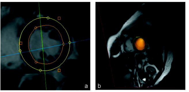
(a) Short axis MRI scan with superimposed epicardial (outer) and endocardial (inner) boundaries. (b) 3D surface created generated from the contours and superimposed on the short axis slice.

Quantification of Myocardial Wall Thickness

The definition of thickness as a metric must be carefully considered because the myocardium is a complex 3D structure with variable thickness. If thickness was defined as a straight-line distance between the two surfaces, this distance could be defined as the perpendicular projection between surfaces (as shown in Figure 2a) or as the minimum distance between surfaces as illustrated in Figure 2b. The problem with straight-line definitions is that, in cases where endocardial and epicardial surfaces are not parallel, wall thickness could be different depending on the surface from which the measurement is made (5, 28, 29, 30).

Figure 2.

Definition of thickness between surfaces S and S′. (a) Perpendicular projection from A to C, and B to A. (b) Minimum distance from A to B. (c) Thickness defined using Laplace’s equation (thickness lines) from A to B and C to D.

Laplace Method

To address the limitations of the straight-line approach, we borrowed tools from mathematical physics (30) to develop a new definition of thickness, one that was not based on a straight line principle. Our approach for myocardial thickness computation models the myocardial wall as a series of nested sub-layers bounded by the epicardial and endocardial surfaces, such as those shown in Figure 2(c). By integrating along the direction perpendicular to each sub-layer between the two surfaces, the thickness at any point in the wall is calculated. Every streamline could be associated with its length, and this could be used to define thickness (between C and D or A and B, in Figure 2c). The sublayers were modeled by assigning different boundary conditions to the two surfaces, and solving Laplace’s equation at each point between them.

Laplace’s equation is a second-order partial differential equation for a scalar field that is enclosed between boundaries S and S’. Mathematically, it takes the form:

$${\nabla }^2\mathrm{\Psi }=\frac{{\partial }^2\mathrm{\Psi }}{{\partial }^2{x}^2}+\frac{{\partial }^2\mathrm{\Psi }}{{\partial }^2{y}^2}+\frac{{\partial }^2\mathrm{\Psi }}{{\partial }^2{z}^2}$$ [1]

We solved Equation 1 iteratively throughout the entire data volume, keeping the boundaries fixed. Laplace’s equation was solved using the simplest Jacobi technique (31), which takes the following form:

$${\mathrm{\Psi }}_{i+1}(x,y,z)=[{\mathrm{\Psi }}_i(x+\mathrm{\Delta }x,y,z)+{\mathrm{\Psi }}_i(x-\mathrm{\Delta }x,y,z)+{\mathrm{\Psi }}_i(x,y+\mathrm{\Delta }y,z)+{\mathrm{\Psi }}_i(x,y-\mathrm{\Delta }y,z)+{\mathrm{\Psi }}_i(x,y,z+\mathrm{\Delta }z)+{\mathrm{\Psi }}_i(x,y,z-\mathrm{\Delta }z)]/6$$ [2]

Ψ_i represented the value at x, y, z when Laplace’s equation was solved during the ith iteration until convergence was achieved. Convergence was measured by the total field energy over all voxels, calculated by the equation:

$${\epsilon }_i=\sum {[{(\mathrm{\Delta }\mathrm{\Psi }i/\mathrm{\Delta }x)}^2+{(\mathrm{\Delta }\mathrm{\Psi }i/\mathrm{\Delta }y)}^2+{(\mathrm{\Delta }\mathrm{\Psi }i/\mathrm{\Delta }z)}^2]}^{\frac{1}{2}}$$ [3]

The resulting scalar field made a smooth transition, describing the nested sub-layers from one surface to another. Once the solution of Ψ was obtained, “field lines” were computed [4] and normalized [5].

$$\mathrm{E}=-\nabla \mathrm{\Psi }$$ [4]

$$\mathrm{N}=\mathrm{E}/\Vert \mathrm{E}\Vert$$ [5]

M represents a unit vector field, defined everywhere between S and S’, which always pointed perpendicular to the sublayer on which it was positioned. After computing M, “field lines” were computed by starting at any point on S and integrating M using finite differences derived from Taylor series expansions (32). Wall thickening (WT) was locally defined as increase in percentage thickness in terms of the wall thickness at ES, T_es and ED, T_ed respectively as shown in equation 6. We also implemented 2D Laplace to evaluate the error difference between the wall thickening measurements compared to the 3D technique.

$$\mathrm{WT}=({\mathrm{T}}_{\mathrm{es}}-{\mathrm{T}}_{\mathrm{ed}})/{\mathrm{T}}_{\mathrm{ed}}$$ [6]

EDT Method

We also compared the Laplacian technique for thickening with Euclidean distance transformation (EDT), a well known straight line based distance technique used in computer vision applied previously to cardiac MRI wall motion measurements (33). Danielson’s technique is a sequential algorithm, which provides an error-free computation of Euclidean distance mapping on a rectangular domain. This algorithm is based on propagation of vectors. Thus, it yields a vector map storing for each point of the horizontal and vertical distances from the closest reference point. The resulting 3D distance map assigns to each voxel of the volume the distance closest surface voxel. In short, the EDT of an N-dimensional binary image I is an N-dimensional image I_EDT such that for all indices i, element e_EDT,i ∈ I_EDT ⇒ e_EDT,i is the Euclidean distance from the element e_I,i to the nearest foreground element in I. We use ‘EDT_1’ to indicate the perpendicular projection from the epicardial to the endocardial surface and ‘EDT_2’ to indicate the projection from the endocardial to the epicardial surface.

Quantification of Myocardial Wall Motion

Regional myocardial motion measurements were obtained using EDT. To compute wall motion values, endocardial contours at ED were used as the reference. This is based on the observation that the maximum displacement of the myocardium during systole occurs in the endocardial layers. The distance map is a function of the perpendicular projection from the endocardial surface at ED to the endocardial surface at ES. The resulting distance map is the wall motion measurements in mm.

Implementation

The described algorithms were implemented in C++ on an Intel® Xeon® CPU Processor (3.00 GHz, 3.00 Gb RAM), and convergence occurred in less than 100 iterations for the data. Convergence was also achieved in less than 27 seconds per dataset.

Clinical and Experimental Testing

For regional assessment, the automatically obtained thickening and motion values were then mapped onto 2D polar map coordinates (Figures 3 and 4) by a projection of the volumetric data. Polar maps were subdivided according to the standard 17-segment model defined by the American Heart Association, containing 6 basal segments, 6 mid segments, 4 distal segments and 1 apical segment (34). Automatically obtained segmental measurements for wall motion and thickening were subsequently computed as averages of the polar map samples in these segments.

Figure 3.

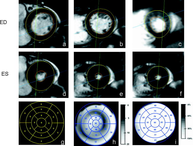
MRI scans and polar maps corresponding to a subject with summed visual score of 0. Short-axis MRI slices taken at ED at approximately the (a) basal-region, (b) mid-region, and (c) apical-region. The slices taken at ES corresponding to (d) basal, (e) mid and (f) apical-regions. The clinical scores on the 17-segment polar map (g), a grey-scale polar map of motion (h), and a thickening polar map (i) are also shown.

Figure 4.

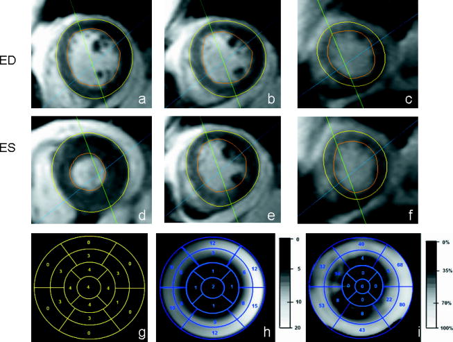
MRI scans and polar maps corresponding to a subject with summed visual score of 36. Short-axis MRI slices taken at ED, at approximately the (a) basal-region, (b) mid-region and (c) apical-region. The slices taken at ES corresponding to (d) basal, (e) mid and (f) apical-regions. The clinical scores on the 17 segment polar map (g), a grey-scale polar map of motion (h), and a thickening polar map (i) are also shown. The average thickening and wall motion of this subject was 25% and 6mm respectively.

Visual motion and thickening scoring

Two experienced imaging cardiologists (RN, BKT) recorded visual clinical scores twice within a month independently (4 readings in total). The readers were blinded to the automated data and the scoring was done using the 17-segment model with the standard 0-5 motion/thickening grading system (35). The observer’s scores were analyzed independently and also combined by averaging for wall measurement analysis. In clinical visual scoring, motion and thickening estimates were not separately assessed, and one overall score represented consideration of both endocardial motion and myocardial thickening. The visual grading system employed the following scores: 0 = normal wall thickening and motion, 1 = hypokinesis with mild decrease in wall thickening, 2 = hypokinesis with moderate decrease in wall thickening, 3 = hypokinesis with severe decrease in wall thickening, 4 = akinesis with no thickening, 5 = dyskinesis with no thickening. The sum of these scores provided a semiquantitative visual assessment of global ventricular dysfunction (36).

For global analysis from the computer-based analysis, mean thickening (in %) and mean motion (in mm) of the entire myocardium were computed from the polar map motion and thickening maps. Left ventricular ejection fraction (LVEF), end-diastolic (ED), and end-systolic (ES) volumes were derived from the same 3D ED and ES contours used to generate the thickening and motion maps (27).

Statistical analysis

Average quantitative thickening and motion measurements were compared with summed and regional visual scores using Spearman’s correlation. In addition, we use the Fisher z-transform to test whether two correlations have different strengths. P < 0.05 was considered significant.

Results

Figure 5a illustrates correlations between global measures of thickening/motion with EF. Correlation between LVEF and motion measurements was (r=0.86; p<0.0001) compared to the correlation between LVEF and thickening measurements (r=0.84; p<0.0001). In Figure 5b the relation of visual scores to quantitative thickening and motion measurements in the individual myocardial segments of the 53 patients is shown.

Figure 5.

Global and segmental analysis of wall thickening and motion. Global correlation of (a) average wall thickening and (b) average wall motion with EF. Segmental analysis of wall thickening (c) and motion (d) with visual clinical scores (all p<0.0001).

The two readers in our study had a substantial intra-observer agreement (κ = 0.67 with ~ 86% agreement). Linear weighted kappa revealed an intra-observer agreement of 96% as shown in Table 2. Inter-observer agreement between observers was (κ = 0.56) with 83 % agreement. A linear weighted kappa (κ = 0.78) with 95% inter-observer agreement was also obtained. In addition, the scores of the two independent observers were combined by averaging and a correlation value of -0.69 and -0.65 was obtained between the average scores and thickening/motion measurements respectively. Table 3 shows correlations for the visual and quantitative measurements in different myocardial regions. In addition, a correlation co-efficient of (r_thick = -0.79; r_motion= -0.74) was obtained between thickening/motion and summed combined visual scores respectively as presented in Table 4. Figure 6 compares the summed visual clinical scores with average quantitative percent thickening and average motion measurements. The bar graphs in Figure 6 demonstrate the inverse linear relationship between summed visual clinical score and average percent thickening/motion.

Table 2.

Intra- and inter- observer variation along with correlation statistics for segmental measurements and scores.

	Intra-variation	Read 1 vs measurements	Read 2 vs measurements
Observer1	K=0.67 (86% agreement) Weighted K=0.82 (96% agreement)	rthick = -0.71 rmotion = -0.68	rthick = -0.69 rmotion = -0.63
Observer2	K=0.67 (87% agreement) Weighted K=0.83 (96% agreement)	rthick = -0.57 rmotion = -0.60	rthick = -0.65 rmotion = -0.63
Combined Score		rthick = -0.69 rmotion = -0.65

Table 3.

Results of the regional analysis of thickening and motion.

	Thickening	Motion
Overall Correlation	(r=-0.69, p<0.0001)	(r=-0.65, p<0.0001)
Basal Regions	(r=-0.70, p<0.0001)	(r=-0.61, p<0.0001)
Mid Regions	(r=-0.68, p<0.0001)	(r=-0.69, p<0.0001)
Apical Regions	(r=-0.70, p<0.0001)	(r=-0.67, p<0.0001)

Table 4.

Results of the global analysis of thickening and motion.

	Thickening	Motion
LV Ejection Fractions	(r=0.84, p<0.0001)	(r=0.86, p<0.0001)
Summed Visual Score	(r=-0.79, p<0.0001)	(r=-0.74, p<0.0001)

Figure 6.

Summed visual clinical scores versus average quantitative (a) wall thickening and (b) motion in the 53 subjects studied.

LV ejection fraction (LVEF) ranged from 10% to 77% with a mean of 56±15%. The individuals with an LVEF >70% had small left ventricular size with end diastolic volumes between 35-50ml. We observed that these individuals exhibit hyperdynamic LV function during systole and this may therefore result in a higher than expected LV ejection fraction. The summed visual scores ranged from 0 to 55. Average global thickening and motion were found to be 61% and 9.7 mm, respectively. The dataset included twenty eight subjects with summed visual score of 0. In global analysis, correlation between LVEF and motion measurements was (r=0.86; p<0.0001) compared to the correlation between LVEF and thickening measurements (r=0.84; p<0.0001).

Examples of thickening and motion polar maps by visual scoring are displayed in Figure 3, a normal subject, and Figure 4, an abnormal subject. In the normal subject, wall thickness at end-systole (3(e)) was significantly greater than end-diastole (3(b)) in all segments. In the abnormal subject (summed visual score was 36), there was much less increase in wall thickness at end-systole.

For normal subjects (n=14), segmental analysis of thickening and motion are presented in the form of polar maps in Figure 7. Percent thickening increased from the basal to distal segments. Average thickening observed in the basal, mid, and distal segments were 60%, 79%, and 93% respectively. Wall motion, on the other hand, remained constant along the long axis (average motion: basal 11mm, mid 11mm, distal 10mm). Mean LVEF was 62±7% in these subjects. In addition, the 90^th percentile measurements for thickening and motion were computed and average segmental thickening and motion values were derived using the 17-segment model (Figure 7c and 7d). We observed that 94% of the segments (203/215) with visual scores > 0 were outside the 90^th percentile. For wall motion, (161/215) 75% of the segments with visual scores > 0 were outside the 90^th percentile.

Figure 7.

Segmental average (±standard deviation) of (a) thickening in % and (b) motion in mm of normal subjects. (c) contains 90^th percentile of thickening in % for normal subjects. (d) contains 90^th percentile of motion in mm for normal subjects.

We evaluated the performance of the Laplacian technique with EDT for thickening measurements using the coefficient of variation (standard deviation expressed as a percentage of the mean). The coefficient of variation is a useful measure to indicate whether each measurement technique is sensitive to small local segmentation errors [28-30]. The Laplacian technique resulted in lower coefficients of variation compared to ‘EDT_1’ and ‘EDT_2’. The average coefficient of variation among basal, mid and distal regions for Laplace was 56, 60 and 66%. The average coefficient of variation among the basal, mid and distal regions for ‘EDT_1’ and ‘EDT_2’ were 62, 62, 70% and 61, 65, 71% respectively. These results can be attributed to the potential limitations of straight line distance techniques. When 2D and 3D Laplace methods were compared, the absolute sum difference between the two techniques for basal, mid and apical regions were 19%, 13% and 7% respectively.

Discussion

Previous studies have presented quantitative wall thickening/motion techniques based on volume element approaches, which, in some cases, required additional tagged MR imaging acquisitions (17-19). Volume element techniques (20, 21) partition the myocardium into large volumetric segments. Average wall thickness is then derived for each element from its volume and geometric assumptions about its shape. The limitations of this approach include a relatively small number of segments along the circumference of the myocardium, creation of volume elements in between image slices, and assumptions regarding left ventricular shape. The use of MR tagging to assess wall thickening is limited by poor spatial resolution if an insufficient number of tags are used (17-19). Also, when tag lines are oriented in parallel in long axis images, apical motion may be excluded. Van der Geest et al (10) and Holman et al. (11) have proposed a 3D technique based on a straightforward extension of the 2D centerline method. More recently, Beohar et al. analyzed regional LV function with cardiac MRI after myocardial infarction using a very similar approach (13). However, these techniques are inherently straight-line based, and thus can be sensitive to imperfect contours. Several studies have also used the centerline technique and its improved version to evaluate wall motion, wall thickness, and wall thickening at 100 points or chords around the LV wall (9, 11, 12, 14).

In this work, we developed and clinically validated fully 3D regional quantification of wall thickening and motion. Results could be presented in a 17-segment model format and compared with visual scoring. Good correlation was observed between motion/thickening and clinical visual scores. In addition, we established quantitative normal ranges for segmental wall thickening and motion based on data identified by experts as normal based on medical records, which has not been previously reported.

Our approach models the myocardial wall as a series of nested sub-layers bound by epicardial and endocardial surfaces. The thickness at any point in the wall is calculated by integrating along the direction perpendicular to each sub-layer between the two surfaces. Hence, it is a requirement for the region defined between the epicardium and endocardium to be available. Conceivably, motion could be represented as a Laplace problem by using the concept of abstract “thickness” between ED and ES endocardium to calculate the excursion of the endocardium. However, when computing motion of the endocardial surface between the end-systolic and end-diastolic phases, it is difficult to obtain a well defined contiguous region, limiting the utility of Laplace’s equation in calculating motion; therefore alternative EDT approach was used for computation of motion.

The global measures were computed by averaging the wall measurements across the whole myocardium. Among the cases with high EFs (>50%), certain segments thickened differently compared to the remaining segments in different regions. Also, a normal myocardium has varying degrees of thickening across different regions, which is reflected in Figure 5(c). The global analysis incorporates average thickening of the whole myocardium, which could potentially result in higher variation in the thickening measurements.

Approximately, 5 minutes per phase for each case were spent by the medical experts in adjusting contours to exclude papillary muscles and trabeculations. This is still considerably less time spent by the experts when compared to fully manual contouring of the cardiac cases. The Laplacian technique, on average, took 23 ± 3.7 seconds to produce the thickening measurements using the volumetric dataset over two phases. The wall motion technique, on the other hand, took an average of 13 ± 3.9 seconds to produce motion measurements.

For normal subjects, we found that the average wall motion remained constant along the long axis as demonstrated for SPECT by Sharir et al. (36). Average wall thickening, on the other hand, increased from basal (60±11%) to distal (93±12%) along the long axis, confirming data previously reported by others (37, 38). This finding may be explained by the presence of the LV outflow tract (LVOT), which occupies a portion of the LV base and contains fibrous tissue that does not normally thicken. Readers can account for this by visually excluding the LVOT when assessing myocardial wall thickening.

Limitations

The reference standard, against which our automatic quantitative regional function analysis was tested, was expert visual assessment of regional wall motion and wall thickening, which represents current clinical practice. It is important to note that the visual scoring system is a qualitative technique associated with intra- and inter-observer variability. This could explain some of the discrepancies in the results. Additionally, discrepancies may have occurred due to the discrete scale of user grading, as reflected in the correlation values for segmental analysis. However, this effect was reduced when summed visual clinical scores are used, resulting in strong correlation values for global analysis.

The goal of this study is to develop regional analysis technique which can be applied to standard clinical data. The number of slices and slice thickness is indeed technically limited by practical considerations such as the total length of the scan, noise level and the time required for one breath-hold. Our technique used ED and ES myocardial 3D contours only. Abnormal wall motion in other phases of the cardiac cycle or abnormal diatolic function is therefore not detected. Our technique quantified wall thickening and wall motion separately; however, visual clinical score is a combined score of wall thickening and motion; however this reflects the current standard clinical practice. Additionally, the visual scores are categorical in nature. One way to potentially improve the reported results would be to merge the quantitative thickening and motion polar maps into a combined motion/thickening score.

The apical regions reflect poor contrast and increase in curvature where the contours are approximated by the experts, resulting in rapid changes in the contour boundaries. Since Laplace uses the boundaries to model the myocardium as a series of nested sub-layers, potentially these rapid changes will impact the shape of the sub-layers. The algorithm was not optimized for performance and although, it may appear as a limiting factor, this is still a significant gain when an expert would need to compute thickening or motion manually. The experts, when timed took on average 7 minutes to visually score each case.

When identifying normal subjects to establish normal limits, we did not stratify based on age or gender due to limited number of studies available for this analysis. These variables may play a very important role with respect to LV chamber size wall thickness and ventricular relaxation parameters. This would necessitate obtaining a larger group of normal controls.

In conclusion, we have developed a novel technique based on Laplace’s equation to compute regional 3D myocardial thickening over the entire left ventricle using MRI and established quantitative normal ranges for segmental thickening/motion visually considered as normal. Our algorithm generated wall motion and thickening values that exhibited strong global and regional correlation with LVEF and clinical visual scoring, and should be considered a step towards accurate quantitative assessment of the regional myocardial function from cardiac MRI.

References

- 1.Sakuma H, Fujia N, Foo TKF, et al. Evaluation of left ventricular volume and mass with breath-hold cine MR imaging. Radiology. 1993;188:377–380. doi: 10.1148/radiology.188.2.8327681. [DOI] [PubMed] [Google Scholar]
- 2.Young AA, Kramer CM, Ferrari VA, Axel L, Reichek N. Three dimensional left ventricular deformation in hypertrophic cardiomyopathy. Circulation. 1994;90:854–867. doi: 10.1161/01.cir.90.2.854. [DOI] [PubMed] [Google Scholar]
- 3.Epstein FH. MRI of left ventricular function. J Nuclear Cardiology. 2007;14(5):729–744. doi: 10.1016/j.nuclcard.2007.07.006. [DOI] [PubMed] [Google Scholar]
- 4.Haag UJ, Maier SE, Jakob M, et al. Left ventricular wall thickness measurements by magnetic resonance: a validation study. Int J Cardiac Imag. 1991;7:31–41. doi: 10.1007/BF01797678. [DOI] [PubMed] [Google Scholar]
- 5.Van Rugge FP, Van der Wall EE, Spanjersberg SJ, et al. Magnetic resonance imaging during dobutamine stress for detection of coronary artery disease; quantitative wall motion analysis using a modification of the centerline method. Circulation. 1994;90:127–138. doi: 10.1161/01.cir.90.1.127. [DOI] [PubMed] [Google Scholar]
- 6.Holman ER, Vliegen HW, Van der Geest RJ, et al. Quantitative analysis of regional left ventricular function after myocardial infarction in the pig assessed with cine magnetic resonance imaging. Magn Reson Med. 1995;34:161–169. doi: 10.1002/mrm.1910340206. [DOI] [PubMed] [Google Scholar]
- 7.Baer FM, Smolarz K, Theissen P, Voth E, Schicha H, Sechtem U. Regional 99mTc-methoxyisobutyl-isonitrile-uptake at rest in patients with myocardial infarcts: comparison with morphological and functional parameters obtained from gradient-echo magnetic resonance imaging. Eur Heart J. 1994;15:97–107. doi: 10.1093/oxfordjournals.eurheartj.a060386. [DOI] [PubMed] [Google Scholar]
- 8.Azhari H, Sideman S, Weiss JL, et al. Three-dimensional mapping of acute ischemic regions using MRI: wall thickening versus motion analysis. Am J Physiol. 1990;259:H1492–H503. doi: 10.1152/ajpheart.1990.259.5.H1492. [DOI] [PubMed] [Google Scholar]
- 9.Von Land CD, Rao SR, Reiber JHC. Development of an improved centerline wall motion model. Comput Cardiol. 1990:687–690. [Google Scholar]
- 10.van der Geest RJ, de Roos A, van der Wall EE, Reiber JHC. Quantitative analysis of cardiovascular MR images. The International Journal of Cardiac Imaging. 1997;13:247–258. doi: 10.1023/a:1005869509149. [DOI] [PubMed] [Google Scholar]
- 11.Holman ER, Buller VG, de Roos A, et al. Detection and Quantification of Dysfunctional Myocardium by Magnetic Resonance Imaging. A New Three-dimensional Method for Quantitative Wall-Thickening Analysis. Circulation. 1997;95:924–931. doi: 10.1161/01.cir.95.4.924. [DOI] [PubMed] [Google Scholar]
- 12.Buller VGM, van der Geest RJ, Kool MD, Reiber JHC. Accurate three-dimensional wall thickness measurement from multi-slice short-axis MR imaging. Proceedings of Computers in Cardiology; Vienna, Austria. 1995; pp. 245–248. [Google Scholar]
- 13.Beohar N, Flaherty JD, Davidson CJ, Vidovich MI, Brodsky A, Lee DC. Quantitative assessment of regional left ventricular function with cardiac MRI: Three-dimensional centersurface method. Catheter Cardiovasc Interv. 2007;69:721–728. doi: 10.1002/ccd.21048. [DOI] [PubMed] [Google Scholar]
- 14.Sheehan FH, Bolson EL, Dodge HT, Mathey DG, Schofer J, Woo HK. Advantages and applications of the centerline method for characterizing regional ventricular function. Circulation. 1986;74:293–305. doi: 10.1161/01.cir.74.2.293. [DOI] [PubMed] [Google Scholar]
- 15.Saeed M, Wendland MF, Yu KK, et al. Identification of myocardial perfusion with echo planar magnetic resonance imaging; discrimination between occlusive and reperfused infarctions. Circulation. 1994;90:1492–1501. doi: 10.1161/01.cir.90.3.1492. [DOI] [PubMed] [Google Scholar]
- 16.Saeed M, Wendland MF, Szolar D, et al. Quantification of extent of area at risk with fast contrast-enhanced magnetic resonance imaging in experimental coronary artery stenosis. Am Heart J. 1996;132:921–932. doi: 10.1016/s0002-8703(96)90000-9. [DOI] [PubMed] [Google Scholar]
- 17.Maier SE, Fischer SE, McKinnon GC, Hess OM, Krayenbuehl HP, Boesiger P. Evaluation of left ventricular segmental wall motion in hypertrophic cardiomyopathy with myocardial tagging. Circulation. 1992;86:1919–1928. doi: 10.1161/01.cir.86.6.1919. [DOI] [PubMed] [Google Scholar]
- 18.Lima JA, Jeremy R, Guier W, et al. Accurate systolic wall thickening by NMR imaging with tissue tagging: correlation with sonomicrometers in normal and ischemic myocardium. J Am Coll Cardiol. 1993;21:1741–1751. doi: 10.1016/0735-1097(93)90397-j. [DOI] [PubMed] [Google Scholar]
- 19.Dong SJ, MacGregor JH, Crawley AP, et al. Left ventricular wall thickness and regional systolic function in patient with hypertrophic cardiomyopathy. A three-dimensional tagged magnetic resonance imaging study. Circulation. 1994;90:1200–1209. doi: 10.1161/01.cir.90.3.1200. [DOI] [PMC free article] [PubMed] [Google Scholar]
- 20.Beyar R, Shapiro EA, Graves WL, et al. Quantification and validation of left ventricular wall thickening by a three-dimensional volume element magnetic resonance imaging approach. Circulation. 1990;81:297–307. doi: 10.1161/01.cir.81.1.297. [DOI] [PubMed] [Google Scholar]
- 21.Beyar R, Weiss JL, Shapiro EP, Graves WL, Rogers WJ, Weisfeldt ML. Small apex-to-base heterogeneity in radius-to-thickness ratio by three-dimensional magnetic resonance imaging. Am J Physiol. 1993;264:H133–H40. doi: 10.1152/ajpheart.1993.264.1.H133. [DOI] [PubMed] [Google Scholar]
- 22.Barest GD, Bacharach SL, Douglas MA, et al. Myocardial wall thickness and thickening from gated magnetic resonance images. Proceedings of Computers in Cardiology; Los Alamitos. 1991; pp. 629–632. [Google Scholar]
- 23.Pujadas S, Reddy GP, Weber O, Lee JJ, Higgins CB. MR Imaging Assessment of Cardiac Function. Journal of Magnetic Resonance Imaging. 2004;19:789–799. doi: 10.1002/jmri.20079. [DOI] [PubMed] [Google Scholar]
- 24.Diamond GA, Staniloff HM, Forrester JS, Pollock BH, Swan HJ. Computer-assisted diagnosis in the noninvasive evaluation of patients with suspected coronary artery disease. J Am Coll Cardiol. 1983;1:444–455. doi: 10.1016/s0735-1097(83)80072-2. [DOI] [PubMed] [Google Scholar]
- 25.Bloomer TN, Plein S, Radjenovic A, et al. Cine MRI using steady state free precession in the radial long axis orientation is a fast accurate method for obtaining volumetric data of the left ventricle. J Magn Reson Imaging. 2001;14:685–692. doi: 10.1002/jmri.10019. [DOI] [PubMed] [Google Scholar]
- 26.Slomka P, Fieno D, Ramesh A, et al. Patient motion correction for multiplanar, multi-breath-hold cardiac cine MR imaging. J Magn Reson Imaging. 2007;25:965–973. doi: 10.1002/jmri.20909. [DOI] [PubMed] [Google Scholar]
- 27.Slomka P, Mehta T, Aladl UE, Berman DS, Germano G. A fully automated registration-based technique for segmentation of the left ventricle from cardiac MRI. Proceedings of the 8th Annual Meeting of ISMRM; Japan. 2004; abstract 1803. [Google Scholar]
- 28.Prasad M, Brown MS, Ni C, et al. Three-dimensional mapping of gallbladder wall thickness on CT using Laplace’s equation. Academic Radiology. 2008;15:1075–1081. doi: 10.1016/j.acra.2008.02.006. [DOI] [PubMed] [Google Scholar]
- 29.Prasad MN, Brown MS, Ni C, et al. Reproducibility of Laplacian wall thickness measurements of the gallbladder with varying CT slice thickness. Journal of Signal Processing Systems. 2008 doi: 10.1007/s11265-008-0199-1. [DOI] [Google Scholar]
- 30.Jones SE, Buchbinder BR, Aharon I. 3D mapping of cortical thickness using Laplace’s equation. Human Brain Mapping. 2000;11:12–32. doi: 10.1002/1097-0193(200009)11:1<12::AID-HBM20>3.0.CO;2-K. [DOI] [PMC free article] [PubMed] [Google Scholar]
- 31.William SA, Press H, Flannery BP, Vetterling WT. Numerical recipes in C: The art of scientific computing. Cambridge: Cambridge University Press; 1993. p. 1035. [Google Scholar]
- 32.DuChateau P, Zachmann D. Applied partial differential equations. New York: Harper and Row; 1989. p. 640. [Google Scholar]
- 33.Danielson PE. Euclidean distance mapping. Computer Graphics and Image Processing. 1980;14:227–248. [Google Scholar]
- 34.Cerqueira MD, Weissman NJ, Dilsizian V. Standardized myocardial segmentation and nomenclature for tomographic imaging of the heart. Circulation. 2002;105:539–542. doi: 10.1161/hc0402.102975. [DOI] [PubMed] [Google Scholar]
- 35.Cooke CD, Garcia EV, Cullom SJ, Faber TL, Pettigrew RI. Determining the accuracy of calculating systolic wall thickening using a fast Fourier transform approximation: a simulation study based on canine and patient data. J Nucl Med. 1994;35:1185–1192. [PubMed] [Google Scholar]
- 36.Sharir T, Berman DS, Waechter PB, et al. Quantitative analysis of regional motion and thickening by gated myocardial perfusion SPECT: normal heterogeneity and criteria for abnormality. J Nucl Med. 2001;42:1630–1638. [PubMed] [Google Scholar]
- 37.Ordas S, Frangi AF. Automatic quantitative analysis of myocardial wall motion and thickening from long- and short-axis cine mri studies. Proceedings of the 27th Annual International Conference of the IEEE Engineering in Medicine and Biology Society (EMBS); China. 2005; 1991. pp. 7028–7031. [DOI] [PubMed] [Google Scholar]
- 38.Germano G, Erel J, Lewin H, Kavanagh PB, Berman DS. Automatic quantitation of regional myocardial wall motion and thickening from gated technetium-99m sestamibi myocardial perfusion single-photon emission computed tomography. J Am Coll Cardiol. 1997;30:1360–1367. doi: 10.1016/s0735-1097(97)00276-3. [DOI] [PubMed] [Google Scholar]