A nonparametric approach to detect nonlinear correlation in gene expression

Abstract

We propose a distribution-free approach to detect nonlinear relationships by reporting local correlation. The effect of our proposed method is analogous to piece-wise linear approximation although the method does not utilize any linear dependency. The proposed metric, maximum local correlation, was applied to both simulated cases and expression microarray data comparing the rd mouse with age-matched control animals. The rd mouse is an animal model (with a mutation for the gene Pde6b) for photoreceptor degeneration. Using simulated data, we show that maximum local correlation detects nonlinear association, which could not be detected using other correlation measures. In the microarray study, our proposed method detects nonlinear association between the expression levels of different genes, which could not be detected using the conventional linear methods. The simulation dataset, microarray expression data, and the Nonparametric Nonlinear Correlation (NNC) software library, implemented in Matlab, are included as part of the online supplemental materials.

1 Introduction

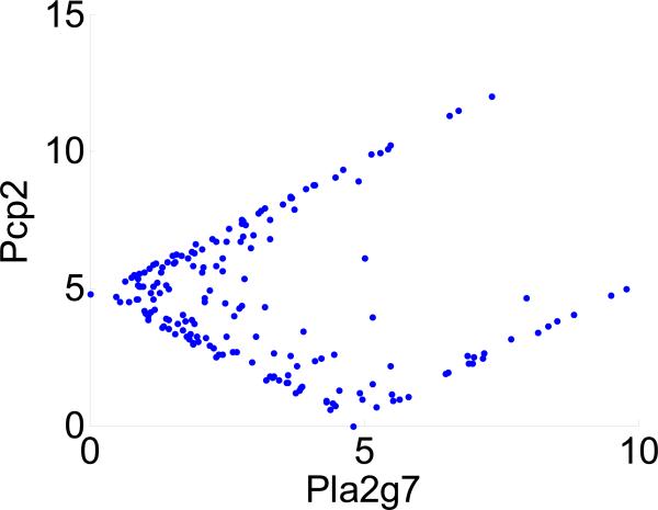
Although nonlinear relationships between the expression levels of genes or gene products are expected (Kitano, 2002a,b) and observed (Rohrer et al., 2004) in biological datasets, there is no commonly used statistic quantifying nonlinear correlation that can find a similarly generic use as Pearson's correlation coefficient for quantifying linear correlation. Many analyses of complex biological phenomena still approach the biological question of correlation using global linear association only. Mutual information has been used to detect nonlinear correlation in microarray expression dataset, implicitly (Kasturi and Acharya, 2005) and explicitly (Steuer et al., 2002; Daub et al., 2004). However, different estimation methods of the mutual information lead to different conclusions. We propose a method to quantify global nonlinear relationship by reporting local correlation. Local here refers to the correlation that exists either at a certain scale or under certain condition(s), and is therefore also referred to as transient correlation. An example is illustrated in Figure 1 that includes partial signals that are positively correlated and partial signals that are negatively correlated. However, neither linear dependency is assumed nor used in our method. That is, the association need not be linear to be detected at either the local or global scale. Our proposed method quantifies correlation by examination of bivariate distances between data points and was inspired by the use of the correlation integral in a fluctuating dynamic system (Grassberger and Procaccia, 1983).

Figure 1.

An example of nonlinear correlation observed in the microarray study (in Section 4). Nonlinear correlation can be detected by maximal local correlation (M = 0.93, p = 0.007), but not by Pearson correlation (C = –0.08, p = 0.88) between genes Pla2g7 and Pcp2 (i.e., between two columns of the distance matrix). Pla2g7 and Pcp2 are negatively correlated when their transformed levels are both less than 5. These two genes are, otherwise, positively correlated. More experimental and data processing details are provided in Section 4.

The correlation integral examines the cumulative distribution of distances between data points of a time series. With proper modification, we show that the correlation integral can be used to estimate global patterns and global association. We develop statistics using the correlation integral to estimate local correlation. We only focus on bivariate correlation.

The need for quantification of nonlinear relationships is particularly acute for expression microarray data, where a massive number of variables and a wide range of biological processes involved in a typical experiment represent a particularly convoluted version of the proverbial “search for a needle in a haystack”. Aside from the nonlinearity, several additional challenges (Quackenbush, 2001) are commonly found in high-throughput biological datasets: 1) different datasets have different scales, 2) the scale that is potentially biologically relevant is often unknown at the exploratory stage of the research, 3) high noise levels (Marshall, 2004), and 4) the sampling distribution is generally unknown, very seldom if ever is the data normally distributed. Multi-modality is not uncommon. We propose a generic method to quantify nonlinear correlation by reporting local correlation, with the option of removal of the scaling effects between different measurements, which will 1) detect association at multiple scales, 2) be insensitive to noise, and 3) not rely on distribution assumptions, i.e., a nonparametric method.

In Section 2, the correlation integral is introduced and we define the proposed measures of local correlation and of correlation change. Local correlation measures are used to describe the relationships across experimental units, genes in the case of our motivating application. On the other hand, correlation change allows us to identify experimental units whose relationships differ across two conditions, in our case gene expression in a treatment group versus a control group. In Section 3 we validate our method on simulated cases. Finally, in Section 4, we use the proposed measures to quantify nonlinear association change in microarray expression between a treatment group and a control group in an animal experiment. The treatment group are mice exhibiting photoreceptor degeneration (rd) and the control group are wild type mice (wt). The rd mouse is also referred to as the rd1 mouse in the literature. The generality of the proposed method makes it appropriate to many other types of data, such as those generated by proteomics or metabolomics.

2 Local Correlation

We first describe the proposed summary of bivariate local correlation in words. Formal definition of the proposed method and the notations will follow in the next few paragraphs. First, each variable is transformed such that the marginal distribution is uniform. This is achieved by transforming to ranks (in ascending order) followed by a linear transformation. Let N denote the sample size. The linear transformation is achieved by subtracting the minimum rank (i.e., 1, in the absence of ties) from the ranks and then divided by the difference between maximum rank and minimum rank (i.e., N – 1, in the absence of ties). The rank transformation is the default setting in our implementation. Alternatively, this preprocessing step can be omitted if the raw data are already on comparable and non-arbitrary scales. Next we evaluate the neighbor density, which records the rate of change of the number of observations within a neighborhood of a given radius. We then compare the observed neighbor density with the neighbor density under the null hypothesis of no linear or nonlinear association. The difference defines the proposed measure of local correlation. Finally, we define maximum local correlation to describe overall bivariate nonlinear correlation.

The definition of the proposed method is based on the concept of correlation integrals. Consider a time series, z_i, i = 1, . . . , N. The correlation integral I(r) is defined as (Grass-berger and Procaccia, 1983):

$$I\left(r\right)=\underset{N\to \infty }{\text{lim}}\left\{\frac{1}{N^2}\sum _{i,j=1}^{N}I(\mid z_i-z_j\mid <r)\right\}$$

The correlation integral quantifies the average cumulative number of neighbors within radius r. The definition remains meaningful also when the data are not a time series.

To develop a measure of association between vectors, x and y, we modify the definition of I(r) as follows. Let z_i = (x_i, y_i), i = 1, . . . , N, denote the observations in the dataset and let |z_i – z_j| denote Euclidean distance. We define $\widehat{I}\left(r\right)<\frac{1}{N^2}{\sum }_{i,j=1}^{N}I(\mid z_i-z_j\mid =r)$. The observed distances are further linearly transformed between 0 and 1 before quantifying Î. Note that Î has the property of a cumulative distribution function (cdf). It is nondecreasing from 0 to 1 and continuous from the right. The function Î(r) describes the global pattern of neighboring distances.

Our primary interest is the definition of a metric to quantify nonlinear association by reporting local patterns. Therefore the neighbor density D is devised as the derivative of Î:

$$\widehat{D}\left(r\right)=\Delta \widehat{I}\left(r\right)∕\Delta r$$

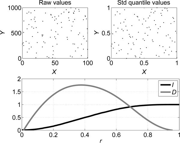
where ΔÎ(r) denotes change in Î(r). The observed neighbor density is evaluated at the discrete radius r, where r = 0, 1/m, 2/m, . . . , 1, and m is an arbitrary grid size that determines Δr = 1/m. An automatic smoother using cross-validation to choose an optimal window size (Vilela et al., 2007) is applied to smooth $\widehat{D}\left(r\right)$. Any traditional smoothing algorithms with proper choice of smoothing window size could alternatively be used here. In our study, the default size m is set as N, the number of observations. The statistic $\widehat{D}$ is a discrete approximation of dÎ(r)/dr, which has the formal properties of a probability density function (pdf). Therefore, with a slight abuse of terminology we refer to $\widehat{D}\left(r\right)$ as a distribution. An example of a correlation integral and a neighbor density is illustrated in Fig. 2.

Figure 2.

An example of the correlation integral (Î) and neighbor density $\left(\widehat{D}\right)$ for a null distribution i.e., in the absence of correlation between x and y.

Local correlation $\left(\ell \right)$

Intuitively, the distances between data points between two correlated variables would differ from that between two uncorrelated variables. Let ${\widehat{D}}_o\left(r\right)$ denote the estimate of a null distribution, which is composed of two vectors without any bassociation. We define local correlation $\left(\ell \right)$ as the deviation of $\widehat{D}$ from that of the null distribution at a given neighboring distance r:

$$\ell \left(r\right)=\widehat{D}\left(r\right)-{\widehat{D}}_o\left(r\right)$$ (1)

Our approach does not assume any parametric distribution. The flexibility of this method makes it easy to change the null distribution to any distribution of interest. The null hypothesis H_o of no difference between the observed neighbor density $\widehat{D}$ and ${\widehat{D}}_0$ is $H_o:\ell \left(r\right)=0$ for r = 0, 1/m, . . . , 1. Let $z^{\star }\left(b\right)$, b = 1, 2, . . . , B, denote permutation replicates (see Appendix A for details) and let ${\ell }^{\star }(r,b)$ be corresponding permutation evaluations of $\ell \left(r\right)$. A two-sided p-value can be evaluated by (Efron and Tibshirani, 1993):

$$p(\ell ,r)=\#\{\mid {\ell }^{\star }(r,b)\mid >\mid \ell \left(r\right)\mid \}∕B$$ (2)

where r = 0, 1/m, . . . , 1. Multiplicity correction could be carried out to adjust for the m tests performed. This could be done through the control of either false discovery rate (FDR) or experiment-wide error. In the following sections, we make use of these two alternative approaches for different aspects of the inferences.

Maximal local correlation (M)

Local correlation is further used for the definition of a summary statistic, maximum local correlation M, to describe overall nonlinear association. Using an idea similar to the Kolmogorov-Smirnov statistic, maximum local correlation is defined, as its name implies, by

$$M=\underset{r}{\text{max}}\left\{\mid \ell \left(r\right)\mid \right\}.$$

The interpretation of $\ell \left(r\right)$ as the difference of two pdf's implies that M can be interpreted as distance under the supremum norm of D and D_o. In other words, we define the statistic M as the maximum deviation between two underlying neighbor densities. Statistical significance of M is assessed in a permutation procedure similar to (2). See Appendix B for details.

Correlation change (δ_M)

Recall that the motivating application for the development of the local correlation measures ℓ and M is an application for microarray data analysis. We will report details of the experiment and the data later, in Section 4. The setup is such that local correlation between responses for gene i and responses for gene j can be interpreted as measuring the relationship between genes i and j. Like many microarray experiments, the data includes measurements under two biologic conditions, wt and rd. The ultimate inference goal is to understand how the two different biologic conditions affect the gene functions. We formalize this inference goal by considering the change in local correlation between the two conditions.

Building upon maximal local correlation M, we propose a statistic δ_M to measure association change. The motivation is that nonlinear behavior in biology can reflect the fact that the molecular machinery that is underlying biological processes is reconfigured to changes occurring in physiological or diseased states. In the microarray data example, for each pair of genes (ij) we want to test whether there is a change of nonlinear correlation between rd and wt mice. We therefore define a statistic δ_M to identify changes in maximal local correlation. We will later use it to identify critical genes in the disease development process. The statistic δ_M is defined as

$${\delta }_M=M^{rd}-M^{wt}$$ (3)

The results using our proposed methods are compared to those obtained using existing methods, including Pearson's linear correlation (C), Spearman's rank correlation coefficient, and mutual information (MI) as a nonlinear approach. Mutual information is evaluated using the R function mutual_information2() (Daub et al., 2004). The default setting was used for the R function. See Appendix C for a definition of MI. MI is a summary of (nonlinear) association between x and y. We use it for a comparison of various performance summaries in the examples. No details are needed for the upcoming discussion. See Daub et al. (2004) for more details.

The statistical significance for C and MI is estimated using the same permutation procedures as for M to ensure comparability. See (A.1) and (A.2) in Appendix A. Similar to (3) we define

$${\delta }_S=S^{rd}-S^{wt}\text{where}S=M,C,MI.$$ (4)

Permuatation tests for δ_S are defined in (B.1) in Appendix B.

3 Simulation Study

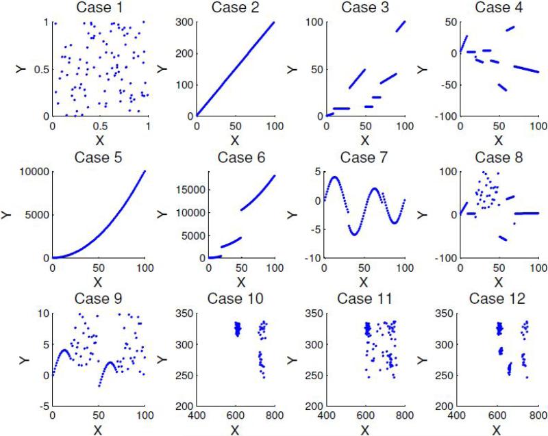
Twelve cases representing linear or different non-linear relationships were considered (Fig. 3). Case 1 is composed of independent vectors x and y. The observations of x and y in Case 2 have a perfect linear relationship. Case 3 is composed of 7 non-decreasing broken straight lines while Case 4 has 8 broken straight lines. Case 5 is a continuous monotonically increasing curve and Case 6 has 3 broken monotonically increasing curves; Case 7 is composed of three segments of sine waves. Case 8 is a mixture distribution of Cases 1 and 4 while Case 9 is a mixture of Cases 1 and 7. The 3 clusters in Case 10 are randomly sampled 100 data points from dataset 1 from Jonnalagadda and Srinivasan (2004). Case 11 is a mixture distribution of Cases 10 and 1, that is, a mixture of 3 clusters along with some background noise. Two-fifths of the data points in Case 11 are randomly sampled from Case 1 while 3/5 of the data are randomly sampled from Case 10. Case 12 includes five clusters with 3/5 of the data points randomly sampled from Case 10 and the remaining 2/5 of additional clusters (Fig. 3). The dataset (Jonnalagadda and Srinivasan, 2004) and the Matlab scripts to generate the simulated cases are included as supplemental materials. We evaluate ℓ and M for each case. For each case with stochastic components, i.e., Cases 1 and 8 through 12, we simulated 100 realizations to estimate positive rates of testing for significant maximum local correlation M under repeat simulation. For Case 1 the (false) positive rate is a type I error. For cases 8 through 12 the (true) positive rate is interpreted as statistical power. The results are summarized in Table 1. Maximum local correlation M was computed for the raw data values, without rank transformation, to keep results comparable with other correlation methods (Pearson's correlation, Spearman's correlation, and mutual information, which will be described later).

Figure 3.

Twelve simulated cases. 1) random points; 2) a straight line; 3) broken nondecreasing straight lines; 4) broken straight lines; 5) a continuous monotonically increasing curve; 6) broken monotonically increasing curves; 7) three partial sine waves; 8) a mixture distribution of Cases 1 and 4; 9) a mixture distribution of Cases 1 and 7; 10) three clusters; 11) a mixture distribution of Cases 10 and 1; 12) five clusters.

Table 1.

Comparison of local and global correlations. Listed are positive rates for Cases 1, 8 to 12, and correlation measurement (with estimated p-value) for Cases 2 to 7. For Case 1 the (false) positive rate is type-I error. For Cases 8 through 12 the (correct) positive rate is statistical power.

Case	M	MI	C	Sp
positive rates
1	3 %	1%	3 %	3 %
8	100 %	100 %	96 %	3 %
9	100 %	100 %	22 %	11 %
10	100 %	100 %	100 %	99 %
11	100 %	99 %	100 %	98 %
12	100 %	100 %	98 %	100 %
Correlation measurement (p-values)
2	1.60 (< ε)	3.32 (< ε)	1.00 (< ε)	1.00 (< ε)
3	1.55 (< ε)	2.01 (< ε)	0.76 (< ε)	0.82 (< ε)
4	1.47 (< ε)	2.14 (< ε)	−0.40 (< ε)	−0.59 (< ε)
5	0.08 (< ε)	2.39 (< ε)	0.97 (< ε)	1.00 (< ε)
6	0.19 (0.0005)	2.60 (< ε)	0.97 (< ε)	1.00 (< ε)
7	1.60 (< ε)	1.67 (< ε)	−0.37 (< ε)	−0.40 (< ε)

ε = 2.50 · 10^–4. For the cases with stochastic components, i.e., Cases 1, and 8 to 12, the estimated positive rate is listed based on 100 simulations for each case. M: maximum local correlation; MI: mutual information; C: Pearson correlation; Sp: Spearman correlation.

Local correlation $\left(\ell \right)$

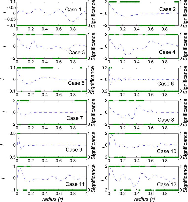
Fig. 4 shows the local correlations $\ell \left(r\right)$ from one simulation for each of the 12 cases. Significant local correlations were found in all simulated cases, except (correctly) for Case 1. Here, significance is determined after a Bonferroni correction $(p(\ell ,r)\le 5\cdot {10}^{-4})$.

Figure 4.

Local correlation between x and y for one simulated dataset from each of the 12 simulated cases. The dashed curves are the estimated local correlations $\left(\ell \left(r\right)\right)$ (using the y-axis on the left). The solid dots indicate the statistical significance of local correlations (using the y-axis on the right). It is labeled as 1 if local correlation is significant after Bonferroni correction, 0 otherwise. Local correlations (and the associated significance) are plotted against the radius (r).

Positive local correlation means that the observed neighbor density is greater than the neighbor density under the null hypothesis when evaluated at radius r. Negative local correlation means that the observed neighbor density is lower than the neighbor density under the null hypothesis. Significant local correlations are detected at almost all scales (of radius r) in Case 2, which is a boundary condition with perfectly linear relationship. The profile of ℓ peaks near 0 and decreases along r. Observed multi-modal $\ell \left(r\right)$ for all cases except Case 1 showed significant correlation at multiple scales. Statistically significant local correlation was observed for Case 11 although it contains both, the signals of Case 10 and the noise from Case 1.

Maximal local correlation (M)

Maximal local correlation is a summary statistic to test global nonlinearity while ℓ reports local correlation as a function of the neighborhood width of interest r. All cases with only deterministic components, i.e., Cases 2 to 7, had statistically significant maximum local correlation M at significance level α = 0.05 (Table 1). The stochastic component in the remaining Cases 1 and 8 through 12 allows us to evaluate positive rates across repeat experimentation. Except for Case 1, we (correctly) detect significant maximal local correlation for all 100 repeat simulations performed for each of these cases. That is, 100% true positive rates for Cases 8 through 12. Positive rate for these cases is interpreted as power. The (false) positive rate for maximal local correlation for Case 1 is 3% (Table 1). It is interpreted as type I error.

Comparison with other correlation coefficients

Pearson's (C), Spearman's (Sp), maximum local correlation (M), and mutual information (MI) for the 12 simulated cases are compared in Table 1. The results of Pearson's and Spearman's correlations showed that the majority of cases have significant global linear correlation, i.e., downward or upward trends, except for Case 1. When the global up or downward trend is weak, i.e., Cases 8 and 9, the statistical power for Pearson and Spearman's correlation is lower than that of M and MI. The performance of M and MI are comparable.

4 Application to Microarray Expression Data

We analyze microarray expression data that was collected to identify critical genes in photoreceptor degeneration (Rohrer et al., 2004). The samples were collected from age-matched wild type controls (C57BL/6; abbreviated as wt) and rd mice with rod degeneration at 5 postnatal time points (6, 10, 14, 17, and 21 days of age). Retinas from 4 animals per genotype per time point were pooled, and biological duplicates were obtained. Each probe is treated as an independent unit (although some genes have more than one probe on the array). Gene expression data was filtered based on reproducibility for the original analysis, leaving 181 genes for the analysis.

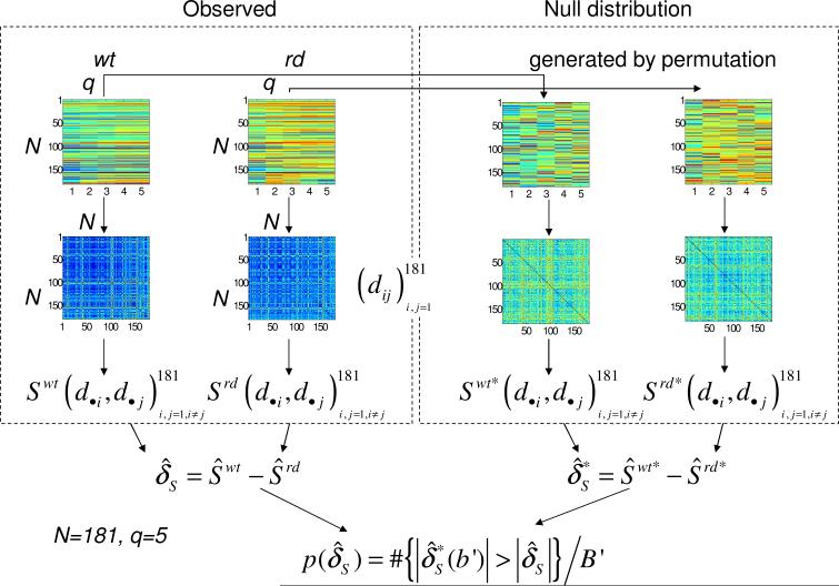
Correlation change (δ_M, δ_C and δ_MI) was evaluated based on the Euclidean distances of expression profiles between wt and rd mice. We proceeded as follows. Average expression values of the duplicates were calculated for wt and rd mice, respectively. Next, distance matrices, $d_{ij}^{wt}$ and $d_{ij}^{rd}$, were generated for the wt and rd mouse, respectively, with the (i, j) entry denoting the Euclidean distance between the i-th and the j-th genes using the data from the time course (Fig. 5). For each pair of the genes (i, j) we evaluated M, C, and MI between the i-th and j-th columns of the distance matrix, resulting in a total of 16,290 pair-wise correlations pairs, one for wt and one for rd. The correlation is measuring the relationship between how gene i interacts with all the other genes vs. how gene j interacts with all the other genes. Finally, correlation change between wt and rd mice, δ_S (S = M, C, MI), was evaluated using (4). The values of association change based on Spearman's rank correlation coefficient and Pearson's correlation coefficient are almost identical. Also, these two methods had very similar performance on 12 simulated cases. Therefore, δ_Spearman is not included in the results for the expression data.

Figure 5.

Data setup and permutation test to test association change for microarray expression data. Association change δ_S (S = M, C, and MI) between distances (d_ij) of expression profiles between the control (wt) and treatment (rd) group. In our study, N = 181, and q = 5.

Nonlinear correlation in expression data

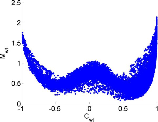
Plotting Pearson's correlation C against M for each of the pair-wise correlations, results in a W shaped relationship (Fig. 6). That is, when Pearson correlation C is low, maximal local correlation M could be high, the portion reflected by the middle of the W. This phenomenon, however, is not vice versa. In addition, two sides of the W indicate that when C is high, the value of M is also high as well. In other words, this W shaped relationship indicates that maximum local correlation can capture local correlation observed in the biological dataset, which can not be detected using Pearson's correlation C. Figure 1 shows an example of correlation between two genes that can only be detected by nonlinear correlation measures (M = 0.93, p = 0.007; MI = 1.15, p = 0.01) but not by linear correlation (C = –0.08, p = 0.88; S = –0.21, p = 0.67). This is due to the fact that signals are partially positively and partially negatively correlated (e.g., Fig. 1). The agreement between M and MI is high across all pairs of genes (C = 0.81, p ≈ 0).

Figure 6.

The “W” shape relationship between Pearson correlation (C) and maximum local correlation (M). This indicates that M captures additional information. Some local correlation can only be detected by M, but not by C.

4.1 Identification of Critical Genes by Correlation Change

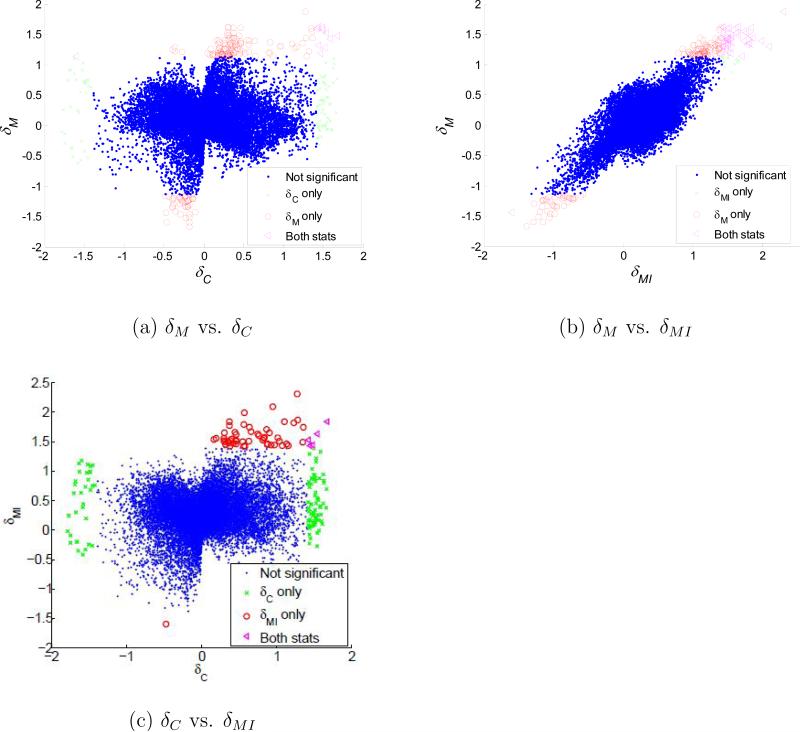
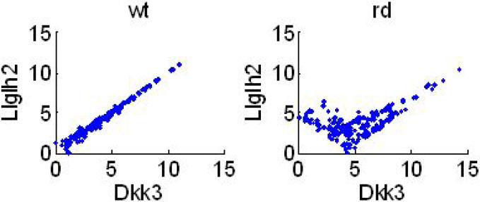
Association changes (δ_M, δ_C and δ_MI) between wt and rd animals were estimated for each pair of genes. Their p-values were estimated using (B.1) in Appendix B and corresponding q-values were estimated (Storey and Tibshirani, 2003). A total of 75 genes with at least one significant association change was detected using δ_C when controlling FDR at 0.05. In a similar manner, 137 genes with at least one significant association change were detected using δ_M, and 67 genes were detected using δ_MI when controlling FDR for each statistic at 0.05. The ranked importance of the candidate genes involved in rod degeneration is based on the frequency of association change with statistical significance. Some association changes are detected by both δ_M and δ_C statistics, but not all (Fig. 7a). The linear correlation between δ_M and δ_C is weak but significant (C = 0.03, p ≈ 4.4 · 10^–5). Out of the selected candidate genes with significant association changes between control and disease states using δ_M and δ_C, 62 of the probes were selected by both statistics, 75 of them could only be detected using δ_M whereas 13 of them were only detected using δ_C. The overall agreement between δ_M and δ_MI, in contrast, is high (C = 0.74, p ≈ 0), especially for large values (Fig. 7b). This is consistent with the earlier observation that M and MI have relatively high concordance. When controlling FDR at 0.05 for each statistic, δ_M can detect more association change (170 changes) between rd and wt mouse with statistical significance than those detected by δ_MI (58 changes; Fig. 7b). Fig. 8 shows an example of an association change between genes, and this association change can only be detected using δ_M (δ_M = 1.22, p ≈ 0), but not by δ_C (δ_C = 0.47, p = 0.32) nor by δ_MI (δ_MI = 1.32, p = 0.001). In the wt mouse, the correlation between the two genes is linear, but the association becomes a nonlinear (partially positively and partially negatively) correlation in the rd mouse.

Figure 7.

Scatter plot between different association changes measured between wt and rd mouse. (a) δ_M and δ_C can identify different association changes; (b) δ_M and δ_MI have high concordance, and identify more significant correlation changes than δ_C. (c) The relationship between δ_Cn and δ_MI is similar to that between δ_C and δ_M in (a).

Figure 8.

An example of the local association change between two states (rd and wt). This association change can only be detected with statistical significance using δ_M but not δ_C or δ_MI.

4.2 Validation of the Selected Candidate Genes

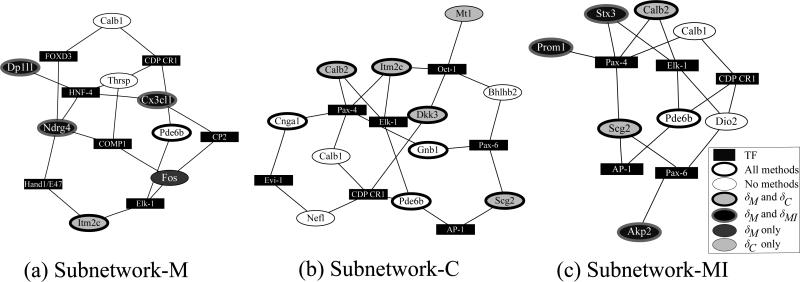
Given the current status of the literature on photoreceptor degeneration, much of the physiology still remains unclear. Knowing this, the results for δ statistics were evaluated through the following means. First, based on the fact that photoreceptor cell death in the rd mouse retina is caused by a mutation in Pde6b, leading to the complete loss of Pde6b mRNA expression, it is expected that a successful method will identify Pde6b as a high-ranked gene; i.e., Pde6b serves as a positive control. Indeed, Pde6b is ranked as the number 1 gene using either of the three statistics (Table 2). Second, the ultimate goal is to identify marker genes that are able to correctly recognize physiological processes (i.e., photoreceptor degeneration) and to identify key regulatory genes involved in this process. Thus, criteria for genes that accurately reflect the biological process might be (a) sharing similar expression profiles with genes involved in photoreceptor development, and (b) the involvement of their gene products in processes such as cellular stress response, cellular homeostasis, or others. These key regulatory genes might encode for transcription factors, growth factors or their receptors, anti-apoptotic genes, etc. To identify genes induced during the period of photoreceptor development, Pde6b was used as the bait gene to identify the 180 neighboring genes whose expression profiles cluster with Pde6b during development (http://cepko.med.harvard.edu/default.asp) (Black-shaw et al., 2001). Twenty-two of these neighboring genes were in the list of genes analyzed in this study. We then compared these genes against the candidates selected by each δ statistic. Among those, δ_C identified 9 of them, δ_MI identified 11, whereas δ_M identified 21 of the 22 possible genes, suggesting that δ_M was able to identify more photoreceptor-specific genes. The known biological roles of the top ranked genes for each method are summarized in Table 3. Interestingly, δ_M identified 3 transcription factors known to be involved in neuronal degeneration and cellular stress responses, whereas δ_C and δ_MI identified only 1 each, again suggesting that δ_M could identify more regulatory genes. To further evaluate the performance of the developed statistic, a gene regulatory network was constructed for the 181 analyzed genes using transcription factor binding sites to establish node connectivity (see Appendix D for details). Briefly, the top ranked genes generated by each of the statistics (Table 2) were used as “seed genes” to find a subnetwork of pairwise shortest paths in order to summarize the genes’ relationships. Each set of top ranked genes generated by each statistic (Table 2) was used to establish each of the subnetworks, subnetwork-M, subnetwork-MI, and subnetwork-C, depicted in Fig. 9. Let A_M, A_MI, and A_C denote the sets of “discovered genes”, discovered independently of their expression levels, in the three subnetworks. The underlying assumption is that the discovered genes in A_S (S = M, MI, C) may also play important roles as the “seed genes” since they are likely regulated by the same transcription factors. We asked whether these genes in A are also recognized by the δ statistics, and how do they compare to each other. Almost all of the genes in A_M, A_MI, and A_C are also identified as candidate genes by δ_M (Fig. 9), with a few exceptions, Thrsp, Nefl, and Mt1. Among those, Thrsp and Nefl were not identified by any of statistics. Thus, the resulting “discovered” genes are in high agreement with the listed genes selected by no matter which set of “seeds” we started with. This is not the case for δ_MI and δ_C. There is at least one or more genes that can not be identified by δ_MI and δ_C in each of the 3 subnetworks.

Table 2.

Top ranked candidate genes in rod degeneration for rd mouse

Rank	δ M		δ C		δ MI
	Gene	f	Gene	f	Gene	f
1	Pde6b	16	Pde6b	54	Pde6b	14
2	Dp1l1	15	Cnga1	22	Stx3	4
3	Fos	8	Pde6b	19	Prom1	4
4	Ndrg4	7	Gnb1	10	Akp2	4

f : observed frequency of association change with other genes between wt and rd mouse with statistical significance.

Table 3.

Known biological function of the top 25* candidate genes identified by δ_M, δ_C and δ_MI for six criteria (transcription factor, mutations in genes that are known to cause retinal degeneration, gene products involved in regulating apoptosis, gene products that are known photoreceptor structural genes or are involved in the photoreceptor signal transduction cascade, stress-induced genes and genes involved in calcium or ion binding as the genetic mutation in the rd mouse causes calcium overload in the photoreceptors.

Function	δ M	δ MI	δ C
Transcription factors:
	Csda, Fos, Gas6	Gas6	DKK3
Disease genes:
	Pde6b, Promt, Rho	Pde6a, Pde6b, Cnga1, Prom1	Pde6b, Gnat2 Cngal
Regulator of apoptosis:
	Aldh1a1, Tnfsf12	Tnfsf12	Aldhlal, Eefla2
photoreceptor structural genes:
	Pde6b (2), Cacnb2, Rho, Prom1	Gnbl, Pde6b, Roml, Cngal, Pde6a, Cacnb2, Gnbl	Pde6b (2), Cngal Gnbl, Gnat2
stress genes:
	Usp2, Pcp4, Clu, A2m	Clu	Clu, Mtl, Mt2
Ca2+ or ion binding:
	Pcp4, Slc4a7, Calb2, Vsnll, B2m	Vsnll, Sparcll	Spock2, Pcp4, Vsnll Calb2

Due to tied ranks, 26 genes are used as cut off for δ_M, 25 for δ_MI, and 27 for δ_C.

Figure 9.

Three subnetworks, subnetwork-M, subnetwork-C, and subnetwork-MI generated using transcription factor binding information. These subnetworks were generated automatically using the top-ranked genes selected by (a)δ_M, (b)δ_C, and (c)δ_MI, respectively, as “seeds”. Independent of correlation of expression, transcription factor (TF) binding information was then used to “discover” other important genes connected to the “seeds”. The legend of the genes indicates whether these seed or discovered genes are also identified by statistics as important candidates. “All” means all three methods, and “none” means none of the statistics.

Is the subnetwork-M (Fig. 9) plausible for further experimental assessment? c-Fos, a transcription factor, is known to be induced in the rd rods prior to degeneration (Rich et al., 1997), but was not essential for rod degeneration in this particular mouse model (Hafezi et al., 1997). Itm2C, a relatively unknown gene, interacts with the beta-site APP-cleaving enzyme 1, a protease important in the pathogenesis of Alzheimer's disease (Wickham et al., 2005). It is plausible that over-expression of this protein might be involved in rod degeneration. Dp1l1 is a protein presumably associated with membrane trafficking (Sato et al., 2005). Loss of Dp1l1 expression may be a reflection of cell loss, or alternatively suggest that disrupted cellular homeostasis in the rd rods leads to a secondary defect in membrane trafficking. Follow-up experiments are required to test the potential roles of these genes in the regulation of rod degeneration.

4.3 Discussion

In Section 3, we demonstrated that our proposed metrics, local correlation (ℓ; Fig. 4) and maximum local correlation M (Table 1), can quantify generic nonlinear associations in all simulated cases that have been designed with some degree of association. This is in contrast to Pearson's or Spearman's correlations, which were not able to detect significant association when the data was not linear in nature.

In Section 4, we applied the proposed method to identify genes related to rod degeneration. The data were microarray expression data of healthy and mutant animals. All three δ statistics, δ_C, δ_M, and δ_MI, correctly identified Pde6b, the defective gene in the rd mouse, as the most central gene in the degeneration process, validating our method. Furthermore, δ_M selected more genes involved in photoreceptor development (the presumed inverse of photoreceptor degeneration), and more plausible key regulatory genes involved in the process of cell death when compared to δ_C, which selected genes whose expression appears changed as a response to death (Table 3). The discordant results between nonlinear and linear methods (Fig. 7a) as well as the concordant findings between δ_M and δ_MI (Fig. 7b) further emphasize the importance of the development of statistics to measure nonlinear association instead of global linear patterns. In addition, δ_M has higher statistical power, and can detect more local correlation change than δ_MI when controlling FDR at the same level (Fig. 7b). Our method is not distributional based, and is instead an omnibus approach for detecting nonlinear correlations.

The challenges of nonlinearity and small sample size for the massive amount of data generated by modern high-throughput methods set the stage for the study described here. We have extended the use of correlation integrals to detect nonlinear correlation between any two variables reporting transient association. The proposed method is shown to have higher statistical power when compared with the reference use of mutual information and Pearson's correlation. Being distribution-free makes this tool applicable to a wide variety of problems. Although we only applied this approach to expression data in this study, the method can be applied to many other data, such as those generated by proteomics and metabolomics. In conclusion, the development of novel correlation methods that cope with the characteristic transient nonlinearity of biological dependencies, as assessed by the pairwise comparison study reported here, holds great promise.

The results of our study suggest a number of other avenues for future research. Our current work only focused on bivariate correlation. A natural extension would be the development of multivariate local correlations. Another extension would be to identify local group membership using the significant local correlation $\left(\ell \right)$ at particular scales of interest. Improvement of computational e ciency could also be a topic itself in the future since the computational complexity is O(N²) as it stands currently. More details on the computational complexity could be found in Appendix E. The relationship between linear and nonlinear association changes (Fig. 7) indicates that using both correlations yield more information. This also leaves open the question of the relationship between these statistics or the development of a new metric.

References

- Blackshaw S, Fraioli R, Furukawa T, Cepko C. Comprehensive analysis of photoreceptor gene expression and the identification of candidate retinal disease genes. Cell. 2001;107:579–589. doi: 10.1016/s0092-8674(01)00574-8. [DOI] [PubMed] [Google Scholar]
- Daub C, Steuer R, Selbig J, Kloska S. Estimating mutual information using B-spline functions - an improved similarity measure for analysing gene expression data. BMC Bioinformatics. 2004;5:118. doi: 10.1186/1471-2105-5-118. [DOI] [PMC free article] [PubMed] [Google Scholar]
- Efron B, Tibshirani RJ. an introduction to the bootstrap. Chapman & Hall/CRC; Boca Raton, FL: 1993. permutation tests., vol. 57 of Momographs on statistics and applied probability.
- Grassberger P, Procaccia I. Characterization of Strange Attractors. Physical Review Letters. 1983;50:346–349. [Google Scholar]
- Hafezi F, Abegg M, Grimm C, Wenzel A, Munz K, Sturmer J, Farber D, Reme C. Retinal degeneration in the rd mouse in the absence of c-fos. Invest Ophthalmol Vis Sci. 1997;39:2239–44. [PubMed] [Google Scholar]
- Jonnalagadda S, Srinivasan R. ISMB. iSMB; Glasgow, Scotland: 2004. An Information Theory Approach for Validating Clusters in Microarray Data. 2004. [Google Scholar]
- Kasturi J, Acharya R. Clustering of diverse genomic data using information fusion. Bioinformatics. 2005;21:423–429. doi: 10.1093/bioinformatics/bti186., clustering of diverse genomic data using information fusion.
- Kitano H. Computational systems biology. Nature. 2002a;420:206–210. doi: 10.1038/nature01254. [DOI] [PubMed] [Google Scholar]
- Kitano H. Systems Biology: A Brief Overview. Science. 2002b;295:1662–1664. doi: 10.1126/science.1069492. [DOI] [PubMed] [Google Scholar]
- Marshall E. Getting the noise out of gene arrays. Science. 2004;306:630–1. doi: 10.1126/science.306.5696.630. [DOI] [PubMed] [Google Scholar]
- Quackenbush J. Computational analysis of microarray data. Nat Rev Genet. 2001;2:418–27. doi: 10.1038/35076576. [DOI] [PubMed] [Google Scholar]
- Rich KA, Zhan Y, Blanks JC. Aberrant expression of c-Fos accompanies photoreceptor cell death in the rd mouse. Journal of Neurobiology. 1997;32:593–612. doi: 10.1002/(sici)1097-4695(19970605)32:6<593::aid-neu5>3.0.co;2-v. [DOI] [PubMed] [Google Scholar]
- Rohrer B, Pinto FR, Hulse KE, Lohr HR, Zhang L, Almeida JS. Multidestructive Pathways Triggered in Photoreceptor Cell Death of the RD Mouse as Determined through Gene Expression Profiling. J. Biol. Chem. 2004;279:41903–41910. doi: 10.1074/jbc.M405085200. [DOI] [PubMed] [Google Scholar]
- Sato H, Tomita H, Nakazawa T, Wakana S, Tamai M. Deleted in Polyposis 1-like 1 Gene (Dp1l1): A Novel Gene Richly Expressed in Retinal Ganglion Cells. Invest. Ophthalmol. Vis. Sci. 2005;46:791–796. doi: 10.1167/iovs.04-0867. [DOI] [PubMed] [Google Scholar]
- Steuer R, Kurths J, Daub CO, Weise J, Selbig J. The mutual information: Detecting and evaluating dependencies between variables. Bioinformatics. 2002;18:S231–240. doi: 10.1093/bioinformatics/18.suppl_2.s231. [DOI] [PubMed] [Google Scholar]
- Storey JD, Tibshirani R. Statistical significance for genomewide studies. PNAS. 2003;100:9440–9445. doi: 10.1073/pnas.1530509100. [DOI] [PMC free article] [PubMed] [Google Scholar]
- Vilela M, Borges CCH, Vinga S, Vasconcelos ATR, Santos H, Voit EO, Almeida JS. Automated smoother for the numerical decoupling of dynamics models. BMC Bioinformatics. 2007;8:305. doi: 10.1186/1471-2105-8-305., fully automated perfect smoother for numerical decoupling of multivariate, dynamic, S-System models.
- Wickham L, Benjannet S, Marcinkiewicz E, Chretien M, Seidah NG. Beta-Amyloid protein converting enzyme 1 and brain-specific type II membrane protein BRI3: binding partners processed by furin. Journal of Neurochemistry. 2005;92:93–102. doi: 10.1111/j.1471-4159.2004.02840.x. [DOI] [PubMed] [Google Scholar]