Simple, Inexpensive Attainment and Measurement of Very High Cooling and Warming Rates

Abstract

We have developed a simple, inexpensive system (< $300 US) for measuring cooling and warming rates of small (~ 0.1 μl) aqueous samples at rates as high as 10⁵ °C/min. The measurement system itself, can track rates approaching one million °C/min. For temperature sensing, a Type T thermocouple with 50 μm wire was used. The thermocouple output voltage was read with an inexpensive USB based digital oscilloscope interfaced to a laptop computer, and the raw data were processed with MS Excel.

Currently our group is investigating the effects and interactions of very high cooling and warming rates in cryobiology [5,8]. For this work, we have developed a simple, inexpensive (<300 $US) temperature measurement system [3]. The design goal was to measure the temperature of a 0.1 μl aqueous sample at rates up to 1 million °C/min using a temperature sensing element which would minimally perturb the system thermally. To achieve this, a simple, fine gauge thermocouple (TC) proved suitable.

Choice of Thermocouple

We chose a Type T thermocouple (TC) from those available in the Omega Engineering ® catalog under “Unsheathed Fine Gage Microtemp Thermocouples” [6]. Type T, E, and K are all suitable for low temperature measurements. Type E is desirable because it has a 50% higher sensitivity (μV/°C) than either Type T or K. Type E and K are both available in 13 μm wire size while the smallest gage Type T is 25 μm diameter. Ultimately we choose Type T (copper – constantan) as it is the best characterized and most common type. However, in retrospect, the higher sensitivity of Type E would have been useful given the noise levels in our electronics.

There are trade offs to be made in the TC wire size chosen. Smaller sizes perturb the cryo sample less. Also, smaller sizes yield faster response times; but they are more difficult to handle. Omega posts a table of response times for their unsheathed fine gage TC’s [7]. Specifically, they list the time constant, τ, of a 25 μm wire diameter TC as 0.002 seconds in making a step change from 200 °F water to 100 °F water (ΔT = 56 °C). Thus the TC reaches 63% of its final temperature after 0.002 seconds. Omega assumes a response curve of the form:

$$T=T0+\Delta T(1-e^{-t∕\tau }).$$

From this, we can estimate the highest cooling or warming rate to which such a TC can respond. In three time constants, a TC will reach 95% of the final temperature. Thus we estimate the maximum response rate, R, for a 25 μm wire TC as:

$$R=\Delta T∕\Delta t=56°\mathrm{C}∕(3\ast 0.002\sec )=5.6\times {10}^5°\mathrm{C}∕\min .$$

These data from Omega are for a Type J Iron-Constantan thermocouple. Here, we are considering a Type T Copper-Constantan TC.

When considering TC response times, both the heat capacity of the TC and the thermal resistance (or conductance) between the TC and the surrounding sample need to be considered. By thermal resistance, we are referring to the fact that it takes time for heat to flow through the bulk metal of the TC to the TC - sample interface, across the interface, and into the sample in which the TC is embedded. The experimental data from Omega reflects the influence of both. Here we assume that the thermal resistances of the Type J and T thermocouples, imbedded in identical samples, are the same for identically sized wires because they are made of similar materials. The other factor to consider is the heat capacity of the TC’s. For identically sized wires, this is proportional to Cp*ρ (specific heat capacity x density). For iron, Cp = 0.45 J/(gK) and ρ = 7.87 g/cm³; and for copper, Cp = 0.39 J/(gK) and ρ = 8.94 g/cm³. The Cp*ρ product for iron and copper differ by less than 2%. Thus the heat capacities of iron and copper wires are nearly identical and the thermal response time data from Omega for Type J should apply equally well to Type T thermocouples where, as noted above, we assume similar thermal resistance characteristics between the TC and sample. We expect these Type J response data to be a good approximation for all metal thermocouples.

Plotting all the response data from Omega as a function of TC wire area yields a relatively linear relationship as expected (the response time is proportional to the mass per unit length of the wire), Figure 1. We note, parenthetically, that the linear response in Fig 1 suggests that it is the thermal mass of the TC and not the thermal resistance, discussed above, which primarily determines the response speed of these metal TC’s. From Fig 1 we estimate the maximum rates attainable with 13, 25, and 50 μm diameter wire TC’s to be 2.2 × 10⁶, 5.6 × 10⁵, and 1.6 × 10⁵ °C/min, respectively.

Figure 1.

Response time constants for bare Type J thermocouples of varying wire size exposed to a 200 °F to 100 °F water step gradient. In one time constant the TC reaches (1 – 1/e) ≈ 63 % of its final value. Type T thermocouples are expected to have a similar response; see text. Data from Omega Engineering ® [7].

Although we were able, with some difficulty, to make some TC assemblies with 25 μm diameter wire, we eventually decided on the larger, 50 μm diameter wire, as more robust, and yet fast enough in response. In our subsequent tests on bare 50 μm Type T thermocouples, moved rapidly from LN₂ to room temperature water, we achieved warming rates of 3 × 10⁵ to 5 × 10⁵ °C/min, roughly consistent with a maximum rate of 1.6 × 10⁵ °C/min estimated on the basis of the published Omega data using a 3 τ response time. Thus Omega’s and our data indicate the 50 μm TC’s can track cooling/warming rates in excess of 100,000 °C/min.

Thermocouple Assembly on Cryotop®

As mentioned previously, we also require that our TC minimally perturb the thermal behavior of the cryo sample being cooled or warmed. In particular, we require that the heat capacity of the TC be small compared to the sample in which it is embedded. Figure 2 shows the TC junction and sample on a Cryotop ®. The Cryotop is a 20 × 0.4 × 0.1 mm flat polypropylene stick with handle and is frequently used as the carrier for small samples and high cooling and/or warming rates [2,4]. The fine TC wires were led to the end of the Cryotop handle where they were mated to standard gauge TC wire using an Omega SMPW-CC-T-M male plug. The strain relief of the plug nicely holds the Cryotop handle. Red nail polish was used to fix the fine TC wires to the polypropylene stick. Assembly was done under a stereo microscope at 15 X. The nail polish held up well under repeated LN₂ freeze-thaw cycles.

Figure 2.

0.1 μL aqueous sample (A) on a Cryotop ® tip (B) with a 50 μm wire lead Omega Cu-Constantan thermocouple (C) embedded in the sample. Red nail polish (D) is used to hold the TC in place.

For high cooling and warming rates we assume that only the mass in the vicinity of the sample comes into play as there is too little time for significant amounts of heat to flow to or from regions remote from the sample. Based on the physical size of the 0.1 μl sample (Fig 2), we take the thermally involved or relevant region to be the aqueous sample, a 1 mm length of polypropylene stick, and 1 mm × 2 of TC wire. Table 1 shows the thermal properties of this ‘involved’ region. As desired, the TC only represents a small, 5 %, contribution to the thermal mass of the system. The sample is the largest contributor, 71 %, and is thus the limiting factor in the thermal response of the system.

Table 1.

Sample/Assembly Thermal Properties

Substance	Mass	Cp	Heat Capacity	Thermal Mass4
-	(g)	(J/g/K)	(J/K)	(% Total)
Ice 1	10 × 10−5	2.1	2.1 × 10−4	71 %
Polyproylene 2	3.7 × 10−5	1.9	0.70 × 10−4	24 %
Wire 3	3.5 × 10−5	0.39	0.14 × 10−4	5 %

¹0.1 μL of water.

²1 × 0.4 × 0.1 mm of polypropylene; density assumed to be 0.92 g/cm³.

³1 mm Cu and 1 mm Constantan wire length, diameter 50 μm; density assumed to be 8.9 g/cm³.

⁴These are computed by summing the heat capacities in column four and dividing this result into the individual heat capacities.

Measurement System

Our second requirement was to develop a simple, inexpensive measurement system capable of following the TC output voltage at rates up to 10⁶ °C/min. For a sample chilled to LN₂ temperatures, the cryobiologically relevant phenomena will occur between 0 °C and −200 °C. Since Rate = ΔT/Δt; in this example Δt = (200 °C)/(10⁶ °C/min) = 12 msec. Thus, for a simple thermal ramp, such as a plunge from room temperature to LN₂, or the converse, 1000 temperature measurements per second is adequate as this would yield ~12 temperature points during the cooling or warming ramp. This is 10 to 1000 times the speed of typical TC readout systems. To achieve this higher rate, we chose to use a digital storage oscilloscope. These easily achieve sampling rates 100’s of times our requirement.

The essential cost-saving step was to use a USB instrument which plugs into the USB port of an ordinary laptop computer. The laptop provides the power, brains, and display for the instrument. ‘Inexpensive’ digital USB scopes are available in the price range from $100 to $2,000 US. We decided on the very simple, intuitive to use, StingRay DS1M12 from EasySync Ltd for $220 US [1]. It is the size of a small paperback book. This unit offers 12 bit resolution, a maximum sensitivity of ± 10 mV full scale (perfect for the 6 ½ mV swings of Type T thermocouples between room and LN₂ temperatures) and it can easily record and store 10 to 20 seconds of data. With our thermocouple setup, the system noise was about ± 0.2 mV PTP which translates to a temperature noise of ≈ ± 2.5 °C RMS. For temperature excursions of 100 °C this yields an accuracy in the cooling/warming rate of a few percent, more than adequate for our needs. This error could be nearly halved by using a higher sensitivity Type E thermocouple. In conventional TC measurement systems of higher thermal accuracy, it is the need to average the noise over some small interval of time which leads to the low readout rates found in such systems.

Our system makes four sacrifices in the interest of simplicity and low cost. First, as just noted, noise limits the temperature accuracy to a few degrees. Second, the output of the USB scope is voltage, not temperature. Voltage is easily converted to temperature using a spreadsheet such as MS Excel and Emf to temperature conversion routines based on standard TC Tables. We found, for spreadsheet calculations, that a 4^th order polynomial gives better than 1 °C accuracy for a Type T thermocouple between +40 to −200 °C. Third, we do not use a TC reference junction in the system. Instead the temperature of the room/equipment is measured and the appropriate TC table Emf (~ 0.9 mV) is subtracted from the TC readings. Fourth, the inexpensive DC amplifier in our scope (as well as possible small room temperature wire junction effects) produced a small output offset voltage of 50 to 100 μV which we measured at the beginning of each run and corrected for in our Excel spreadsheet. By output offset voltage, we mean that with the instrument at room temperature and the TC at room temperature, the output differed by as much as 50 to 100 μV from the expected value of zero.

Typical Performance

A representative run of the system is shown in Figure 3 (top panel) in which a small aqueous sample (EAFS 10/10 vitrification solution consisting of ethylene glycol, acetamide, Ficoll, sucrose and salts in water, see [8]) is abruptly transferred from room temperature air to LN₂, held 4 sec, and rapidly returned to room temperature water. The rate of temperature change in the region of interest is easily determined to good accuracy with a visually fit slope line despite the system noise (bottom panel). In practice this system has proven robust and easy to use; although some skill is required in assembling the Cryotop and thermocouple under the stereo microscope.

Figure 3.

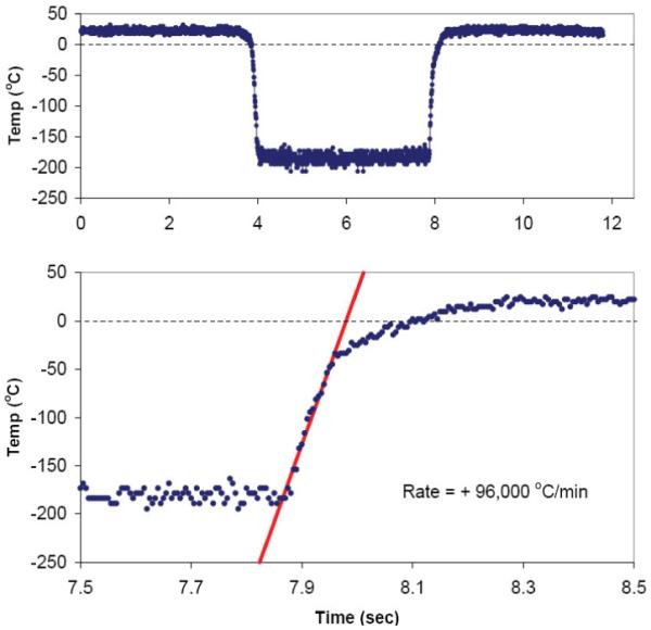
(Top panel) Thermal cycle of a 0.1 μL aqueous sample (EAFS 10/10 vitrificatrion solution [8]) on a Cryotop ® instrumented with a 50 μm Cu-Constantan thermocouple and rapidly moved from room temperature air to LN₂, held 4 sec, and rapidly immersed in a room-temperature water bath. (Bottom panel) Details of events during warming between ~7.8 sec and 8.0 sec when the sample was moved from LN₂ to room temperature water The upward sloping straight line was visually fit to the data and yields the warming rate of 96,000 °C/min. The temperature sampling rate is 200 readings per sec.

References

- [1].EasySync Ltd . Hillsboro, Oregon, USA: http://www.easysync-ltd.com/ [Google Scholar]
- [2].Kitazato Biopharma . Japan: http://www.kitazato-biopharma.com/cryotop/method.html. [Google Scholar]
- [3].Kleinhans FW, Seki S, Mazur P. Abstract presented at Cryo-2009: Simple, inexpensive measurement of very rapid cooling and warming rates. Cryobiology. 2009;59:381. doi: 10.1016/j.cryobiol.2010.06.011. [DOI] [PMC free article] [PubMed] [Google Scholar]
- [4].Kuwayama M. Highly efficient vitrification method for cryopreservation of human oocytes. Reproductive BioMedicine Online. 2005;11:300–308. doi: 10.1016/s1472-6483(10)60837-1. [DOI] [PubMed] [Google Scholar]
- [5].Mazur P, Seki S, Kleinhans FW. Abstract presented at Cryo-2009: Survival of mouse oocytes suspended in EAFS 10/10 vitrification solution after being cooled to −196 °C on Cryotops at rates ranging from 95 °C/min to 70,000 °C/min and warmed at 610 °C/min to 118,000 °C/min. Cryobiology. 2009;59:396. [Google Scholar]
- [6].Omega Engineering Inc. Stamford, Connecticut, USA The 50 μm wire Type T thermocouple is part # COCO-002. I.e. Copper-Constantan 0.002” wire thermocouple. http://www.omega.com/
- [7].Omega Engineering Inc. Stamford, Connecticut, USA These response data appear on the web order page for “Unsheathed Fine Gage Microtemp Thermocouples, J, K, T, E, R &S”. specifically: http://www.omega.com/ppt/pptsc.asp?ref=IRCO_CHAL_P13R_P10R&Nav=tema02.
- [8].Seki S, Mazur P. The dominance of warming rate over cooling rate in the survival of mouse oocytes subjected to a vitrification procedure. Cryobiology. 2009;59:75–82. doi: 10.1016/j.cryobiol.2009.04.012. [DOI] [PMC free article] [PubMed] [Google Scholar]