The Lexical Restructuring Hypothesis and Graph Theoretic Analyses of Networks Based on Random Lexicons

Abstract

Purpose

The mental lexicon of words used for spoken word recognition has been modeled as a complex network or graph. Do the characteristics of that graph reflect processes involved in its growth (M. S. Vitevitch, 2008) or simply the phonetic overlap between similar-sounding words?

Method

Three pseudolexicons were generated by randomly selecting phonological segments from a fixed set. Each lexicon was then modeled as a graph, linking words differing by one segment. The properties of those graphs were compared with those of a graph based on real English words.

Results

The properties of the graphs built from the pseudolexicons matched the properties of the graph based on English words. Each graph consisted of a single large island and a number of smaller islands and hermits. The degree distribution of each graph was better fit by an exponential than by a power function. Each graph showed short path lengths, large clustering coefficients, and positive assortative mixing.

Conclusion

The results suggest that there is no need to appeal to processes of growth or language acquisition to explain the formal properties of the network structure of the mental lexicon. These properties emerged because the network was built based on the phonetic overlap of words.

Understanding how children add words to their mental lexicon, how they represent the sound patterns of those words in their lexicon for purposes of recognizing spoken words, and how those representations possibly change over time are all critical to understanding the more general problem of language acquisition. The lexical restructuring hypothesis (e.g., Metsala 1997a, 1997b; Walley, 1993, 2005) has been particularly influential in this area. According to this hypothesis, a word’s representation in the mental lexicon changes over time from a relatively holistic representation to a much more detailed and segmental representation. Holistic representations suffice when the child knows only a few words. As vocabulary grows, however, and more words are added to the lexicon that are phonologically similar to words already part of the lexicon, their lexical representations evolve to ones with the more detailed, segmental information needed to discriminate similar-sounding words. Lexical restructuring does not occur all at once for the entire lexicon. Rather, it occurs for a particular word as that word acquires phonological neighbors and becomes part of a larger set of similar-sounding words.

Various behavioral data have been adduced in favor of the lexical restructuring hypothesis. Metsala (1997a), for instance, compared the performance of children from three different age groups and adults using a word gating paradigm (Grosjean, 1980). She used decreases in the gate duration required to recognize a word as an indicator of segmental representation for that word. High-frequency words with many neighbors were predicted to more likely require early restructuring—and thus show signs of segmental representation—than less frequently encountered words or words from less densely populated neighborhoods. In agreement with that prediction, Metsala found no significant differences in the gate duration required for spoken word recognition between the various age groups for high-frequency words from dense neighborhoods. Presumably, these words were represented segmentally by all age groups. In contrast, gate durations were longer for children than adults (and for 7-year-olds than for 11-year-olds) for high-frequency words from sparse neighborhoods. Because of the sparseness of the neighborhoods, there is less pressure on children to represent the fine phonetic detail of these words. They can rely on more holistic representations. However, partial input cannot match a holistic representation and, hence, children require more input (i.e., greater signal durations) to recognize these words. Adults, in contrast, can use their lexical knowledge of segments to recognize even words from sparse neighborhoods based on incomplete phonetic input (Metsala, 1997a). Also in line with the predictions of the lexical restructuring hypothesis, Metsala found that younger children required longer gate durations than did older children and adults to recognize low-frequency words from both sparse and dense neighborhoods.

Charles-Luce and Luce (1990, 1995) reported that words in younger children’s lexicons generally formed less dense neighborhoods than words in older children’s lexicons. Likewise, words in older children’s lexicons formed less dense neighborhoods than words in the lexicons of adults. These findings indicate that the need for more detailed segmental representations of spoken words increases with age.

In a more recent study, Storkel (2002) examined children’s judgments of the sound similarity of different word pairs. She found that similarity judgments for words overlapping in the onset and nucleus and for words overlapping in the nucleus and coda were affected by phoneme similarity (i.e., segmental representations) for words from dense neighborhoods. For words from sparse neighborhoods, similarity judgments for words with overlap in the onset and nucleus were driven by phoneme similarity but were driven by manner similarity (a more holistic representation) for words from sparse neighborhoods with overlap in the nucleus plus coda. Based on these results, Storkel argued for a weak lexical restructuring hypothesis. According to her account, segmental representations are available even to young children. What changes with age (and task demands) is not the availability of segmental representations but which aspects of the representation the child focuses his/her attention on in order to complete the task.

Not all data, however, unambiguously favor the lexical restructuring hypothesis. Dollaghan (1994) found that the vast majority of children’s words have at least one phonological neighbor. Consequently, the representation in the mental lexicon must contain some detailed phonetic information. Coady and Aslin (2003) showed that when neighborhood density is normalized by vocabulary size, density actually decreases with age. Lexical restructuring predicts that density should increase with age. Swingley and Aslin (2002; see also Swingley, 2003) showed that 14- and 15-month-old infants were sensitive to mispronunciations as small as a single phonetic feature, suggesting that the lexical representations of these children are quite precise and well-specified and contain a large amount of segmental detail. This effect held even for words that, according to an analysis of the child’s receptive vocabulary, had no lexical neighbors. Similarly, R. S. Newman (2008) has argued that infants’ mental representations of spoken words contain so much detail that it can actually hinder their ability to recognize spoken words.

Recently, Vitevitch (2008) introduced a novel and potentially quite powerful source of data that is relevant to the lexical restructuring hypothesis. He modeled the mental lexicon as a graph or complex network. He then analyzed various properties of that graph and asked what network growth or developmental process could produce a graph with those properties. Before reviewing his results in detail, we first provide some background on graph theory that is necessary for understanding his results and the new findings presented in this article. (See Harary, 1969, for a detailed text on graph theory. Higgins, 2007, provides a less formal account oriented toward the nonmathematician. See Barabási, 2002, for a very readable review of applications of graph theory to complex systems.)

Overview of Graph Theory

Over the last decade or so, a number of researchers from a diverse set of disciplines have used the tools of graph theory to model complex systems (see Albert & Barabási, 2002, and Barabási, 2002, for reviews). In a graph or network, entities are represented by nodes, and relations between two entities are represented by links or edges between those nodes. When modeling the World Wide Web, for example, each Web site can be represented as a node (Pastor-Satorras & Vespignani, 2004). A link between two such nodes represents the fact that one of those Web sites has a (Web) link to the other. Two nodes with a link (in the graph-theoretic sense, not the Web sense) between them are sometimes referred to as neighbors.

A typical finding of studies modeling complex systems using graph theory is that such systems tend to have a small-world, scale-free structure (Barabási & Albert, 1999; Watts & Strogatz, 1998). Small-world networks are characterized by two properties (Watts & Strogatz, 1998). First, they have a relatively small mean shortest path length. The shortest path length between two nodes is the minimum number of links that needs to be traversed to get from one of those nodes to the other. The mean shortest path length is the mean of that minimum across all possible pairs of nodes in the network. In a small-world network, the mean shortest path length is of about the same size as the path length in a random, Erdos-Rényi (Erdos & Rényi, 1960) graph. (In an Erdos-Rényi graph, the number of nodes in the graph is fixed, and links are placed between nodes randomly with some fixed probability.) Second, small-world networks have a mean clustering coefficient (CC) that is much larger than what would occur in a random, Erdos-Rényi graph. The CC of Node A is a measure of the probability that any two neighbors of Node A are also neighbors of one another, with a higher probability corresponding to a higher CC.¹

Scale-free networks are defined by the form of their degree distribution (Barabási & Albert, 1999). A node’s degree is simply the total number of links attached to the node. The degree distribution is the frequency distribution of the degree across all nodes in the graph. A scale-free network² is characterized by a degree distribution that for large degrees follows a power law, N(k) ~ k^−γ, where N(k) is the degree distribution, k is the degree (i.e., the number of edges going into or coming out of the node), and the exponent, γ, is typically between 2 and 4.

Knowing a network’s structure and internal organization can be important because it has implications for how that network evolved over time. For example, a network that grows over time (i.e., nodes are added over time) and in which new nodes link to existing nodes with a probability proportional to the degree of that existing node (a process known as preferential attachment) shows a degree distribution with a power law tail (Barabási & Albert, 1999). That is, such networks are scale free. In contrast, a network that grows over time but in which new nodes link to existing nodes with a fixed probability results in an exponential degree distribution for large degrees (Barabási & Albert, 1999; Gruenenfelder & Mueller, 2007). A network that does not grow over time but whose nodes attach to one another with a fixed probability (i.e., a random Erdos-Rényi graph) results in a Poisson degree distribution.

Applying Graph Theory to the Mental Lexicon

In his pioneering paper, Vitevitch (2008) used the tools of graph theory to model the mental lexicon for spoken word recognition. Each word in the Hoosier Mental Lexicon (HML; Nusbaum, Pisoni, & Davis, 1984), a corpus of approximately 20,000 American English words based on Webster’s Seventh Collegiate Dictionary (1967), was represented as a node in the graph or network. A link or edge was placed between two nodes if the words represented by those nodes could be changed into one another by the deletion, addition, or substitution of a single phoneme (Greenberg & Jenkins, 1964; Landauer & Streeter, 1973; Luce & Pisoni, 1998). Two nodes joined by a link are frequently referred to as neighbors.

The resulting graph created by Vitevitch (2008) displayed five major properties. First, it consisted of many hermits (more than 10,000—i.e., over 50%—of the words), a multitude of small islands, and a single large island consisting of 6,508 words. (A hermit is a node that has no neighbors—i.e., it has no links to other words in the network. An island is a set of nodes, each of which can reach any other node in the island by traversing some number of links but none of which can reach any node in the overall network that is not in the island.) Thus, the mental lexicon is neither homogenous nor uniform. Second, for the large island, Vitevitch found that the mean shortest path length was small and not much larger than what would be expected in an Erdos-Rényi random graph. Third, the mean CC for the nodes in that large island was much greater than the mean CC of a comparably sized Erdos-Rényi random network. These last two properties suggest that the mental lexicon for spoken word recognition has a small-world structure (Watts & Strogatz, 1998)—any node is easily reachable, in terms of the number of links traversed, from any other node. Fourth, despite a number of a priori reasons for hypothesizing a power law degree distribution (see Vitevitch, 2008, for an explanation of these reasons), the large island in the network showed an exponential degree distribution. Fifth, the large island also showed an extraordinarily high degree of positive assortative mixing (M. Newman, 2002; M. Newman & Park, 2003). In a graph with positive assortative mixing, a node with many neighbors tends to have neighbors that also have many neighbors. In a graph with negative assortative mixing, or dissortative mixing, nodes with many neighbors tend to have neighbors that themselves have few neighbors. The extent of assortative mixing can be measured by correlating a node’s degree with the degree of all its neighbors. A positive correlation indicates positive assortative mixing; a negative correlation indicates dissortative mixing. For the large island, Vitevitch found this correlation to be +.62, indicating strong assortative mixing. That is, the neighbors of nodes with many (few) neighbors tend themselves to have many (few) neighbors. The rich not only get richer, as in Barabási and Albert’s (1999) preferential attachment model, but the rich also tend to associate with the rich.

Vitevitch (2008) argued that this pattern of results is consistent with a model that focuses on how the network grows over time. At a point in time, when a node (a word) is added to the network (the mental lexicon), it attaches to each of the existing words in the lexicon with some probability, p. Because p is less than 1, it is possible that the new node makes no connection with any existing node and remains a lexical hermit. In addition, two nodes previously unconnected with one another may at a later point in time form a connection with each other. Applied to the specific arena of language acquisition, Vitevitch suggested that such new connections could be formed via lexical restructuring (e.g., Metsala 1997a, 1997b; Walley, 1993, 2005).³

Callaway, Hopcroft, Kleinberg, Newman, and Strogatz (2001) have shown that a network that grows with the characteristics discussed by Vitevitch (2008) has a single large island and multiple hermits, an exponential degree distribution, and shows positive assortative mixing, in agreement with Vitevitch’s observations of the mental lexicon. Indeed, to the extent that the type of restructuring Vitevitch discusses (addition of links between previously unconnected nodes over time) were necessary to produce the network structure he observed, the lexical restructuring hypothesis would receive strong support. Even if lexical restructuring was shown to be sufficient but not necessary to produce the observed network properties, then, in the absence of a simpler alternative account, his results would still favor the lexical restructuring account of lexical development.

We are concerned, however, with attempts to explain the graph theoretic properties of the mental lexicon by appealing to principles of how that network grew over time. The mental lexicon certainly grows over time. Furthermore, in many areas (e.g., the World Wide Web, the structure of the Internet, the power grid—see Albert & Barabási, 2002, and Barabási & Albert, 1999, for a number of such examples), the current structure of a complex network can be explained by how the graph grew. Note, though, that in cases such as the Web and others reviewed by Albert and Barabási, there is no predefined endpoint structure to which the system had to evolve. The network could evolve to wherever its growth process took it. In the case of the human mental lexicon, however, there is a common lexicon of words in the language that each individual’s lexicon in a given linguistic community must approach. If there were no such common lexicon, communication would fail (and it would not make sense to use a corpus such as the one used by Vitevitch to model the mental lexicon). In other words, there is a pre-defined, final target lexicon that must be learned by each speaker-hearer of the language. Regardless of the development process, the process must converge to that common lexicon. One child could, on Day 1, learn one new word, on Day 2 learn two new words, on Day 3 learn four new words, and so on. Another child could first learn all words beginning with /i/, then all words beginning with /b/, and so on. A third child could begin by learning words that occur frequently in contexts important to the child and then proceed to learning less frequently occurring words. In the end, the same common lexicon would be learned by all three processes, and it would have the same formal graph theoretic properties regardless of the learning strategy used. (Clearly, two of the above developmental processes are implausible. They simply serve to make the point that when the final structure of a network is relatively fixed, the static graph theoretical properties of that structure may not help us understand how it developed.)

An Alternative Account of the Graph Theoretic Properties of the Mental Lexicon

Nevertheless, the new properties of the mental lexicon observed by Vitevitch (2008) do require an explanation. Furthermore, as pointed out by Vitevitch, the growth-plus-lexical restructuring process could occur over a relatively short time frame, corresponding to language acquisition, or over a much longer time frame, corresponding to the evolution of the common lexicon—that is, the addition of words to (and possible removal of words from) a linguistic community’s common lexicon over time. Because there is no pre-defined structure to which that common lexicon must evolve, the above argument does not apply to the case of language evolution. Growth-plus-lexical restructuring could explain how words are added to the language over time and thereby account for the occurrence of the five properties under consideration. Before accepting that explanation, however, simpler explanations need to be ruled out. One possible simpler explanation is that those properties are a consequence of how the original graph was constructed. Words were linked based on their phonetic overlap. Perhaps, when wholes (words, in the present case) are made up of a random sequence of parts (phonological segments, in the present case), and those wholes are then linked into a graph based on the overlap of their parts, the same five graph theoretic properties observed by Vitevitch would emerge even without any appeal to growth or restructuring processes. We refer to this hypothesis as the part-overlap hypothesis. One of our goals in this article was to assess this explanation for the results reported by Vitevitch (2008).

Some simple analytical analyses suggest that at least one of Vitevitch’s results would be expected in such a random lexicon—that is, a lexicon in which words are formed by simply randomly sequencing phonological segments. Consider a word’s clustering coefficient (CC). Word A’s raw CC, referred to here as CCraw, is simply the number of neighbor pairs formed by Word A’s neighbors divided by the total number of possible neighbor pairs that theoretically could be formed by Word A’s neighbors:

$$\text{CCraw}=\text{Na}/\text{Np},$$

where Na is the actual number of neighbor pairs and Np is the possible number of neighbor pairs. Consider a Word A with three neighbors: Words 1, 2, and 3. Note that among Word A’s neighbors, there are three possible neighbor pairs: Words 1 and 2, Words 1 and 3, and Words 2 and 3. Suppose that, in fact, Words 2 and 3 are neighbors but 1 and 2 are not, and 1 and 3 are not. Word A’s CCraw is then 1/3. If Words 2 and 3 are neighbors and 1 and 2 are also neighbors, but 1 and 3 are not neighbors, then the CCraw is 2/3.

Now consider a three-phoneme word, such as /sIt/ and all its three phoneme neighbors, such as /lIt/, /sIn/, /rIt/, and so on. Choose any two of those neighbors at random. By definition, the first of those neighbors differs from /sIt/ in exactly one phoneme position. Likewise, the second neighbor differs from /sIt/ in one phoneme position. Because both neighbors have three phonemes, the odds that neighbors 1 and 2 differ from /sIt/ in the same phoneme position, and hence are themselves neighbors, are 1 in 3. More generally, when only words with the same number of phonemes as the target word are considered, for three-phoneme words in a random lexicon, a CCraw of 1/3 would be expected. A CCraw value of 1/3 is a truly large CC. Likewise, for two phoneme words, the expected value of CCraw (when only two phoneme neighbors are considered) is 0.50, for four phoneme words it is 0.25, for five phoneme words it is 0.20, and so on.

The high values of CC reported by Vitevitch (2008) for words in the HML would thus be expected in a random lexicon—that is, a lexicon in which a word consists of a random sequence of segments. Such an analytical approach to the remaining four characteristics under discussion is less tractable. Consequently, we tested the part-overlap hypothesis by creating pseudolexicons consisting of “words” of randomly sequenced “segments.” Intuitively, we thought that we would need to introduce more and more phonotactic constraints into these lexicons before we saw all five properties observed by Vitevitch emerge. Consider, for example, the case of consonant clusters. We felt that these five core properties might not emerge until we had a sequence representing /fl/ and occurring with the same proportional frequency as /fl/ occurs in American English, another representing /tr/ and occurring with its same proportional frequency, and so on. Hence, we began our modeling work with relatively unconstrained lexicons with the plan of building more and more phontotactic constraints into them. As it turned out, however, such a plan was unnecessary because all five properties emerged in even relatively unconstrained pseudolexicons.

We report the results here for three such pseudolexicons. Each pseudolexicon used the same number of “consonant” segments and “vowel” segments as used in the phonetic transcriptions in the HML (Nusbaum et al., 1984). Words in the lexicons were generated by first determining the word length and then randomly sampling a segment (with replacement) for each segment position in the word. To keep the simulations manageable, we used word lengths of two through five segments, inclusive. In all the pseudolexicons, the same number of two-, three-, four-, and five-segment words were generated as are contained in the HML.

The lexicons differed from one another by the phonotactic constraints that were included—successive lexicons included successively more constraints. The Word Length Only (WLO) lexicon contained the same number of two-, three-, four-, and five-segment words as the HML. For example, the HML contains 3,120 words that are five segments in length. Hence, 3,120 five-segment words were randomly generated for the WLO lexicon. These words were constructed without regard to their consonant–vowel (CV) structure—/iIi/ and /bbb/ were both legitimate three-segment words within this lexicon. The CV Pattern (CVP) lexicon followed the word length constraint and, in addition, was constrained to generate the same number of words for each CV sequence as occurred in the HML. For instance, the HML contains 758 four-segment words with the sequence CCVC. Consequently, so did the CVP lexicon. Finally, the Word-Initial Consonant Cluster (WIC) lexicon followed both the word length constraint and the CV pattern constraint. In addition, for those words in which a WIC occurred, the initial consonant was constrained to be one of those segments that appears as the first segment in a word-initial English consonant cluster. The second segment was constrained to be a segment that appears in the second position of such a consonant cluster. No constraint was placed on which two consonants could co-occur in a cluster.⁴ For example, /b/ occurs as the initial segment in some English WICs. /p/ occurs as the second segment in other English WICs. Hence, in the WIC pseudolexicon, /bp/ would be an allowable word-initial cluster, even though the sequence /bp/ never occurs as a word-initial cluster in English. As this example suggests, even the WIC lexicon is still fairly unconstrained phonotactically relative to the observed patterns in English. We then compared the graph theoretic properties of these pseudolexicons to those of the subset of the HML consisting of all words two to five segments in length, as well as to the whole HML.

Method

Pseudolexicon Construction

Constructing and analyzing each pseudolexicon followed a three-step process. The first step, the construction of the lexicon, involved generating random patterns (pseudo-words) by randomly selecting “segments” from an appropriate set. Frequencies of word lengths and, where relevant, CV patterns in each lexicon were modeled to be the same as their occurrence in the HML. Table 1 shows the frequency of occurrence for each CV pattern for words two to five segments in length in the HML. The number of “consonant” segments (27) and “vowel” segments (18) were also fixed to be the same as the number of consonant and vowel segments used in the HML phonetic transcriptions. When selecting a segment from a given class, all segments had the same probability of selection. No effort was made to simulate the more frequent occurrence in English of some segments relative to others. Thus, when selecting a consonant, each segment had the same 1/27 chance of being selected. Similarly, when selecting a vowel, each segment had the same 1/18 chance of being selected. Sampling of segments was always done with replacement—a segment’s selection for one position in a word did not affect its probability of selection for any other position in that word.

Table 1.

Frequency of occurrence of each CV sequence in the Hoosier Mental Lexicon (HML) for words 2–5 phonemes in length.

Length = 2		Length = 3		Length = 4		Length = 5
Sequence	Frequency	Sequence	Frequency	Sequence	Frequency	Sequence	Frequency
CV	121	CCV(*)	81	CCCV(*)	11	CCCVC(*)	75
VC	71	CVC	1,338	CCVC(*)	758	CCCVV(*)	2
VV	1	CVV	41	CCVV(*)	15	CCVCC(*)	316
		VCC	70	CVCC	942	CCVCV(*)	205
		VCV	81	CVCV	777	CCVVC(*)	22
		VVC	2	CVVC	78	CVCCC	209
				CVVV	2	CVCCV	449
				VCCC	18	CVCVC	1,146
				VCCV	83	CVCVV	89
				VCVC	209	CVVCC	31
				VCVV	11	CVVCV	29
				VVCC	1	CVVVC	1
				VVCV	1	CVVVV	2
						VCCCC	6
						VCCCV	27
						VCCVC	292
						VCCVV	9
						VCVCV	56
						VCVVC	29
						VVCCV	1
						VVCVC	4

Note. Sequences indicated with an asterisk (*) were affected by the word-initial consonant cluster (WIC) constraint in the WIC lexicon.

All the words in a given lexicon were essentially generated at the same instant of time—that is, the lexicons did not grow over time. To be sure, we generated the lexicons using a standard computer, which performs operations serially—that is, one after the other. Thus, strictly speaking, words were created in the lexicon sequentially, one after the other. However, the process for generating the words had no concept of a time step, where what occurs at time t depends on what happened at time t − 1. Each word was created entirely independently of all the words created before it and had no influence on what words were created after it. If we had had 7,832 computers (each pseudo lexicon contained 7,832 words) that were accessible to us, we could have had each computer generate, at literally the same instant of time, a single word of the lexicon. The results would have been the same.

Constraints in the Pseudolexicons

The WLO lexicon simply emulated the HML in terms of the number of words of each word length (two to five, inclusive). This process generated 193 two-segment words; 1,613 three-segment words; 2,906 four-segment words; and 3,120 five-segment words—for a total of 7,832 words. Because this lexicon effectively did not distinguish between consonants and vowels, the set of 27 consonant and 18 vowel segments was essentially collapsed into a single set of 45 segments. Each segment had a 1 in 45 chance of occurring at each position of each word in this lexicon.

The CVP lexicon emulated the HML in terms of the number of words generated at each length and also in terms of the number of words following each CV sequence at each length. For example, the HML has 1,338 CVCs. Hence, so did the CVP. The HML has 41 CVVs. So did the CVP. The complete distribution of CV patterns and their frequencies in the HML are shown in Table 1.

The WIC lexicon followed the word length and CV pattern constraints of the CVP lexicon. In addition, it constrained the first consonant of a word-initial CC cluster to be one of 15 consonants, since there are 15 consonants that can occur as the first consonant in a word-initial CC cluster in the HML. Each such consonant could be selected with probability 1/15 in word-initial position. Similarly, the second consonant in such a cluster was constrained to be 1 of 8, each selected with a probability of 1/8. Because in the HML, 5 of the 8 consonants that can occur in the second position in such a cluster can also occur in the first position, consonants 1–15 were used as possible cluster-initial consonants, and consonants 11–18 were used for selecting the second consonant in the cluster. Note that the cluster constraint does not affect all the words in the pseudolexicon but only those beginning with (at least) two consonants. Those classes of words so affected are marked with an asterisk (*) in Table 1.

The procedure for generating random words in the lexicons did not preclude the creation of duplicate words. When a duplicate was created, a segment from that word was first randomly selected for replacement and then replaced by a different segment from the same CV class. This procedure could, of course, create a duplication with another word. Hence, it was repeated until all duplication was eliminated. The number of such duplications was relatively low: 25 in the WLO, 80 in the CVP, and 96 in the WIC.

Identifying Neighbor Pairs

The second step in the simulations involved identifying neighbor pairs in each lexicon. Custom software was used to determine neighbor pairs according to the standard single phoneme deletion, addition, or substitution rule (Greenberg & Jenkins, 1964; Landauer & Streeter, 1973).

Analyses of the Resulting Graphs

The third step involved the creation and analysis of a complex graph based on the neighbor pairs identified in the second step. Pajek (Batagelj & Mrvar, 1998), which is software developed specifically for the analysis of complex networks and is openly available (http://vlado.fmf.uni-lj.si/pub/networks/pajek/), was used to construct a complex graph from the list of neighbor pairs. Pajek was also used to calculate the mean shortest path length in each lexicon, the CC (both the raw CC and the adjusted CC—see the Results section), the number and size of islands in each lexicon, and the degree distribution. Custom software was used to construct the raw data for calculating the correlation measure of assortative mixing in each graph. This software was part of the same software package used to determine neighbor pairs. It also calculated the degree distribution. (The calculation of the degree distribution was redundant with analyses performed by Pajek. The redundant calculation was performed as a reliability check on the custom software.)

In addition to generating and analyzing the three pseudolexicons, our analysis also provided an opportunity to replicate Vitevitch’s (2008) analysis of the words in the HML. This lexicon is referred to here as the HML lexicon. The purpose of the replication was simply to provide access to details of the data that are not available in Vitevitch’s published report. Finally, we also extracted all words two to five segments in length from the HML and analyzed the network structure formed by their neighbor pairs. This mini- or sublexicon is referred to here as the HML2to5 lexicon.⁵ This analysis permits a more direct comparison of our pseudolexicons to the lexicon of American English because both the pseudolexicons and this analysis limited themselves to words two to five segments in length. Both analyses of the HML used (a) software developed by Mitchell Sommers at Washington University Speech and Hearing Laboratory, which is openly accessible (http://128.252.27.56/neighborhood/Home.asp), to determine neighbor pairs; (b) Pajek to compute network statistics; and (c) custom software to compute neighbor pairs and assortative mixing.

Results

Lexical Hermits and Lexical Islands

Recall that a hermit is a node with no neighbors. An island is a set of nodes each of which can be reached from any other node in the island by traversing some number of links, and none of which can reach any node in the network outside the island. Table 2 shows, for each of the five lexicons, the number of hermits in the lexicon, the size of its largest island, the size of its second largest island, and the mean island size excluding the largest island and excluding hermits. (The size of an island is simply the number of nodes in the island.) Each of the five lexicons is characterized by a single large island and a large number of much smaller islands. In all the lexicons, the number of nodes in the largest island is over two orders of magnitude greater than the number of nodes in the second largest island. In addition, the mean number of nodes per island, excluding the largest island, is on the order of just 2.5 for all the lexicons examined.

Table 2.

Number of hermits, number of words in the largest island, number of words in the second largest island, and mean island size for each of the lexicons.

Network Component	WLO	CVP	WIC	HML2to5	HML
Hermits	5,606	4,917	4,724	1,145	10,521
Largest island	1,752	2,223	2,439	6,094	6,501
2nd largest island	14	7	6	29	53
Mean island size	2.35	2.28	2.34	2.73	2.52

Note. Mean island size is the mean number of words in each island, excluding the largest island in the lexicon and excluding hermits. WLO = word length only; CVP = consonant–vowel pattern; WIC = word-initial consonant cluster; HML2to5 = a mini- or sublexicon that is the result of extracting all words two to five segments in length from the HML and analyzing the network structure formed by their neighbor pairs.

Degree Distributions

A node’s degree is the number of links going into or out of the node. The degree distribution is the frequency distribution of degrees across all nodes. Degree distributions were determined for each of our five lexicons and fitted to both an exponential and power law distribution. Because an exponential distribution is a linear function on log-linear coordinates and a power law distribution is a linear function on log-log coordinates, linear regression methods were used to determine the goodness of fit of each form of distribution after converting the frequency of a degree to its logarithm (in the case of both the exponential and power distributions) and after converting the degree to its logarithm (in the case of the power distribution). The R² value from the linear regression was then used as a goodness-of-fit measure. Table 3 shows the R² values for both exponential and power law fits for both our whole lexicons and for the largest island of each lexicon. In all cases, the exponential degree distribution provides a better fit to the observed distribution than does the power law distribution and, in all cases, the fit of the exponential provides a reasonably close fit to the observed distribution.

Table 3.

Fits (R²) of exponential and power distributions to the degree distribution of each lexicon.

Distribution	WLO	CVP	WIC	HML2to5	HML
Whole lexicon
Exponential	.911	.853	.903	.924	.889
Power	.873	.648	.684	.758	.801
Largest island
Exponential	.909	.831	.888	.922	.921
Power	.820	.577	.627	.723	.742

The CVP pseudolexicon does show a dip followed by a rise in the degree distribution at low degrees. Such a dip and rise would not occur in either an exponential or power distribution. When the degree distributions are plotted, it appears, at least for small degrees, as if a pure exponential were being averaged with a Poisson distribution, the distribution expected for a graph with a fixed number of nodes and links placed randomly between the nodes. Figure 1 shows the log frequency as a function of log degree for the WLO, CVP, WIC, and HML2to5 lexicons. (The full HML lexicon closely parallels the HML2to5 lexicon in shape and is not shown in order to avoid clutter in the figure.) The same effect was found in a replication of the CVP lexicon. It also occurred in the WIC lexicon, although to a lesser extent. Interestingly, the dip is not at all evident in the WLO lexicon, the least constrained of all our pseudolexicons. Despite this small deviation, the degree distributions for all our lexicons are well fit by an exponential and are certainly better fit by an exponential than a power law distribution. Taken together, the degree distributions of the three pseudolexicons show a strong similarity to those of both the full HML and the HML2to5 lexicon.

Figure 1.

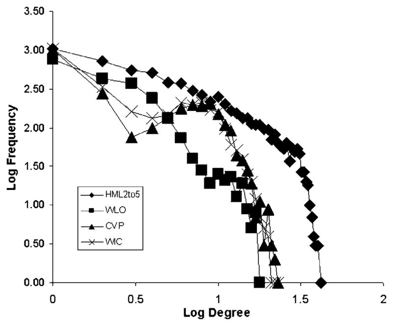
Degree distributions, showing log frequency as a function of log degree, for each of the three pseudolexicons and the HML2to5 lexicon.

Mean Shortest Path Length

The mean shortest path length is the mean, across all pairs of nodes, of the minimum number of links that must be traversed to get from one node of the pair to the other. Table 4 shows the mean shortest path length between any two nodes for each of the lexicons as calculated by the Pajek program. It makes little sense to talk about the shortest path between two nodes that are in different islands because the path length between them is infinite. Further, path lengths between pairs of nodes in a small island are necessarily short, biasing the overall mean toward a low value. Therefore, Table 4 contains data only for the largest island in each network. Also shown in Table 4 are estimates of the mean shortest path length for comparably sized (i.e., the same number of nodes and links) Erdos-Rényi graphs (MSPL_e-r) and lattice graphs (MSPL_l). In a lattice graph, a node connects to only a small number of nearest neighbors. The formula used for estimating the mean shortest path length for Erdos-Rényi graphs was as follows:

$${\text{MSPL}}_{\text{e}-\text{r}}\approx ln(\text{n})/ln({\text{k}}_{\text{mean}}),$$ (1)

where n is the number of nodes in the network and k_mean is the mean degree of the nodes in the network. The formula used for estimating the mean shortest path length for lattice graphs was as follows:

$${\text{MSPL}}_1\approx \text{n}/(2{\text{k}}_{\text{mean}}).$$ (2)

Table 4.

Mean shortest path length for each lexicon.

Path Lengths	WLO	CVP	WIC	HML2to5	HML
MSPL	7.02	5.20	5.58	5.66	6.08
E-R Expecteda	5.68	4.14	4.38	3.87	3.98
Lattice Expectedb	235	173	206	321	357

Note. MSPL = mean shortest path length.

^aExpected MSPL for an Erdos-Rényi graph with the same number of nodes as in the largest island of the indicated lexicon.

^bExpected MSPL for a lattice graph with the same number of nodes as in the largest island of the indicated lexicon.

(See Albert & Barabási, 2002, and Watts & Strogatz, 1998, for additional details.) For all the lexicons, the mean shortest path length is just slightly larger than the path length expected for an Erdos-Rényi graph and more than one and a half orders of magnitude less than the path length expected for a lattice graph. Thus, these networks all qualify for having a relatively small mean shortest path length (cf. Watts & Strogatz, 1998).

Clustering Coefficient

There are actually two measurements of clustering that have been used in the literature. What we earlier termed CCraw is simply the number of neighbor pairs formed by a node’s neighbors divided by the total possible number of neighbor pairs that could be formed by that node’s neighbors. What we refer to as CCadj (for degree-adjusted CC) is the node’s CCraw multiplied by the ratio of the node’s degree to the highest degree occurring in the network:

$$\text{CCadj}={\text{CCraw}}^{\ast }(\text{k}/{\text{k}}_{max}).$$ (3)

Because k/k_max is less than or equal to 1, CCadj for a given word is less than or equal to CCraw.

Table 5 shows the mean CCraw and the mean CCadj for the largest island of each of the lexicons. It also shows the expected CCraw for Erdos-Rényi graphs of equivalent size, referred to here as CCer (Albert & Barabási, 2002):

$$\text{CCer}\approx {\text{k}}_{\text{mean}}/\text{n},$$ (4)

where k_mean is the mean degree across all nodes in the network and n is the number of nodes in the network. As can be seen in Table 5, all the lexicons have a CCraw (and CCadj) much higher than CCer. This finding of larger than “random” CC values combined with the finding of mean shortest path lengths that are nearly as small as those expected in Erdos-Rényi graphs qualify all the lexicons as having “small-world” structures (Watts & Strogatz, 1998).

Table 5.

Mean clustering coefficients (CCs) for each lexicon.

CC Measure	WLO	CVP	WIC	HML2to5	HML
Whole lexicon
CCraw	0.196	0.216	0.199	0.278	0.219
CCadj	0.043	0.069	0.062	0.066	0.048
CCer	0.0014	0.0018	0.0016	0.0013	0.0008
Largest island
CCraw	0.239	0.276	0.248	0.296	0.283
CCadj	0.053	0.090	0.078	0.072	0.066
CCer	0.0021	0.0029	0.0024	0.0016	0.0014

Note. CCraw = unadjusted CC; CCadj = degree-adjusted CC, as explained in the text; CCer = CC expected in an equivalently sized Erdos-Rényi graph, as explained in the text.

Assortative Mixing

Finally, we computed the amount of assortative mixing in each of the lexicons. Recall that assortative mixing is a measure of whether nodes tend to have neighbors with about the same degree as their own degree. Do highly connected nodes connect to other highly connected nodes or to nodes of low degree? As a measure of assortative mixing, we used the correlation of a node’s degree with the degree of each of its neighbors. Positive assortative mixing indicates that nodes with high degrees tend to have neighbors that also have high degrees, and nodes with low degrees tend to have neighbors with low degrees. Table 6 shows the Pearson product–moment correlation of a node’s degree with its neighbors’ degrees, for each lexicon and for the largest island of each lexicon. All the lexicons show a high amount of positive assortative mixing. The amount of assortative mixing tends to be higher in the whole lexicons than in the largest islands. This result occurs because each whole lexicon contains its respective largest island along with a number of nodes of lower degree outside of that island whose neighbors are, by necessity, also of low degree. (Recall that each lexicon is comprised of one large island and a number of much smaller islands. A node’s degree can be no larger than its island size. Hence, considering nodes outside the largest island, each lexicon pairs low degree nodes with low degree nodes.) This necessary pairing of like nodes with one another tends to inflate the overall positive correlation.

Table 6.

Pearson product–moment correlations of a node’s density with the density of each of its neighbors.

Network Component	WLO	CVP	WIC	HML2to5	HML
Whole lexicon	0.608	0.519	0.541	0.635	0.663
Largest island	0.535	0.419	0.460	0.621	0.614

Summary of Results of Simulations

When modeled as a complex graph based on the single phoneme deletion, addition, or substitution rule, all three pseudolexicons examined here showed the same set of five characteristics reported by Vitevitch (2008) for the HML. First, each graph consisted of a single large island, a large number of hermits, and a large number of small islands (a mean island size on the order of two to three nodes). Second, each graph’s degree distribution was better fit by an exponential distribution than by a power law distribution, indicating that the graph is not a scale-free network that grew via preferential attachment (Albert & Barabási, 2002; Barabási & Albert, 1999). Third and fourth, each graph had a small-world structure. The mean shortest path length between any two nodes in the largest island was quite short, approaching that found in equivalently sized (in terms of the number of nodes and links) Erdos-Rényi random graphs and was certainly much smaller than that expected in equivalently sized lattice graphs. The CC, on the other hand, was large—much larger than that expected in equivalently sized Erdos-Rényi graphs. Fifth, each graph exhibited a large amount of positive assortative mixing. Nodes tended to link to other nodes with a degree similar in magnitude to their own.

Discussion and Conclusions

For all five of the graph-theoretic properties examined here, the pseudolexicons, despite their relatively small number of phonotactic constraints, showed the same qualitative pattern of results that were obtained for the full HML. Our pseudolexicons did not grow over time. Each network basically came into existence all at once. Hence, there is no need to appeal to growth processes of any kind to explain the occurrence of these five properties. Rather, they appear to be a consequence of how the graphs were constructed. A small number of “parts” (segments) was used to create a larger number of “wholes” (words) by randomly sequencing the parts. The wholes were then linked in a graph based on the overlap of parts. Considerations of parsimony would argue that the same explanation should also be applied to the occurrence of these same five properties in the HML. Hence, the occurrence in the HML of the five properties under consideration can be explained without recourse to growth processes operating either during language acquisition or during language evolution. In particular, the existence of these five properties in a network cannot be interpreted as support for the lexical restructuring hypothesis (or any other growth or developmental process), operating across either a short or long time frame.

The results of our analyses of the pseudolexicons are not a perfect quantitative match to those obtained from the HML. The pseudolexicons tended to have more hermits and smaller largest islands than did the comparably sized HML2to5. (Note, though, that in terms of this measure, as constraints are added to the pseudolexicons—that is, as we move from the WLO to the CVP to the WIC lexicons—the pseudolexicons came to more closely resemble the HML2to5.) The degree of positive assortative mixing in the HML2to5 appeared to be a bit larger than in the pseudolexicons, although it is substantial in all the lexicons. The CVP and WIC lexicons showed a dip at low degrees in the degree distribution that is not evident in the HML2to5 (or the WLO lexicon). It is possible that these small discrepancies would disappear as more and more phonotactic constraints are added to the pseudolexicons. In any case, it remains true that the pseudolexicons examined here showed the same qualitative graph-theoretic characteristics as the full HML, indicating that the qualitative pattern of results can be reproduced using minimal constraints. Additional constraints, however, may be necessary for reproducing the precise quantitative pattern of results.

Our results should not be misconstrued to imply that whenever a graph links wholes based on part overlap, these five properties will emerge. Our results do show what properties of that graph are likely to emerge, all else being equal, when parts are randomly combined into wholes. Because of its hierarchical structure, language lends itself to the construction of networks based on such part–whole relations. Phonological segments are constructed from phonetic features or from articulatory gestures. Words and syllables are constructed from segments. Words are also constructed from syllables. Sentences are constructed from words. The concepts represented by words are frequently thought of as collections of semantic features. The degree of overlap of these features between two concepts indicates the semantic similarity of those concepts. Graphs based on such part-overlap, again assuming random combinations of parts, would be expected to show the same five characteristics we observed. Deviations from such a pattern could, of course, still occur. Such a deviation would indicate a departure from randomness, and it is precisely when such a deviation occurs that a search for causes deeper than a simple random combination of parts is necessary. Our results establish the baseline necessary for identifying such deviations.

Our results also do not imply that these graph-theoretic properties have no important consequences for real-time language processing. The structure of the mental lexicon has important implications for processing information within that lexicon, as pointed out by Vitevitch (2008), regardless of how that structure came to be. A lexicon with a small-world structure allows for faster and more robust processing than a lexicon with longer paths between words. A lexicon with high positive assortative mixing can remain connected even when a highly connected node is itself lost or damaged in some way—such a network would show resistance to the damaging effects of noise and degradation. These advantages accrue regardless of the reasons the network has the structure that it does or how it evolved.

The five graph-theoretic properties examined here may have important behavioral consequences as well. A word’s degree (more frequently referred to as its neighborhood density), mean shortest path length, CC, and extent of assortative mixing may all affect how easy or difficult a word is to recognize. In fact, degree is well-known to affect ease of spoken word recognition (e.g., Luce & Pisoni, 1998). The extent to which other, more subtle structural measures (such as CC or mean shortest path length) also affect the ease with which spoken words can be recognized is just beginning to be explored. A study of the effects of phonological spread by Vitevitch (2007) is a good example. Spread refers to the number of different phoneme positions at which a word can be changed into one of its phonological neighbors. Spread and CC are closely related and may, in fact, measure the same underlying psychological construct, something akin to “neighborhood cohesion.” When neighborhood density is held constant, as a word’s spread decreases its CC increases, and as a word’s spread increases its CC decreases—as the number of positions at which a neighbor can be formed increases, the proportion of those neighbors that are themselves neighbors decreases. (If a word has a spread of 1, then all its neighbors are themselves neighbors, and the CC is 1. If the spread is equal to the word’s length, len, then the probability of any two neighbors themselves being neighbors, and hence the expected value of the CC, is 1/len.)

In three different behavioral tasks, Vitevitch showed that words with a low spread (high CC) were processed more efficiently (i.e., faster) than words with a high spread (low CC). Our hope is that additional behavioral and cognitive studies exploring the effects of such graph-theoretic measures of the mental lexicon will increase our understanding of the fundamental processes used in spoken word recognition. In the visual word recognition literature, studies of the effect of spread or CC have been used to argue for top-down feedback from the word identification level to the letter identification level (e.g., Mathey, Robert, & Zagar, 2004; Mathey & Zagar, 2000). Similarly, understanding the effects of CC may help resolve the longstanding debate concerning the existence or nonexistence of feedback from the word level to the phoneme level in models of spoken word recognition (McClelland & Elman, 1986; McClelland, Mirman, & Holt, 2006; McQueen, Norris, & Cutler, 2006; Mirman, McClelland, & Holt, 2006; Norris, McQueen, & Cutler, 2000).

The use of graph-theoretic techniques and complex networks to study language in particular and cognition more generally is a relatively new research approach (Dorogovtsev & Mendes, 2001; Ferrer i Cancho & Solé, 2001; Motter, de Moura, Lai, & Dasgupta, 2002; Soares, Corso, & Lucena, 2005; Steyvers & Tenenbaum, 2005; Wilks & Meara, 2002; Wilks, Meara, & Wolter, 2005). There is a danger that our results will be interpreted overly negatively to indicate that such endeavors are not fruitful. We neither intend such an interpretation nor believe such an interpretation to be correct. First, as just discussed, the behavioral consequences of graph-theoretic variables are unclear at this time and represent an unexplored area for future research. Second, as argued previously, it is precisely when deviations from the “random” or “no growth” pattern are found that a search for a more complex explanation is warranted. To recognize the deviations, however, we first need to know the baseline case. The present work helps us to know that baseline case. In any new area of research, it takes time to learn what the appropriate “control groups” and benchmarks are. The simulation and modeling work reported here contributes to understanding that appropriate control group for future studies of the mental lexicon and other areas of interest to students of language using graph-theoretic constructs.

Third, graph-theoretic studies can lead to new and counterintuitive hypotheses about language. Two examples may help clarify this point. Soares et al. (2005) constructed a network of Portuguese syllables based on their co-occurrence in words in the language. Two nodes (syllables) in the network were linked if they co-occurred in one or more words. The degree distribution of this network was well fit by a power law, a finding commonly interpreted to indicate that the network grew over time via preferential attachment as opposed to random growth processes (Albert & Barabási, 2002; Barabási & Albert, 1999). Soares et al. concluded that as words were added to the Portuguese language, they re-used syllables already frequently occurring in Portuguese, a somewhat counterintuitive hypothesis as it tends to maximize the perceptual confusability of new words with existing words.

As a second example, Ferrer i Cancho and Solé (2001) used a large corpus of English text to construct a network in which the nodes represented words. Two nodes were linked when the two words co-occurred at a greater than chance frequency within the corpus. This network showed a somewhat peculiar degree distribution. It was well-fit by two power laws, with different slopes, one for small degrees and one for larger degrees. In modeling this distribution using a preferential attachment–like process, Dorogovtsev and Mendes (2001) found that the bifurcated distribution was a natural consequence of their network growth (i.e., language evolution) assumptions. The two parts of the degree distribution could be naturally interpreted as corresponding to a noncore lexicon and a core or kernel lexicon, consisting of approximately 5,000 frequently used and frequently co-occurring words. Further, an implication of their model was that as the lexicon continued to grow, once the kernel lexicon was established, it (the kernel) would not change in size as words were added to the language. Hence, if new words became part of the kernel lexicon, old words already in the kernel would need to be removed. Obviously, as is always the case, converging evidence is required to confirm these hypotheses. However, these two studies do point to the ability of formal graph-theoretic analyses and associated modeling to lead to new and interesting hypotheses about language structure and processing and to bring new data to bear on existing hypotheses.

In summary, complex networks based on phonetic similarity, reflecting part (or segmental) overlap, and built from instantaneously created pseudolexicons, in which words were randomly generated from a set of segments and subjected to minimal phonotactic constraints, showed the same major structural properties as a lexical network built from actual English words. These results indicate that the emergence of those properties does not depend on processes of language (or network) evolution or acquisition, be those processes language specific or applicable to a variety of subject-matter domains. In particular, neither growth nor lexical restructuring is necessary to produce these properties. Instead, those structural properties emerge naturally when a network is built with nodes created from a relatively small set of parts, and the links between those nodes are based on the degree of overlap of those parts across the two nodes.

References

- Albert R, Barabási AL. Statistical mechanics of complex networks. Reviews of Modern Physics. 2002;74:47–97. [Google Scholar]
- Barabási A-L. Linked: The new science of networks. Cambridge, MA: Perseus; 2002. [Google Scholar]
- Barabási AL, Albert R. Emergence of scaling in random networks. Science. 1999 October 15;286:509–512. doi: 10.1126/science.286.5439.509. [DOI] [PubMed] [Google Scholar]
- Batagelj V, Mrvar A. Pajek—A program for large network analysis. Connections. 1998;21:47–57. [Google Scholar]
- Callaway DS, Hopcroft JE, Kleinberg JM, Newman MEJ, Strogatz SH. Are randomly grown graphs really random? Physical Review E. 2001;64:041902. doi: 10.1103/PhysRevE.64.041902. [DOI] [PubMed] [Google Scholar]
- Charles-Luce J, Luce PA. Similarity neighborhoods of words in young children’s lexicons. Journal of Child Language. 1990;17:205–215. doi: 10.1017/s0305000900013180. [DOI] [PubMed] [Google Scholar]
- Charles-Luce J, Luce PA. An examination of similarity neighborhoods in young children’s receptive vocabulary. Journal of Child Language. 1995;22:727–735. doi: 10.1017/s0305000900010023. [DOI] [PubMed] [Google Scholar]
- Coady JA, Aslin RN. Phonological neighborhoods in the developing lexicon. Journal of Child Language. 2003;30:441–469. [PMC free article] [PubMed] [Google Scholar]
- Dollaghan CA. Children’s phonological neighborhoods: Half empty or half full? Journal of Child Language. 1994;21:257–271. doi: 10.1017/s0305000900009260. [DOI] [PubMed] [Google Scholar]
- Dorogovtsev SN, Mendes JFF. Language as an evolving word web. Proceedings of the Royal Society of London B. 2001;268:2603–2606. doi: 10.1098/rspb.2001.1824. [DOI] [PMC free article] [PubMed] [Google Scholar]
- Erdos P, Rényi A. On the evolution of random graphs. Publication of the Mathematical Institute of the Hungarian Academy of Science. 1960;5:17–61. [Google Scholar]
- Ferrer i Cancho R, Solé RV. The small world of human language. Proceedings of the Royal Society of London B. 2001;268:2261–2265. doi: 10.1098/rspb.2001.1800. [DOI] [PMC free article] [PubMed] [Google Scholar]
- Greenberg JH, Jenkins JJ. Studies in the psychological correlates of the sound system of American English. Word. 1964;20:157–177. [Google Scholar]
- Grosjean F. Spoken word recognition processes and the gating paradigm. Perception & Psychophysics. 1980;28:267–283. doi: 10.3758/bf03204386. [DOI] [PubMed] [Google Scholar]
- Gruenenfelder TM, Mueller ST. Research on Spoken Language Processing Progress Report No. 28. Bloomington, IN: Indiana University; 2007. Power law degree distributions can fit averages of non-power law distributions. [Google Scholar]
- Harary F. Graph theory. Reading, MA: Addison-Wesley; 1969. [Google Scholar]
- Higgins PM. Nets, puzzles, and postmen: An exploration of mathematical connections. Oxford, England: Oxford University Press; 2007. [Google Scholar]
- Landauer TK, Streeter LA. Structural differences between common and rare words: Failure of equivalence assumptions for theories of word recognition. Journal of Verbal Learning and Verbal Behavior. 1973;12:119–131. [Google Scholar]
- Luce PA, Pisoni DB. Recognizing spoken words: The neighborhood activation model. Ear and Hearing. 1998;19:1–36. doi: 10.1097/00003446-199802000-00001. [DOI] [PMC free article] [PubMed] [Google Scholar]
- Mathey S, Robert C, Zagar D. Neighbourhood distribution interacts with orthographic priming in the lexical decision task. Language and Cognitive Processes. 2004;19:533–559. [Google Scholar]
- Mathey S, Zagar D. The neighborhood distribution effect in visual word recognition: Words with single and twin neighbors. Journal of Experimental Psychology: Human Perception and Performance. 2000;26:184–205. doi: 10.1037//0096-1523.26.1.184. [DOI] [PubMed] [Google Scholar]
- McClelland JL, Elman JL. The TRACE model of speech perception. Cognitive Psychology. 1986;18:1–86. doi: 10.1016/0010-0285(86)90015-0. [DOI] [PubMed] [Google Scholar]
- McClelland JL, Mirman D, Holt LL. Are there interactive processes in speech perception? Trends in Cognitive Sciences. 2006;10:364–369. doi: 10.1016/j.tics.2006.06.007. [DOI] [PMC free article] [PubMed] [Google Scholar]
- McQueen JM, Norris D, Cutler A. Are there really interactive processes in speech perception? Trends in Cognitive Sciences. 2006;12:533. doi: 10.1016/j.tics.2006.10.004. [DOI] [PubMed] [Google Scholar]
- Metsala JL. An examination of word frequency and neighborhood density in the development of spoken-word recognition. Memory & Cognition. 1997a;25:47–56. doi: 10.3758/bf03197284. [DOI] [PubMed] [Google Scholar]
- Metsala JL. Spoken word recognition in reading disabled children. Journal of Educational Psychology. 1997b;89:159–169. [Google Scholar]
- Milgram S. The small world problem. Psychology Today. 1967;2:60–67. [Google Scholar]
- Mirman D, McClelland JL, Holt LL. Response to McQueen et al.: Theoretical and empirical arguments support interactive processing. Trends in Cognitive Sciences. 2006;10:534. doi: 10.1016/j.tics.2006.06.007. [DOI] [PMC free article] [PubMed] [Google Scholar]
- Motter AE, de Moura APS, Lai YC, Dasgupta P. Topology of the conceptual network of language. Physical Review E. 2002;65(6):065102. doi: 10.1103/PhysRevE.65.065102. [DOI] [PubMed] [Google Scholar]
- Newman MEJ. Assortative mixing in networks. Physical Review Letters. 2002;89:208701. doi: 10.1103/PhysRevLett.89.208701. Available online at http://arxiv.org/abs/cond-mat/0205405. [DOI] [PubMed]
- Newman MEJ, Park J. Why social networks are different from other types of networks. Physical Review E. 2003;68:036122. doi: 10.1103/PhysRevE.68.036122. [DOI] [PubMed] [Google Scholar]
- Newman RS. The level of detail in infants’ word learning. Current Directions in Psychological Science. 2008;17:229–232. [Google Scholar]
- Norris D, McQueen JM, Cutler A. Merging information in speech recognition: Feedback is never necessary. Behavioral and Brain Sciences. 2000;23:299–370. doi: 10.1017/s0140525x00003241. [DOI] [PubMed] [Google Scholar]
- Nusbaum HC, Pisoni DB, Davis CK. Research on Speech Perception Progress Report No. 10. Bloomington, IN: Indiana University; 1984. Sizing up the Hoosier mental lexicon: Measuring the familiarity of 20,000 words. [Google Scholar]
- Pastor-Satorras R, Vespignani A. Evolution and structure of the internet. Cambridge, England: Cambridge University Press; 2004. [Google Scholar]
- Soares MM, Corso G, Lucena LS. The network of syllables in Portuguese. Physica A: Statistical Mechanics and its Applications. 2005;355:678–684. [Google Scholar]
- Steyvers M, Tenenbaum JB. The large-scale structure of semantic networks: Statistical analysis and a model of semantic growth. Cognitive Science. 2005;29:41–78. doi: 10.1207/s15516709cog2901_3. [DOI] [PubMed] [Google Scholar]
- Storkel HL. Restructuring of similarity neighborhoods in the developing mental lexicon. Journal of Child Language. 2002;29:251–274. doi: 10.1017/s0305000902005032. [DOI] [PubMed] [Google Scholar]
- Swingley D. Phonetic detail in the developing lexicon. Language and Speech. 2003;46:265–294. doi: 10.1177/00238309030460021001. [DOI] [PubMed] [Google Scholar]
- Swingley D, Aslin RN. Lexical neighborhoods and the word-form representations of 14-month-olds. Psychological Science. 2002;13:480–484. doi: 10.1111/1467-9280.00485. [DOI] [PubMed] [Google Scholar]
- Vitevitch MS. The spread of the phonological neighborhood influences spoken word recognition. Memory & Cognition. 2007;35:166–175. doi: 10.3758/bf03195952. [DOI] [PMC free article] [PubMed] [Google Scholar]
- Vitevitch MS. What can graph theory tell us about word learning and lexical retrieval? Journal of Speech, Language, and Hearing Research. 2008;51:408–422. doi: 10.1044/1092-4388(2008/030). [DOI] [PMC free article] [PubMed] [Google Scholar]
- Walley A. The role of vocabulary development in children’s spoken word recognition and segmentation ability. Developmental Review. 1993;13:286–350. [Google Scholar]
- Walley AC. Speech perception in childhood. In: Pisoni DB, Remez RE, editors. The handbook of speech perception. Malden, MA: Blackwell; 2005. pp. 449–468. [Google Scholar]
- Watts DJ, Strogatz SH. Collective dynamics of ‘small-world’ networks. Nature. 1998 June 4;393:440–442. doi: 10.1038/30918. [DOI] [PubMed] [Google Scholar]
- Webster’s Seventh Collegiate Dictionary. Los Angeles: Library Reproduction Services; 1967. [Google Scholar]
- Wilks C, Meara P. Untangling word webs: Graph theory and the notion of density in second language word association networks. Second Language Learning. 2002;18:303–324. [Google Scholar]
- Wilks C, Meara P, Wolter B. A further note on simulating word association behaviors in a second language. Second Language Learning. 2005;21:359–372. [Google Scholar]