Functional, But Not Anatomical, Separation of “What” and “When” in Prefrontal Cortex

Abstract

How does the brain store information over a short period of time? Typically, the short-term memory of items or values is thought to be stored in the persistent activity of neurons in higher cortical areas. However, the activity of these neurons often varies strongly in time, even if time is unimportant for whether or not rewards are received. To elucidate this interaction of time and memory, we reexamined the activity of neurons in the prefrontal cortex of monkeys performing a working memory task. As often observed in higher cortical areas, different neurons have highly heterogeneous patterns of activity, making interpretation of the data difficult. To overcome these problems, we developed a method that finds a new representation of the data in which heterogeneity is much reduced, and time- and memory-related activities became separate and easily interpretable. This new representation consists of a few fundamental activity components that capture 95% of the firing rate variance of >800 neurons. Surprisingly, the memory-related activity components account for <20% of this firing rate variance. The observed heterogeneity of neural responses results from random combinations of these fundamental components. Based on these components, we constructed a generative linear model of the network activity. The model suggests that the representations of time and memory are maintained by separate mechanisms, even while sharing a common anatomical substrate. Testable predictions of this hypothesis are proposed. We suggest that our method may be applied to data from other tasks in which neural responses are highly heterogeneous across neurons, and dependent on more than one variable.

Introduction

A prominent form of neural activity that occurs in the absence of external stimulation is persistent activity—often associated with the active maintenance of short-term memory information in the brain (Fuster and Alexander, 1971; Funahashi et al., 1989; Fuster, 1995; Goldman-Rakic, 1995; Miller et al., 1996; Romo et al., 1999; Averbeck and Lee, 2007). Neurophysiological experiments to investigate this phenomenon typically rely on behaviors in which a subject has been trained to remember an item for a “delay period” lasting a few seconds. On each trial of such a task, an item, which varies from trial to trial, is briefly presented to the subject, and the subject uses the memory of that item to guide action or decision making at the end of the delay period. Actions that reveal that the item was correctly held and recalled from short-term memory are then rewarded. Different experiments have used different types of items to be held in memory. Examples include the identity of an object (Fuster and Alexander, 1971), the direction of a saccade (Funahashi et al., 1989; Averbeck and Lee, 2007), the identity and/or location of a visual image (Miller et al., 1993, 1996), and the frequency of a mechanical vibration applied to a finger (Romo et al., 1999). A consistent observation has been that neural firing rates, in the prefrontal cortex (PFC) and other areas, are sensitive to the identity of the item held in memory throughout the delay period. These firing rates are therefore thought to be the neural substrate of the short-term memory required in the task.

In these experiments, neural responses exhibit an intricate and convoluted representation of information, without any obvious order on the population level. Such heterogeneity across neurons is characteristic of the PFC and greatly complicates interpretation of data, which in turn hinders the formulation of mechanistic hypotheses and testable predictions. With regards to short-term memory tasks, one perplexing issue has been that the information represented on the single neuron level is not always relevant to the task: neural activity is often sensitive to the amount of time elapsed during the delay period, even though the subject does not need to estimate the duration of the delay period to guide appropriate behavior. Some neurons may have firing rates that rise or fall as time elapses during the delay period, but most of them have complex time-dependent patterns that interact in myriad ways with the identity of the item held in memory (Kojima and Goldman-Rakic, 1982; Quintana and Fuster, 1992; Rao et al., 1997; Chafee and Goldman-Rakic, 1998; Rainer et al., 1999; Brody et al., 2003). Apparently then, the neural representation of items held in short-term memory is inextricably linked with some representation of the length of the delay period length.

These observations raise two types of questions: (1) Representation. What is the precise nature of the representations in prefrontal cortex? Given that individual neurons differ strongly in their response properties, can we find a description of their activities on the population level such that this description is easily interpretable, is stable throughout the delay period, captures all of the information represented, and generalizes easily across monkeys? (2) Mechanism. Given the dynamic, rather than static, character of short-term memory, can we construct a dynamic model of the network activity that allows us to understand the mechanistic underpinnings of the short-term storage of information in the prefrontal cortex?

Here we address these questions by analyzing a previously reported dataset collected from the PFC of monkeys (Romo et al., 1999; Brody et al., 2003; Romo and Salinas, 2003). In these experiments, the item held in memory was the frequency of a vibratory stimulus applied to a fingertip (Fig. 1A).

Figure 1.

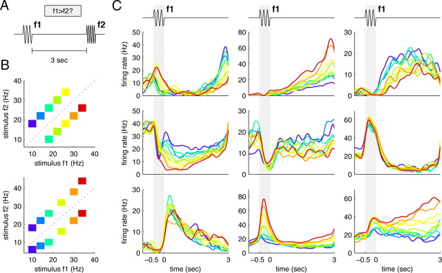
Two-interval discrimination task and example recordings from the PFC. A, Schematic diagram of the two-stimulus interval discrimination task. Two brief (0.5 s) vibratory stimuli with frequencies f1 and f2 are sequentially applied to a monkey's fingertip. The monkey needs to determine whether f1 is larger than f2, and must therefore remember the value of f1 throughout the delay period. We focus on this memory delay period in this paper. B, Typical stimulus sets used. Each box represents a particular [f1,f2] pair used in a trial. Different stimulus pairs were pseudorandomly interleaved over different trials. The colors represent the frequency of the first stimulus f1. C, Smoothed PSTHs from nine different cells from the PFC. The curves are colored according to the frequency f1 of the applied stimulus; colors are the same as in B. The neurons are but a small sample from the PFC, demonstrating some of the complexity and diversity found in the recorded activity.

Materials and Methods

Recordings and data preprocessing.

Details of the training and electrophysiological methods have been described before (Brody et al., 2003). Briefly, three monkeys (Macaca mulatta; henceforth labeled RR013, RR014, and RR015) were trained to compare and discriminate the frequencies of two mechanical vibrations presented sequentially to the fingertip (Fig. 1A. The two stimuli, frequency f1 and f2, were separated by a few seconds. The monkeys were trained on the task up to their psychophysical thresholds, with stimulus frequencies in the range 6–40 Hz, which in humans give rise to the percept known as flutter (Talbot et al., 1968). The sets of stimulus frequencies used are shown in Figure 1B, the top shows the set used for monkey RR013, the bottom the set used for monkeys RR014 and RR015.

Neurophysiological recordings began after training was complete. Single neuronal activity was recorded through seven independently movable microelectrodes (2–3 MΩ) (Romo et al., 1999; Salinas et al., 2000; Hernández et al., 2002), separated from each other by 500 μm and inserted in parallel into the inferior convexity of the PFC of the left hemisphere of the three monkeys and into the right hemisphere of two monkeys (RR013 and RR015). Results from both right and left PFCs were similar and data have been collapsed across them. Recordings sites changed from session to session. From the single-unit activity picked up by the electrodes, neurons were preselected for (weakly) task-locked activity in the following way: on each trial, the spike counts were taken during 500 ms windows (1) before the onset of stimulus f1, (2) during the presentation of stimulus f1, (3) at the beginning of the delay period, (4) at the end of the delay period, and (5) during the presentation of stimulus f2. For each combination of stimulus frequencies (f1,f2), we applied a one-way ANOVA test to the spike counts collected from these different task episodes. This procedure yielded one p value for each combination of frequencies. We included the neuron if the median of these p values was <0.01. We note that this neuron preselection step is not necessary for the analysis here, since principal component analysis (PCA) will eliminate any non-task-related activity. However, the preselection allowed us to determine approximately how many neurons with task-locked activity the dataset comprises: N = 842 cells for monkey RR013, N = 161 cells for monkey RR014, N = 361 cells for monkey RR015, and N = 123 for monkey RR013 with a 6 s delay period. After this preselection step, we focused exclusively on the delay period of each trial, during which the subject is holding the value of f1 in short-term memory.

For the data analysis, spike trains on individual trials were first filtered with a Gaussian kernel with width 50 ms and then discretized in 10 ms steps; the first 150 ms of the delay period were excluded to eliminate transient firing rate changes from the presentation of stimulus f1. For each neuron i, we therefore obtained a set of time-varying firing rates r_i^k(t, f) where k denotes the trial, t the elapsed time with respect to the onset of the delay period, and f the first stimulus frequency. For the network modeling, we used a 100 ms time step to ensure sufficient speed of the parameter-fitting procedure.

Principal component analysis.

In a first step, we sought to reduce the dimensionality of the dataset using PCA (Kantz and Schreiber, 1997). Here we provide an abbreviated technical description of the method to supplement the more intuitive explanation provided in Figure 2 and in Results. A detailed explanation of the methods used can be found in the supplemental material (available at www.jneurosci.org).

Figure 2.

Caricature of the dimensionality reduction process. A, Artificially generated firing rates for three cells during the delay period of the task. As before, colors indicate different stimuli f1. B, The firing rates can be embedded in state space, and a new coordinate system (black lines) can be found through PCA. The new coordinate system has two axes (labeled r1 and r2, respectively) that span the two-dimensional subspace in which the trajectories evolve, and a third axis (r3) that reaches into the (irrelevant) orthogonal subspace. C, Representation of the simulated data in the new coordinate system. Note that the direction of the axes is arbitrary: the first axis could also represent a linear drop in firing rates.

PCA yields a new coordinate system for a multivariate dataset such that the first coordinate accounts for as much of the variance in the data as possible, the second coordinate for as much of the remaining variance as possible, and so on. The new coordinate system is found by diagonalizing the covariance matrix of the data. Consistent with the intuition provided in Figure 2, we define the covariance matrix of the data (“signal and noise”) as follows:

where r̄_i(t, f) denotes the trial-averaged firing rate of neuron i—the smoothed peristimulus time histogram (PSTH)—and the angular brackets denote averaging over the time points, t, and the stimulus frequencies, f. The diagonalization of the covariance matrix, C = UΛU^T, yields both the eigenvalues of C in the diagonal entries of the matrix Λ, and a new coordinate system in the columns of the matrix U. We will refer to the columns of U as the principal axes of the new coordinate system. These new axes can be used to re-represent the original data. The coordinates of the data with respect to the principal axes are called the principal components and are given by the following:

The principal components are therefore linear combinations of the firing rates of the individual cells. The variance of these principal components are given by the respective eigenvalues of the covariance matrix C. For the data, the eigenvalues are shown in Figure 3, A and B (red dots), and the first six principal components are shown in Figure 3D.

Figure 3.

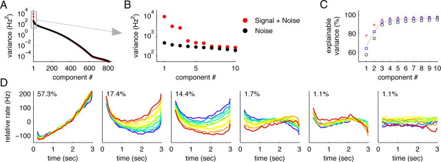
Dimensionality reduction. A, B, Eigenvalues resulting from PCA for monkey RR013 (N = 842 neurons). The red dots show the eigenvalues of the covariance matrix of the neural firing rates (“signal + noise”). The black dots show the eigenvalues of the covariance matrix if before the analysis, the trial-averaged firing rate of each neuron is subtracted (“noise”). C, Cumulative percentage of signal variance captured by the principal components. The symbols show the results for recordings from three different monkeys (black circles, RR013; blue square, RR014; red crosses, RR015), the gray line the average over the monkeys. After n = 6 dimensions, >95% of the variance is captured on average. D, Projections of the data onto the n = 6 principal axes found with PCA for monkey RR013. Percentages indicate the amount of signal variance captured by the respective principal components.

Variance in the trial-averaged firing rates r̄_i(t, f) will be both due to any task-locked changes in the firing rate and due to residual noise in the firing rate estimates. To be able to separate variance caused by task-locked activity from these other types of variance, we performed a separate PCA on estimates of the residual noise traces η̄_i(t, f). These estimates were obtained by taking differences between single-trial estimates of the firing rate:

where M denotes the number of trials, and the upper indices k and l indicate the trial. Just as with the original firing rates, we can define a covariance matrix, H, for these noise traces. The eigenvalues of this “noise” covariance matrix are also shown in Figure 3, A and B (black dots). The largest eigenvalue of H sets an upper bound to the amount of variance that could potentially be due to noise along any axes in the state space. In turn, the sum of the n largest eigenvalues of H sets an upper bound for the amount of variance that could potentially be due to noise in any n-dimensional subspace. When subtracting this number from the variance captured by the first n principal components of the original data, we obtain a lower bound on the explainable variance captured by the n-dimensional subspace (Fig. 3C). Empirically, we find that six principal axes suffice to capture >95% of the explainable variance in the data (Fig. 3). A more detailed explanation of the rationale behind this method is provided in the supplemental material (available at www.jneurosci.org).

Since cortical spike trains are approximately Poisson distributed, the variance in firing rates due to trial-to-trial variability grows linearly with the average firing rate. This could potentially lead to distortions in the results from PCA as neurons with higher firing rates contribute more to the variance than neurons with lower firing rates, even if their average firing rate does not change at all. To see whether this is a problem for our dataset, we performed an analysis that included a variance-stabilizing transformation as a preprocessing step. For that purpose, we first took the square root of all single-trial firing rates, r_i^k(t, f)→$\sqrt{r_i^k\left(t,f\right)}$. The results obtained with this preprocessing were essentially similar to those obtained without preprocessing.

Difference of covariances method.

In a second step, we sought to separate variance caused by changes in firing rates due to f1 from variance caused by changes in firing rates through time. To measure variance caused by f1, we averaged time out of the ith principal component, z̄_i(t, f), to obtain the time average z̄_i(f). Similarly, to measure variance occurring through the passage of time, we averaged over frequencies, to obtain the frequency average of the ith component, z̄_i(t). These two types of variances can then be contrasted by taking the difference of their respective covariance matrices:

To the extent that the time-dependent and frequency-dependent variances are separable, the difference matrix S will have positive eigenvalues for variance caused mostly by net changes of the firing rates through time, and negative eigenvalues for variance caused mostly by frequency dependence of the firing rates. Accordingly, the diagonalization of this matrix yields a coordinate system in which time- and frequency-dependent variance are maximally separated. Applied to the data that was preprocessed with PCA, this difference-of-covariances (DOC) method results in another six-dimensional Cartesian coordinate system that spans the same subspace as the coordinate system found through PCA. As detailed in the supplemental material (available at www.jneurosci.org), the resulting coordinate system underwent two (minor) adjustments designed to optimize the read-outs of time and frequency. We note that such a separation of time and frequency could also be obtained through an iterative combination of classical multivariate methods such as linear discriminant analysis and principal component analysis. The advantage of the DOC method we propose here is that it is simpler and more general since it directly separates the different sources of variances.

The successful separation of time and frequency variance that we report in this article is a feature of the data, rather than the DOC method. The DOC method does not guarantee such a separation, and it is fairly straightforward to design examples in which such a separation cannot succeed. We provide such an example in section 5 of the supplemental material (available at www.jneurosci.org). In this section, we also show that the main results of the DOC method hold when the initial PCA reduction step uses a different dimensionality.

Dynamical model.

Finally, we fitted a linear dynamical model to the components z̄_i(t, f) obtained from the DOC method. If we denote the dynamical variables of the model by the six-dimensional vector z(t), then the model can be written as follows:

where A is the 6 × 6 mixing matrix A and b a six-dimensional vector of external inputs. Since the frequency dependence of the firing rates is a result of the previously applied stimulus f1, we modeled this dependence by introducing frequency-dependent initial conditions, z(0) = d(f). The parameters of this model, A, b, and the initial conditions, d(f), were all estimated by minimizing the mean-square error between the dynamical model and the DOC components z̄_i(t, f) obtained from the data. The minimization of the mean-square error was performed using a conjugate gradient descent technique (Press et al., 1992). An explicit computation of the gradient, can be found in the supplemental material, available at www.jneurosci.org.

Since the number of parameters to be fitted is quite large, we added an L1-regularization term on the coefficients of the mixing matrix A (Hastie et al., 2001). The performance of the model was then evaluated using cross-validation. More specifically, the model parameters where estimated on a dataset in which one of the stimuli f was initially excluded. The predictive error of the model was then evaluated on the data from the excluded stimulus. We defined the predictive error as the mean-square error between the original DOC components and the model simulation, normalized by the signal power (see Fig. 8C). The regularization parameter was chosen so as to optimize the predictive power of the model.

Figure 8.

Network model, original data, and simulations. A, Effective network connectivity in the PFC during the delay period of the sequential discrimination task. Neurons are sorted with respect to the strength of their tuning to the stimulus f1. Neurons with similar tuning are connected through excitatory connections (red), neurons with opposite tuning through inhibitory connections (blue). B, Distribution of external inputs. C, Prediction errors of the simulated network when compared to the original data. D, Data of four neurons, replotted from Figure 1C, panels 1–4. E, Simulated neurons in the reconstructed network. The simulations reproduce key trends in the data without echoing the noise.

Results

A state-space description of the data

In the two-stimulus-interval discrimination task shown in Figure 1A, a monkey first receives a brief vibratory stimulus (with frequency f1) onto its fingertip, waits for a few seconds, receives a second vibratory stimulus (with frequency f2), and then, depending on whether f1 > f2, must press one of two pushbuttons to receive a juice reward (Romo et al., 1999). Directly after application of the stimulus f1, the monkey needs to actively remember f1 to complete the task successfully.

The required short-term memory trace of f1 is reflected in the persistent activity of neurons in the PFC (Romo et al., 1999; Brody et al., 2003), some examples of which are shown in Figure 1C.

These examples give only a glimpse of the actual complexity and diversity of neural responses during the delay period, a complexity that makes it difficult to give an adequate and complete summary of neural response properties. Here, we set out to find a compact population-level description of the data based on intuitions about the state space of neural responses as spelled out below (Kantz and Schreiber, 1997; Friedrich and Laurent, 2001).

At any given point in time, we consider the state of the network of PFC neurons to be described by the instantaneous firing rate of each of its neurons. Thus the state of a network of 800 neurons is described by 800 firing rates, a point in an 800-dimensional space. For each value of f1, as time proceeds during the delay period, the point moves through this very large space, tracing out some curve. For F different values of f1, we are therefore examining F different curves or trajectories, as shown in Figure 2B. Potentially, the state of the network could move through some lower-dimensional subspace, rather than through all 800 dimensions, and the trajectories could then be restricted to this subspace. In the diagram in Figure 2, the trajectories are confined within a two-dimensional plane and do not reach into the full three-dimensional space. Since the spread of the trajectories can be measured by their variance in different directions, a natural and commonly used choice for identifying such a potential subspace is PCA, a variance-based dimensionality reduction technique (Kantz and Schreiber, 1997). PCA will yield a new coordinate system, in which axes are ordered by the amount of variance they capture in the data. After identification of the new coordinate system, the subspace dynamics can be visualized by plotting the data with respect to the new axes (see the diagram example in Fig. 2C for illustration). For the recordings from the PFC, as will be shown below, the coordinate axes thus found do not separate time and frequency information. We used PCA as a standard preprocessing step before then attempting separation of time- and frequency-dependent information. This latter step is not achieved through PCA but through the DOC method that we develop and apply below.

Most of the variance in prefrontal cortex during short-term memory of f1 is time dependent, not f1 dependent

Do the experimentally observed firing rate states lie within a lower-dimensional subspace? Firing patterns of different neurons are found to be extremely heterogeneous (Fig. 1C), suggesting that the curves could be quite complex, perhaps erratic in shape, and that most directions in the state space could be represented. At the same time, the firing rates of each neuron in each condition change relatively smoothly in time, suggesting in contrast that a low-dimensional parameterization of the data could be found. We used PCA to quantitatively determine the dimensionality required to provide an accurate description of the data. We found that, despite the heterogeneity across neurons, as few as n = 6 dimensions, i.e., six directions in the state space, suffice to account for >95% of the explainable variance in the data (Fig. 3) (N = 842 cells in one monkey). To separate genuine variations in firing rates from those caused by noise, we performed PCA both on the trial-averaged firing rates (“signal + noise”) (Fig. 3A,B, red dots) and on estimates of the trial-to-trial variability (“noise”) (Fig. 3A,B, black dots) (see Materials and Methods). The results show a few axes along which the variance in signal and noise is much larger than the variance in noise. Subtracting the noise variance from the signal-and-noise variance yields the explainable variance, i.e., the amount of variance in the data that can be attributed to the signal. When assuming a criterion that 95% of the explainable variance should be accounted for, we found that n = 6 dimensions suffice (Fig. 3C), a significant reduction in the number of variables required to describe the data. Just as in the toy example in Figure 2, the data can subsequently be displayed with respect to the new, low-dimensional coordinate system, as shown in Figure 3D. Here, the y-axis in each panel corresponds to a principal component, i.e., the value of the data when projected onto the respective principal axis. This value is computed for each time point and each frequency f1. As in the original data, we represent time on the x-axis and color code the frequencies f1. Note that each of the principal components corresponds to one particular linear combination (weighted sum) of the firing rates of the 800 neurons.

Surprisingly, the first principal component (>57% of the explainable variance) does not contain any information about the memory of f1, but simply rises approximately linearly with time (Fig. 3D, first panel). This rise is independent of the value of f1, as seen by the close overlap of the different colored curves. This finding was unexpected because, as described in the introduction, correct behavior in this task is not defined in terms of the amount of time elapsed during the delay period, but only in terms of the values of the two stimuli, f1 and f2. Nevertheless, the data indicate that the dominant variable in the PFC during the delay period is not the value of the stimulus f1. Instead, it is time.

The remaining axes in Figure 3D, second through sixth, do capture information about f1. For example, knowing the value of the third principal component, plotted in the third panel of Figure 3D, would give an observer information about the value of the previously presented stimulus f1. However, this representation of f1 is mixed with various time dependencies: to uniquely identify f1, the observer would need to know both the value of the principal component (y-axis position) and the value of time (x-axis position). This mixing reflects the original mixing of temporal dependencies and f1 stimulus information found at the single cell level (Fig. 1).

Time and frequency information can be separated with the DOC method

While PCA allows us to reduce the dimensionality of the data, the coordinate system found by PCA, Figure 3, does not yield any particular insight into how information is represented in the PFC (except for the first axis). The definition of correct behavior on a trial (accurately answering “f1 > f2? Y or N”) tells us that, quite separately from time during the delay period, f1 is a crucial variable for the task. We therefore sought to find a coordinate system, within the six-dimensional subspace, that would separate (1) firing rate variance caused by differences of the network state due to f1, but not due to time and (2) firing rate variance caused by changes in the network state through time, but not due to differences in f1. To specifically contrast these two variables, we developed a DOC method that performs an unsupervised coordinate transformation of the data (see Materials and Methods). Our approach is thus different from alternative analyses that would not consider the nature of the behavioral task, such as applying independent component analysis to the neural firing rates (Hyvärinen et al., 2001). The DOC method, like PCA, finds axes that are orthogonal to each other which allows computing the fraction of total variance captured by each axis.

We applied the method to the six dimensions obtained by PCA, resulting in a coordinate transformation within those six dimensions that achieved an almost perfect demixing of time-dependent and f1-dependent variances (Fig. 4A). When averaged over three monkeys, >96.3 ± 2.7% (μ ± σ) of the time-dependent variance resides in the first three dimensions of the new coordinate system (Fig. 4B–D, panels 1–3, henceforth called time components) and >99.8 ± 0.2% of the f1-dependent variance resides in the last three dimensions (Fig. 4B–D, panels 4–6, henceforth called f1 components). Accordingly, the time- and f1-dependent variances split into two separate three-dimensional subspaces. Note that most of the total variance falls into the subspace of time components (82.4 ± 6.7% on average) (see also percentages shown in Fig. 4B–D), and only a smaller fraction into the subspace of f1 components (17.6 ± 6.7% on average).

Figure 4.

Separation of time and f1 variance using an additional coordinate transformation. A, The time-dependent variance (blue) and f1-dependent variance (red) for the different dimensions of the new coordinate system. The first three panels show the results for three different monkeys, the last panel the results for monkey RR013 when the delay period was doubled to 6 s. In all monkeys, there is a natural separation into two subspaces. The first subspace (dimensions 1–3) captures almost all of the time-dependent variance (>96.3%), the second subspace (dimensions 4–6) almost all of the f1-dependent variance (>99.8%). B, Data projected onto the six axes of the new coordinate system for monkey RR013 (N = 842 cells). The numbers give the percentage of the overall variance captured by each component, similar to Figure 3D. C, D, Coordinate systems found using the same analysis for two other monkeys. These results are based on N = 161 cells (monkey RR014) and N = 361 neurons (monkey RR015), respectively. E, Monkey RR013 with a 6 s delay period (N = 123 neurons). The delay period activity is approximately rescaled by a factor 1/2. B–E, Scaling of the y-axis is normalized with respect to the first panel in each row.

The new coordinate system, which is still Cartesian and covers the same subspace as the principal components of Figure 3D, is shown in Figure 4B for the same data as in Figure 3D. The axes are now ordered according to the amount of time-dependent and f1-dependent variance they capture. While the first axis yields a reliable read-out of the passage of time during the delay period, independent of the stimulus f1, the last axis (Fig. 4B, sixth panel) yields a reliable and static representation of the stimulus f1, independent of time.

Hence, even though most of the single cell firing rates mix f1 and time dependencies during the delay period, there are linear combinations of these firing rates that allow reading out time and f1 information independently of each other. However, the corresponding two dimensions (Fig. 4, first and last panels) do not capture the complete population dynamics. Rather, there are further dimensions that take part in representing information during the delay period. For instance, another time component (Fig. 4B, second panel) returns to its initial state at the end of the delay period, similar to a swing.

Quite interestingly, another f1 component (Fig. 4B, fifth panel) evolves slowly during the delay period and thereby changes the population representation of the memorized frequency f1. One possible interpretation for this change is that the system seeks to move the information about f1 into a separate memory buffer to avoid overwriting f1 when the second stimulus f2 comes in. Such a mechanism could help to solve the problem of context-dependent processing that the task requires (f1 and f2 need to be treated differently) (see also Chow et al., 2009).

Our method also allowed us to perform a quantitative comparison of PFC recordings from three different monkeys. As shown in Figure 4, C and D, the coordinate systems found with exactly the same method for the recordings from two other monkeys are quite similar (Fig. 4C,D; N = 161 cells in C; and N = 361 cells in D), even though the representational power attributed to the coordinates themselves changes somewhat. This result demonstrates that the population-level description accurately captures the representation of short-term memory information across monkeys.

We emphasize that these results are a feature of the PFC data, they are not simply a consequence of the method. We discuss this point in the supplemental material (available at www.jneurosci.org) and show a simple simulated example in which application of the DOC method yields very different results.

Information separation is functional, but not anatomical

The sharp separation between “what” and “when” information shown in Figure 4 raises the question whether there exists a similar distinction at the anatomical level. Despite the complexity of single cell responses, there could still be two categories of cells, one mostly representing time, the other mostly f1. This would lead to a corresponding, yet trivial, separation of time and f1 information at the population level. To investigate this question, we first note that the individual neuron activities can be reconstructed quite accurately as weighted sums of the six components shown in Figure 4A (see also supplemental material, available at www.jneurosci.org). Consequently, we can associate a vector of n = 6 reconstruction coefficients with each neuron. If there were separate categories of neurons, then we could expect a bimodal (or multimodal) distribution of these six-dimensional reconstruction vectors (see, for instance, Paz et al., 2005).

We tested this hypothesis by performing many random projections of the vectors into one, two, or three dimensions. However, we did not observe any evidence for separate clusters of neurons in these random projections, making it highly unlikely that such a simple clustering of cells exists (Dasgupta, 2000). Rather, the reconstruction vectors seem to be distributed according to a unimodal distribution, centered around the coordinate origin, with approximately exponential tails (Fig. 5). Consequently, the neurons in the PFC form a highly distributed representation of time and frequency information. Although time and f1 information are functionally separate, and can be read out independently of each other, they share the same anatomical substrate.

Figure 5.

No evidence for separate clusters of cells. The firing rates of every cell can be reconstructed by a linear combination of the six components from Figure 4. Every cell can therefore be represented by six parameters, its reconstruction vector. The figure shows a projection of the reconstruction vectors of all cells onto a (random) two-dimensional plane, as well as the respective marginal distributions. All such random projections yield similar results, suggesting that the vectors follow a unimodal, spherical distribution with approximately exponential tails. Consequently, no separate groups or clusters of cells could be identified.

Dynamical model suggests separate mechanisms for time and frequency dynamics

Although there is no anatomical separation of “what” and “when” information, there may still exist a separation of mechanisms at the network level. To study this possibility, we asked what minimal type of network model is needed to reproduce the observed firing rates. The simplest possible dynamical model is a linear model, so we began by exploring this possibility. Our reduction of the dimensionality to only six components in no way implies that a linear model would fit the data well. Low-dimensional dynamics can of course be highly nonlinear. For example, Hodgkin–Huxley action potential dynamics are low-dimensional yet highly nonlinear (Koch, 1999). Nonetheless, we found that the experimentally observed dynamics could be fit quite successfully with a simple linear dynamical model:

where the six-dimensional vector z(t) describes the neural firing rates in the coordinate system of Figure 4A. Note that this dynamical model provides a macroscopic description of the network dynamics using the population activities z_k(t), rather than single neuron activities; its relation to actual network models is described below. The 6 × 6 mixing matrix A captures the mutual dependencies of the dimensions, and the vector b contains possible external inputs. To fit this model to the data and obtain the mixing matrix A and the external inputs b, we used regularized gradient descent (see Materials and Methods). To run the model, we “seed” it at time step t = 0 with initial z values obtained from the fit. Iterative application of the update rule (Eq. 6) then produces the model data for subsequent time steps. The resulting simulations closely match the experimental data (compare Fig. 7A with Fig. 4B).

Figure 7.

Simulation of the linear dynamical model and rescaling of time. A, The simulated traces of the linear dynamical model, Equation 6, closely match the original data, Figure 4B. B, Simulation after the off-diagonal 3 × 3 blocks of the mixing matrix A have been set to zero. C, Simulation of the same system over a 6 s delay period. D, Simulation over a 6 s after the external inputs have been rescaled by half, and the 3 × 3 diagonal matrix for the f1 component has been adjusted.

The mixing matrix A and the external inputs b are shown in Figure 6, A and B. Most of the off-diagonal entries in the mixing matrix are zero (or close to zero), and only a few are large enough to influence the system behavior. The separation of the time- and f1-dependent subspaces is reflected by a similar decoupling of their dynamics: the weights between time components (dimensions 1–3) and f1 components (dimensions 4–6) are negligible (see off-diagonal 3 × 3 blocks in Fig. 6a). Consequently, when setting these elements to zero, the simulation of the system does not change significantly (Fig. 7B). In addition, there is another distinction between the two subspaces, concerning the external inputs: Whereas the time components receive strong external drives (Fig. 6B), the f1 components receive only negligible external inputs.

Figure 6.

The linear dynamical model. A, The mixing matrix A of the model, as estimated from the data of monkey RR013. B, The external inputs b of the model, as estimated from the same data. Note that the time components (1–3) are driven by strong external inputs, whereas the frequency components (4–6) are not.

In sum, despite the lack of an anatomical separation of “what” and “when” information, our model shows that the mechanisms underlying the time dependence and the f1 dependence of the neural activities may very well be separable and independent of each other. This is done by an effective decoupling of the respective dynamics in which the time components are driven by external inputs, whereas the f1 components are driven by their mutual dependencies in the mixing matrix A.

A network model of short-term memory

The construction of the dynamical model on the population level can finally be inverted to yield an entire network model of the data in which, neuron-by-neuron, the delay period firing rates from the original dataset are reproduced (Fig. 8). Using neurons with linear input–output relations, we used the following equation:

where W is the connectivity of the network and E are the external background inputs. Both W and E can be determined from the parameters of the linear dynamical model, A and b (see supplemental material, available at www.jneurosci.org). Since the network model is deterministic, it does not reproduce the “noise” or trial-to-trial variability in the original recordings. It does, however, capture the dynamics of each cell quite well, with prediction errors rarely exceeding 10% of the explainable variance (Fig. 8C).

The resulting network connectivity and external inputs are shown in Figure 8, A and B. To display the connectivity matrix W, we sorted the neurons by the slope of their f1-tuning curves during the delay period. Most of the neuron-to-neuron connectivities are close to zero, but neurons with similar tuning usually excite each other (red areas on the upper left and lower right) and neurons with opposite tuning usually inhibit each other (blue areas on the lower left and upper right). When neurons are sorted according to their time dependence (e.g., ramping up versus ramping down), the connectivity matrix acquires a similar structure (data not shown), reflecting the highly distributed nature of the population representations. Even though the time components can now be controlled through the external inputs E, and the f1 components through changes in the recurrent connectivity W, there is no unique anatomical correlate of this separation at the level of individual cells or individual synapses between cells.

Rescaling of time and model predictions

The separation of f1 (“what”) and time (“when”) in Figure 4 shows that distinct representations of these two variables can be found in the population activity of prefrontal neurons. The generative model of Figure 7 further suggests that this separation is not merely a matter of data analysis, but may correspond to a separation of mechanisms in the brain. If the mechanisms maintaining the representation of time and those maintaining the representation of f1 are indeed separate, we should be able to affect one but not the other. We therefore considered the effects of manipulating time separately from manipulating f1.

One manipulation that treats the time-dependent and f1-dependent aspects of the task differently is to change the duration of the delay period without changing the value of the f1 or f2 stimuli nor the nature of the task. Thus the timing of the task is affected, but the sensory stimuli f1 remain exactly the same. This manipulation was performed in a subset of the original experimental runs when the data were collected (Brody et al., 2003). The majority of the data were collected using a standard 3 s delay period, as we have used in most of the analysis in this paper. But some neurons were also recorded during blocks of trials with a 6 s delay period. It was found that, after the monkeys had been accustomed to the new delay period length, the main effect of doubling the duration of the delay period was to slow down the dynamics of the changes in firing rates by a factor of 1/2 [compare Brody et al. (2003), their Fig. 8]. Consistent with this finding, our analysis, applied to this separate set of data (N = 123 neurons, monkey RR013), yielded components (Fig. 4E, with a 6 s time axis) that are approximately rescaled versions of the original components (Fig. 4B, with a 3 s time axis).

How can such a rescaling be implemented in our generative model? This is seen most easily for the component that accounts for the most variance, component 1. The activity of this component is an almost perfectly straight ramp in time (Fig. 4A, leftmost panel). Correspondingly, this first component has a self-weight almost exactly equal to 1, a strong constant external input, and no significant connections from other components of the model (Fig. 6A,B). Component 1 thus acts as an almost perfect integrator of its constant external input. The strength of its external input determines the rate at which component 1 changes with time. In fact, this characteristic holds approximately for all three time components, and their dynamics can be accelerated or decelerated simply by increasing or decreasing the strength of their external drive (compare Fig. 7C,D, panels 1–3).

In contrast, the f1 components have negligible external drives (Fig. 6B). This includes component 5 in which the dynamics of individual trajectories is determined by the strength of the self-connection weights within the f1-dependent group, not by the strength of an external input. Rescaling the time axis of these dynamics therefore requires a change in connectivity strength, not merely a change in external input. Halving the cross-connection weights correspondingly leads to the correct rescaling (compare Fig. 7C,D, panels 4–6).

Thus, a direct implication of our generative model of the prefrontal network is that time rescaling of time components requires only a change in external inputs; in contrast, time rescaling of the f1 components requires changes in the recurrent synaptic connections within the network. Changes in external inputs can generally be much faster than changes in synaptic connection strength. Laboratory long-term potentiation induction protocols, for example, often require many repeated trials and take place over minutes (Caporale and Dan, 2008). Given these differences, our model predicts that on switching from a familiar 3 s delay period block to an also familiar but now 6 s delay period block of trials, rescaling of the time components could be done much faster than rescaling of the f1 components. During the first few trials after a switch, inadequate f1 rescaling would lead to degraded accuracy in the memory of f1—that is, the subjects' representation of what is being held in memory would be impaired, slowly regaining its normal accuracy as the f1 rescaling is completed. In contrast, we hypothesize that changes in external inputs could be very rapid, from one trial to the next. Thus the subjects' estimate of when the delay period will end could adapt very rapidly, regaining its normal accuracy within only one or two trials of a switch into a familiar block of long delay period trials.

These contrasting predictions for when and what follow from the separation of mechanisms suggested by the generative model, Equation 6. We must note that the contrasting predictions depend on the assumption that the requisite changes in synaptic connectivity strengths are slow, on the order of minutes or longer; this assumption could be wrong. The predicted effects would be observable, and therefore testable, at both the behavioral and neurophysiological level. However, they would be best observed near behavioral psychometric threshold (value of f1 close to value of f2), where slight impairments in the accuracy of the remembered f1 would be most noticeable.

Discussion

The large heterogeneity of responses in higher cortical areas makes it difficult to understand neural activity on the population level. We here focused on a particular problem, that of short-term memory, in which neurons in PFC often have persistent firing rates that carry information about an item in short-term memory, yet also vary strongly in time. Our main aim in this study was to elucidate this interaction of time and memory information. In particular, we asked how information about time and memory are represented in PFC and what type of mechanisms may underlie such a representation.

To address our first question, that of representation, we searched for a reduced-dimensionality representation of the data in which time and frequency dependence of the neural firing rates could be separated. Our analysis began with a PCA preprocessing step that shows that as few as six dimensions capture most (>95%) of the explainable variance in the firing rates of a large set of cells. Given the prominent heterogeneity of neural responses, this was not a foregone conclusion from the PCA analysis, but is instead a feature of our particular dataset. For example, if each neuron fired at a high rate at a single moment during the delay period, with different neurons firing at different times, as found during singing in area HVC of songbirds (Hahnloser et al., 2002), or as found in hippocampus of rats trained to estimate the duration of a delay period (Pastalkova et al., 2008), the number of dimensions could not have been reduced at all.

However, while PCA served to summarize the data, most of the coordinates found did not reveal a useful representation of the data (Fig. 3). For that purpose, we developed the DOC method, which yielded a much more easily interpretable representation and revealed essentially complete separability of the time-dependent and f1-dependent variations in the firing rates (Fig. 4A). This functional separation exists at the population level, not at the single neuron level. Functional separability of time and f1 components had previously been postulated in a theoretical model of the delay period data (Singh and Eliasmith, 2006). Our analysis of the experimental data confirms this postulate. Intriguingly, the analysis also shows that, unlike the Singh and Eliasmith model, in which there was only one time component and one f1 component, there are at least three time and three f1 components in the data.

Based on the novel DOC representation, and to address our second question, that of mechanism, we then constructed a dynamical network model that replicates many details of the data. Even though the individual neurons within the resulting network mix time and f1 information just as the actually recorded neurons, their activities are produced from an underlying population representation in which time and f1 do not interact. A key aspect of the model was that the underlying time- and f1-dependent dynamics are driven by separate mechanisms: the representation of time is largely driven by external inputs into the network, while that of f1 is largely driven by internal recurrent connectivity.

The model could, perhaps, be interpreted merely as a compact summary of the dynamics in the data. However, we propose a stronger interpretation. That is, we propose to interpret the network mechanisms that maintain the time and f1 representations in the model as suggesting characteristics of the biological network mechanisms. Thus, we take our model to suggest that the biological mechanisms underlying the time dependence and the f1 dependence of the data are in fact functionally separate, with time representation relying mostly on external inputs, while the f1 representation relies mostly on internal recurrent connectivity. In this view, the basic principles of models previously proposed for the short-term memory of f1 and its comparison to f2 (Miller et al., 2003; Machens et al., 2005; Miller and Wang, 2006; Machens and Brody, 2008), in which temporal variation during the delay period was not addressed, may therefore still apply for the f1 components, even though the actual network implementations in the older models are too simplistic.

We used our dynamical model to generate predictions with which to test the hypothesis that time- and f1-dependent components of the neural activity are supported by separate mechanisms. Specifically, the model predicts that time-dependent components could adapt much more rapidly than f1-dependent components, both in terms of neural firing rates and in terms of behavior. These predictions can be tested experimentally.

One intriguing aspect of our results is that the dynamics in the data could be well described by a linear system. This was surprising: although the transformation from the original data to our six new axes was linear, the dynamics and state space trajectories within these new axes were neither constrained nor expected to be linear. In fact, as mentioned above, past explorations of PCA in neural population recordings have often led to low-dimensional, yet complex nonlinear dynamics (Friedrich and Laurent, 2001; Stopfer et al., 2003; Yu et al., 2006). Nevertheless, we found that here the dynamics could be summarized by a simple linear dynamical system. While this was convenient (construction of a generative model was straightforward), we do not propose that PFC, in general, is a linear system: linear systems have very limited computational power. Our proposal that the PFC acts as a linear system is limited to the delay period in this task. We speculate that the slow, linear dynamics observed during the delay period are, in fact, a signature of a (high-dimensional) continuous attractor on which the network is moving. Linear, “integrator”-like behavior is a well known computational regime of continuous attractor networks. Since continuous attractors are usually located at bifurcation points of dynamical systems, any perturbation, for instance, through sensory input, will automatically push the system into a different dynamical regime (Machens et al., 2005). We suggest that the observed linear dynamics during the delay period correspond merely to a reorganization of the stored information within a high-dimensional continuous attractor network whose computational power emerges through its sensitivity to internal and external influences. The stored information may need reorganization to prepare the system for the incoming second stimulus. PFC may seek to move the memory of f1 into a separate short-term memory buffer that will remain unaffected by the second stimulus f2.

In sum, the most important result of applying the DOC method is that it provided a view of apparently very complex data in which the underlying dynamics become transparent. Without this transparency, the hypothesis of a separation between the mechanisms supporting time representation and those supporting frequency representation would not have been formulated. Regardless of whether the hypothesis ultimately proves correct or incorrect, the DOC method gave us a tool to move our thinking forward. In this sense, the specifics of some of the results (e.g., there are three time components and three frequency components, as opposed to two and four, or four and two, respectively) are far less important than the fact that it led directly to a mechanistic, testable, hypothesis. This can be contrasted with using the PCA approach alone, which often results in complex trajectories in state space (Friedrich and Laurent, 2001; Yu et al., 2006) that allow no straightforward interpretation and lead to no specific mechanistic hypothesis. We note that some important qualitative conclusions are possible without the mechanistic models. For example, without the DOC method, and assuming only that neural activity in PFC is sufficient for the monkeys to perform the task at a variety of delay periods, it follows that there must be some time-invariant representation of f1. However, our analysis added much more than this conclusion alone: it led to specific hypotheses as to what this f1 representation is, what the mechanisms supporting it are, and how these hypotheses can be tested.

Dimensionality reduction methods serve to summarize complex data. They do not necessarily reveal new aspects of the data, but they can be helpful in doing so. With the help of an additional unsupervised coordinate transform, the DOC method, we were here able to simplify our view of the data to a point that allowed us to break down what appears to be a single problem into smaller, separable, and therefore more easily understandable problems. While related methods have been used in other neurophysiological settings (Friedrich and Laurent, 2001; Stopfer et al., 2003; Paz et al., 2005; Yu et al., 2006, 2009; Narayanan and Laubach, 2009), our findings increase the enthusiasm with which we encourage application of these methods to data from the frontal lobes. We emphasize that such separability is not guaranteed by the method, it needs to be present in the dataset. Nevertheless, multiplexed representations, where multiple variables affect the firing rates of single neurons, are often found in frontal cortices. For instance, neurons in the PFC can represent both an objects' location and its identity, suggesting that PFC integrates these two types of information (Rao et al., 1997). It would be interesting to see whether on the population level the information can be separated again. This dataset and many others may be amenable to a functional separation analysis similar to the one we have presented here.

References

- Averbeck BB, Lee D. Prefrontal neural correlates of memory for sequences. J Neurosci. 2007;27:2204–2211. doi: 10.1523/JNEUROSCI.4483-06.2007. [DOI] [PMC free article] [PubMed] [Google Scholar]
- Brody CD, Hernández A, Zainos A, Romo R. Timing and neural encoding of somatosensory parametric working memory in macaque prefrontal cortex. Cereb Cortex. 2003;13:1196–1207. doi: 10.1093/cercor/bhg100. [DOI] [PubMed] [Google Scholar]
- Caporale N, Dan Y. Spike timing-dependent plasticity: a Hebbian learning rule. Annu Rev Neurosci. 2008;31:25–46. doi: 10.1146/annurev.neuro.31.060407.125639. [DOI] [PubMed] [Google Scholar]
- Chafee MV, Goldman-Rakic PS. Matching patterns of activity in primate prefrontal area 8a and parietal area 7ip neurons during a spatial working memory task. J Neurophysiol. 1998;79:2919–2940. doi: 10.1152/jn.1998.79.6.2919. [DOI] [PubMed] [Google Scholar]
- Chow SS, Romo R, Brody CD. Context-dependent modulation of functional connectivity: secondary somatosensory cortex to prefrontal cortex connections in two-stimulus-interval discrimination tasks. J Neurosci. 2009;29:7238–7245. doi: 10.1523/JNEUROSCI.4856-08.2009. [DOI] [PMC free article] [PubMed] [Google Scholar]
- Dasgupta S. Experiments with random projection. Proceedings of the 16th Conference on Uncertainty in Artificial Intelligence; San Francisco: Kaufmann; 2000. pp. 143–151. [Google Scholar]
- Friedrich RW, Laurent G. Dynamic optimization of odor representations by slow temporal patterning of mitral cell activity. Science. 2001;291:889–894. doi: 10.1126/science.291.5505.889. [DOI] [PubMed] [Google Scholar]
- Funahashi S, Bruce CJ, Goldman-Rakic PS. Mnemonic coding of visual space in the monkey's dorsolateral prefrontal cortex. J Neurophysiol. 1989;61:331–349. doi: 10.1152/jn.1989.61.2.331. [DOI] [PubMed] [Google Scholar]
- Fuster JM. Cambridge, MA: MIT; 1995. Memory in the cerebral cortex. [Google Scholar]
- Fuster JM, Alexander GE. Neuron activity related to short-term memory. Science. 1971;173:652–654. doi: 10.1126/science.173.3997.652. [DOI] [PubMed] [Google Scholar]
- Goldman-Rakic PS. Cellular basis of working-memory. Neuron. 1995;14:477–485. doi: 10.1016/0896-6273(95)90304-6. [DOI] [PubMed] [Google Scholar]
- Hahnloser RH, Kozhevnikov AA, Fee MS. An ultra-sparse code underlies the generation of neural sequences in a songbird. Nature. 2002;419:65–70. doi: 10.1038/nature00974. [DOI] [PubMed] [Google Scholar]
- Hastie T, Tibshirani R, Friedman J. New York: Springer; 2001. The elements of statistical learning theory. [Google Scholar]
- Hernández A, Zainos A, Romo R. Temporal evolution of a decision-making process in medial premotor cortex. Neuron. 2002;33:959–972. doi: 10.1016/s0896-6273(02)00613-x. [DOI] [PubMed] [Google Scholar]
- Hyvärinen A, Karhunen J, Oja E. New York: Wiley Interscience; 2001. Independent component analysis. [Google Scholar]
- Kantz H, Schreiber T. Cambridge, UK: Cambridge UP; 1997. Nonlinear time series analysis. [Google Scholar]
- Koch C. Oxford, UK: Oxford UP; 1999. Biophysics of computation. [Google Scholar]
- Kojima S, Goldman-Rakic PS. Delay-period activity of prefrontal neurons in rhesus monkeys performing delayed response. Brain Res. 1982;248:43–49. doi: 10.1016/0006-8993(82)91145-3. [DOI] [PubMed] [Google Scholar]
- Machens CK, Brody CD. Design of continuous attractor networks with monotonic tuning using a symmetry principle. Neural Comput. 2008;20:452–485. doi: 10.1162/neco.2007.07-06-297. [DOI] [PubMed] [Google Scholar]
- Machens CK, Romo R, Brody CD. Flexible control of mutual inhibition: a neural model of two-interval discrimination. Science. 2005;307:1121–1124. doi: 10.1126/science.1104171. [DOI] [PubMed] [Google Scholar]
- Miller EK, Li L, Desimone R. Activity of neurons in anterior inferior temporal cortex during a short-term memory task. J Neurosci. 1993;13:1460–1478. doi: 10.1523/JNEUROSCI.13-04-01460.1993. [DOI] [PMC free article] [PubMed] [Google Scholar]
- Miller EK, Erickson CA, Desimone R. Neural mechanisms of visual working memory in prefrontal cortex of the macaque. J Neurosci. 1996;16:5154–5167. doi: 10.1523/JNEUROSCI.16-16-05154.1996. [DOI] [PMC free article] [PubMed] [Google Scholar]
- Miller P, Wang XJ. Inhibitory control by an integral feedback signal in prefrontal cortex: a model of discrimination between sequential stimuli. Proc Natl Acad Sci U S A. 2006;103:201–206. doi: 10.1073/pnas.0508072103. [DOI] [PMC free article] [PubMed] [Google Scholar]
- Miller P, Brody CD, Romo R, Wang XJ. A recurrent network model of somatosensory parametric working memory in the prefrontal cortex. Cereb Cortex. 2003;13:1208–1218. doi: 10.1093/cercor/bhg101. [DOI] [PMC free article] [PubMed] [Google Scholar]
- Narayanan NS, Laubach M. Delay activity in rodent frontal cortex during a simple reaction time task. J Neurophysiol. 2009;101:2859–2871. doi: 10.1152/jn.90615.2008. [DOI] [PMC free article] [PubMed] [Google Scholar]
- Pastalkova E, Itskov V, Amarasingham A, Buzsáki G. Internally generated cell assembly sequences in the rat hippocampus. Science. 2008;321:1322–1327. doi: 10.1126/science.1159775. [DOI] [PMC free article] [PubMed] [Google Scholar]
- Paz R, Natan C, Boraud T, Bergman H, Vaadia E. Emerging patterns of neuronal responses in supplementary and primary motor areas during sensorimotor adaptation. J Neurosci. 2005;25:10941–10951. doi: 10.1523/JNEUROSCI.0164-05.2005. [DOI] [PMC free article] [PubMed] [Google Scholar]
- Press WH, Teukolsky SA, Vetterling WT, Flannery BP. Cambridge, UK: Cambridge UP; 1992. Numerical recipes in C. [Google Scholar]
- Quintana J, Fuster JM. Mnemonic and predictive functions of cortical neurons in a memory task. Neuroreport. 1992;3:721–724. doi: 10.1097/00001756-199208000-00018. [DOI] [PubMed] [Google Scholar]
- Rainer G, Rao SC, Miller EK. Prospective coding for objects in primate prefrontal cortex. J Neurosci. 1999;19:5493–5505. doi: 10.1523/JNEUROSCI.19-13-05493.1999. [DOI] [PMC free article] [PubMed] [Google Scholar]
- Rao SC, Rainer G, Miller EK. Integration of what and where in the primate prefrontal cortex. Science. 1997;276:821–824. doi: 10.1126/science.276.5313.821. [DOI] [PubMed] [Google Scholar]
- Romo R, Salinas E. Flutter discrimination: neural codes, perception, memory and decision making. Nat Rev Neurosci. 2003;4:203–218. doi: 10.1038/nrn1058. [DOI] [PubMed] [Google Scholar]
- Romo R, Brody CD, Hernández A, Lemus L. Neuronal correlates of parametric working memory in the prefrontal cortex. Nature. 1999;399:470–473. doi: 10.1038/20939. [DOI] [PubMed] [Google Scholar]
- Salinas E, Hernández A, Zainos A, Romo R. Periodicity and firing rate as candidate neural codes for the frequency of vibrotactile stimuli. J Neurosci. 2000;20:5503–5515. doi: 10.1523/JNEUROSCI.20-14-05503.2000. [DOI] [PMC free article] [PubMed] [Google Scholar]
- Singh R, Eliasmith C. Higher-dimensional neurons explain the tuning and dynamics of working memory cells. J Neurosci. 2006;26:3667–3678. doi: 10.1523/JNEUROSCI.4864-05.2006. [DOI] [PMC free article] [PubMed] [Google Scholar]
- Stopfer M, Jayaraman V, Laurent G. Intensity versus identity coding in an olfactory system. Neuron. 2003;39:991–1004. doi: 10.1016/j.neuron.2003.08.011. [DOI] [PubMed] [Google Scholar]
- Talbot WH, Darian-Smith I, Kornhuber HH, Mountcastle VB. Sense of flutter-vibration – comparison of human capacity with response patterns of mechanoreceptive afferents from monkey hand. J Neurophysiol. 1968;31:301–334. doi: 10.1152/jn.1968.31.2.301. [DOI] [PubMed] [Google Scholar]
- Yu BM, Afshar A, Santhanam G, Ryu SI, Shenoy KV, Sahani M. Extracting dynamical structure embedded in neural activity. In: Weiss Y, Schölkopf B, Platt J, editors. Advances in neural information processing systems. Vol 18. Cambridge, MA: MIT; 2006. pp. 1545–1552. [Google Scholar]
- Yu BM, Cunningham JP, Santhanam G, Ryu SI, Shenoy KV, Sahani M. Gaussian-process factor analysis for low-dimensional single-trial analysis of neural population activity. J Neurophysiol. 2009;102:614–635. doi: 10.1152/jn.90941.2008. [DOI] [PMC free article] [PubMed] [Google Scholar]