Energy variational analysis of ions in water and channels: Field theory for primitive models of complex ionic fluids

Abstract

Ionic solutions are mixtures of interacting anions and cations. They hardly resemble dilute gases of uncharged noninteracting point particles described in elementary textbooks. Biological and electrochemical solutions have many components that interact strongly as they flow in concentrated environments near electrodes, ion channels, or active sites of enzymes. Interactions in concentrated environments help determine the characteristic properties of electrodes, enzymes, and ion channels. Flows are driven by a combination of electrical and chemical potentials that depend on the charges, concentrations, and sizes of all ions, not just the same type of ion. We use a variational method EnVarA (energy variational analysis) that combines Hamilton’s least action and Rayleigh’s dissipation principles to create a variational field theory that includes flow, friction, and complex structure with physical boundary conditions. EnVarA optimizes both the action integral functional of classical mechanics and the dissipation functional. These functionals can include entropy and dissipation as well as potential energy. The stationary point of the action is determined with respect to the trajectory of particles. The stationary point of the dissipation is determined with respect to rate functions (such as velocity). Both variations are written in one Eulerian (laboratory) framework. In variational analysis, an “extra layer” of mathematics is used to derive partial differential equations. Energies and dissipations of different components are combined in EnVarA and Euler–Lagrange equations are then derived. These partial differential equations are the unique consequence of the contributions of individual components. The form and parameters of the partial differential equations are determined by algebra without additional physical content or assumptions. The partial differential equations of mixtures automatically combine physical properties of individual (unmixed) components. If a new component is added to the energy or dissipation, the Euler–Lagrange equations change form and interaction terms appear without additional adjustable parameters. EnVarA has previously been used to compute properties of liquid crystals, polymer fluids, and electrorheological fluids containing solid balls and charged oil droplets that fission and fuse. Here we apply EnVarA to the primitive model of electrolytes in which ions are spheres in a frictional dielectric. The resulting Euler–Lagrange equations include electrostatics and diffusion and friction. They are a time dependent generalization of the Poisson–Nernst–Planck equations of semiconductors, electrochemistry, and molecular biophysics. They include the finite diameter of ions. The EnVarA treatment is applied to ions next to a charged wall, where layering is observed. Applied to an ion channel, EnVarA calculates a quick transient pile-up of electric charge, transient and steady flow through the channel, stationary “binding” in the channel, and the eventual accumulation of salts in “unstirred layers” near channels. EnVarA treats electrolytes in a unified way as complex rather than simple fluids. Ad hoc descriptions of interactions and flow have been used in many areas of science to deal with the nonideal properties of electrolytes. It seems likely that the variational treatment can simplify, unify, and perhaps derive and improve those descriptions.

INTRODUCTION

Variational methods that generalize and optimize energy functionals allow understanding of complex fluids.^{1, 2, 3, 4} Variational methods deal successfully with magnetohydrodynamics systems,⁵ liquid crystals, polymeric fluids,⁶ colloids and suspensions,^{1, 7} and electrorheological fluids.^{8, 9} Variational methods describe solid balls in liquids, deformable electrolyte droplets that fission and fuse,^{1, 10} and suspensions of ellipsoids, including the interfacial properties of these complex mixtures, such as surface tension and the Marangoni effects of “oil on water” and “tears of wine.”^{1, 7, 11}

Solid charged spheres such as sodium and chloride ions in water seemed to be a simpler fluid than deformable fissioning droplets (in some respects) and so we wondered if energy variational methods could help us understand these ionic solutions. We try to create a field theory of ionic solutions that uses only a few fixed parameters to calculate most properties in flow and in traditional thermodynamic equilibrium, both in bulk and in spatially complex domains like pores in channel proteins. We derive the differential equations of the field theory from an energetic variational principle EnVarA (energy variational analysis). Ionic solutions are often highly concentrated and so packing effects not present in infinitely dilute solutions are significant and can in fact dominate.^{12, 13, 14, 15, 16, 17, 18, 19} Interactions in concentrated environments are responsible for essential characteristics of electrodes, enzymes, and ion channels.

Our variational principle combines the maximum dissipation principle (for long time dynamics) and least action principle (for intrinsic and short time dynamics) into a force balance law that expands the law of conservation of momentum to include dissipation, using the generalized forces in the variational formulation of mechanics (p. 19 of Ref. 20, see Refs. ^{21, 22}). This procedure is a modern reworking of Rayleigh’s dissipation principle—Eq. (26) of Ref. 24—motivated by Onsager’s treatment of dissipation.^{25, 26} Our procedure optimizes both the action functional (integral) of classical mechanics^{20, 27, 28} and the dissipation functional.²⁹ The stationary point of the action is determined with respect to the trajectory of particles. The stationary point of the dissipation is determined with respect to rate functions (such as velocity). Both are written in Eulerian (laboratory) coordinates. These functionals can include entropy and dissipation as well as potential energy, and can be described in many forms on many scales from molecular dynamics calculations of atomic motion, to Monte Carlo (MC) simulations^{30, 31, 32} to—more practically—continuum descriptions^{1, 2} of ions in water. We use a primitive model^{33, 34, 35, 36, 37, 38} of ions in an implicit solvent^{39, 40, 41} and adopt self-consistent treatments of electrodiffusion^{42, 43, 44, 45, 46, 47, 48} in which the charge on ions help create their own electric field. We introduce the repulsion energy of solid spheres.^{14, 15, 17, 19, 49, 50, 51, 52} In this way, the variational calculus extends the primitive model to spatially complex, nonequilibrium time dependent situations, creating a field theory of ionic solutions.

Energy functional integrals and dissipation functional integrals are written from specific models of the assumed physics of a multicomponent system, as did Refs. ^{1, 2, 8, 9, 10}. Components of the potential energy and dissipation functions are chosen so the variational procedure produces the drift diffusion equations of semiconductor physics,^{42, 43, 44, 53} called the Vlasov equations in plasma physics,⁵⁴ or the similar biophysical Poisson–Nernst–Planck equations—named PNP by Ref. 45—and used since then by many channologists^{46, 47, 55, 56, 57, 58, 59, 60, 61, 62, 63} and physical chemists.^{48, 64} The energy of the repulsion of solid spheres is included in our functional as (1) Lennard-Jones forces^{2, 8} giving (as their Euler–Lagrange equations) a generalization of PNP for solid ions or as (2) that of uncharged spheres in the density functional theory of fluids^{58, 65, 66, 67, 68} with similar but not identical results. Boundary conditions tell how energy and matter flow into the system and from phase to phase and are described by a separate variational treatment of the “interfacial” energy and dissipation. The resulting Euler–Lagrange equations are the boundary value problems of our field theory of ionic solutions. They are derived by algebra and solved by mathematics—without additional physical approximations—in spatially complex domains, that perhaps produce flow of nonideal mixtures of ions in solution.

Ionic solutions do not resemble the ideal solutions of elementary textbooks. Indeed, ions such as Na⁺ and K⁺ have specific properties, and can be selected by biological systems, because they are nonideal and have highly correlated behavior. Screening⁶⁹ and finite size effects^{33, 34, 35, 37, 38, 70} produce the correlations more than anything else. Solvent effects enter (mostly) through the dielectric coefficient. Ionic solutions do not resemble a perfect gas⁷¹ of noninteracting uncharged particles. Indeed, because of screening,^{69, 72} the activity (which is a measure of the free energy) of an ionic solution is not an additive function as concentration is changed (Fig. 3.6 of Ref. 37; Fig. 4.2.1 of Ref. 38) and so does not easily fit some definitions (p. 6 of the book of international standards for physical chemistry⁷³) of an extensive quantity.

Some correlations are included explicitly in our models as forces or energies that depend on the location of two particles. Other correlations are implicit and arise automatically as a mathematical consequence of optimizing the functionals even if the models used in the functionals do not contain explicit interactions of components. Kirchoff’s current law (that implies perfect correlation in the flux of electrical charge⁷⁴) arises this way as a consequence of Maxwell’s equations⁷⁵ and does not need to be written separately. Variational analysis produces “optimal” estimates of the correlations that arise from those interactions^{76, 77, 78} (and p. 11 of Biot;²¹ p. 42 of Gelfand and Fromin²²) and gives the hope that fewer parameters can be used to describe a system than in models³⁴ and equations of state^{79, 80, 81} of ionic solutions which involve many parameters. These parameters change with conditions and are really functions or even functionals of all the properties of the system. (It is important to understand that in general these coupling parameters need to depend on the type and concentration of all ions, not just the pair of ions that are coupled.)

Nonideal properties are evident in all properties of ionic mixtures and most properties of ionic solutions relevant to biology and electrochemistry. Indeed, nonideal properties are responsible for the defining characteristics of many biological and electrochemical systems of great practical importance. Nonideal properties have been investigated by a generation of chemists and include (much of) the lifework of Mayer,⁸² Barthel,^{35, 83, 84} Friedman,⁸⁵ Hansen,^{12, 86} Henderson,^{87, 88} Pitzer,^{34, 70} Lee,^{33, 38} and many others.^{36, 37, 89, 90, 91, 92} Nonideal solutions require Onsager reciprocal relations^{93, 94} with parameters that depend on the type and concentration of all ions. Models of forces between atoms in molecular dynamics⁹⁵ are calibrated for the most part under ideal conditions of infinite dilution and so do not include (for the most part) the complex effects of concentration found in measurements of mixtures (see Ref. 96 and references cited there).

EnVarA does not produce a single boundary value problem or field equation for ionic solutions. Rather, it produces different field equations for different models (of correlations produced by screening or finite size, for example) to be checked by experiment. If a new component is added to the energy or dissipation functionals, the resulting Euler–Lagrange equations change form so that the solutions of the equations reflect all the interactions of the new and old components of the energy without introducing parameters (besides those in the model of the energies and dissipations themselves). Of course, the variational approach can only reveal correlations arising from the physics and components that the functional actually includes. Correlations arising from other components or physics need other models and will lead to other differential equations. For example, ionic interactions that arise from changes in the structure of water would be an example of “other physics,” requiring another model, if they could not be described comfortably by a change in the diffusion coefficient of an ion or a change in the dielectric constant of water. Numerical predictions ofEnVarA will be relatively insensitive to the choice of description (of pairwise interactions, for example) because the variational process in general produces the optimal result^{21, 22, 76, 78} for each version of the model. (This is an important practical advantage of the variational approach: compare the success of the variational density functional theory of fluids^{58, 66, 67, 68} with the nonvariational mean spherical approximation^{35, 36, 37, 38, 90, 91, 97, 98, 99, 100} that uses much the same physics.)

All field equations arising from EnVarA optimize both the dissipation and the action integrals. Inadequate functionals can be corrected (to some extent) by adjusting parameters in the functional. Effective parameters are almost always used to describe complex interactions of ions in electrolyte solutions,^{34, 70, 90, 92, 93, 100, 101, 102, 103, 104} e.g., the cross coupling Onsager coefficients^{93, 94} or Maxwell–Stefan coefficients.^{104, 105} Our work could be extended by inverse methods^{55, 106} to provide estimators¹⁰⁷ of the parameters of EnVarA functionals with least variance or bias, or other desired characteristics.

Our field theory EnVarA represents an ionic solution as a mixture of two fluids,¹⁰⁸ a solvent water phase and an ionic phase. The ionic phase is a primitive model of ionic solutions.^{35, 36, 37, 38, 90, 97, 98, 99} It is a compressible plasma made of charged solid (nearly hard) spheres. The ionic “primitive phase” is itself a composite of two scales, a macroscopic compressible fluid and an atomic scale plasma of solid spheres in a frictional dielectric. Channel proteins are described by primitive (“reduced”) models similar to those used to analyze the selectivity of calcium and sodium channels^{14, 15, 17, 18, 19, 52, 109, 110, 111, 112} and to guide the construction (using the techniques of molecular biology) of a real calcium channel protein in the laboratory.^{50, 113} Similar models predicted complex and subtle properties of the RyR channel before experiments were done in >100 solutions and in seven mutations, some drastic, removing nearly all permanent charge from the “active site” of the channel.^{51, 77, 114, 115, 116}

This paper is organized into a (1) biological introduction, (2) a theoretical introduction, (3) a long theoretical section with numbered subsections for clarity in navigation, (4) a computational methods section, (5) results, and (6) discussion. The introductions are more complete than customary as we reach to disparate communities of scientists. We try not to mystify anyone anywhere and regret that we are likely to patronize (and irritate) everyone, somewhere.

BIOLOGICAL SETTING

One of our motivations is biological. The role of ions has been a central topic in medicine and biology^{117, 118} since (at least) Fick (a biologist, actually a physiologist^{119, 120}) described diffusion. The interacting flows of ions produce the ATP (adenosine-5^′-triphosphate) (from photosynthesis and oxidative phosphorylation) that fuel life.¹¹⁷ Interacting flows of ions produce the volume regulation that allows animal cells to exist.¹²¹ Flows of ions (and their interactions) produce signaling in the nervous system, initiation of contraction in muscle, including the coordination of contraction that allows the heart to function as a pump, movement of water into the kidney and out of the stomach and intestine.¹¹⁸ Nearly all biological processes depend on ions. Biophysical chemists^{39, 122, 123} and molecular biologists^{39, 41, 124} have long dreamed that a physical theory of ions near and in proteins could provide decisive help in understanding biological function.

Biological cells, proteins, and nucleic acids are found in solutions that are plasmas of ions—ultrafiltrates of blood created by the sieving action of macroscopic pores between the cells that form capillaries. Ions in water can be called “the liquid of life” with more color than hyperbole. Ions of the biological plasma surround and pervade the proteins and nucleic acids inside a cell and inside its organelles. Ions are extraordinarily concentrated inside crevices and channels in proteins where much of their function is thought to occur in “active sites.” Concentrations are 20 M or more in the active sites of proteins and selectivity filters of channels, and nearly as large around the double helix of DNA. (Pure water has number density [H₂O]≈55 M.)

Biological plasmas outside cells are mostly sodium (∼140 mM) and chloride (∼102 mM) and bicarbonate ions (∼20 mM) mixed with small but important concentrations of potassium (∼4 mM) and calcium and magnesium ions (∼1 mM). Different ions carry different “messages” through different channels selective to one type of ion or another. The selectivity of channels for ions is a subject of the greatest biological importance. Hundreds of selective channels are described in the four “Ion Channel Fact Books.”¹²⁵

Ionic solutions inside cells are rich in potassium (∼120 mM) and chloride and organic anions (∼105 mM), with smaller concentrations of sodium (∼15 mM) and bicarbonate ions (∼25 mM) and with trace (<10⁻⁶ M) concentrations of calcium and other messenger molecules. Trace concentrations (typically <1 μM) of ions [e.g., calcium, cyclic AMP (3^′-5^′-cyclic adenosine monophosphate), inositol-tris-phosphate, even sodium] are signals that act as messengers to control many biochemical systems within cells.¹²⁶ Some important ionic messengers act in concentrations of ∼10⁻¹¹ M.¹²⁷ Measurements, simulations, and theories of such a range of concentrations are hard to perform and even harder to calibrate.

The gradient of concentration between the inside and outside of cells is a crucial energy source for the membrane phenomena that control a wide range of biological functions, as are gradients of concentrations across the membranes of many intracellular organelles. Ion concentrations inside cells are controlled by biological (nano) valves called ion channels¹²⁰ and controlled and maintained by ion transporters (“pumps”^{118, 128}) as ions move in pores within proteins across otherwise impermeable lipid membranes. It is surprising, but true, that many complex properties of channels selective for calcium or sodium ions can be understood^{14, 15, 16, 17, 18, 19, 49, 50, 51, 52, 58, 60, 67, 68, 77, 109, 110, 111, 112, 113, 114, 115, 129, 130, 131, 132, 133} using adaptations of the primitive model of ions in bulk solutions^{35, 36, 37, 38, 90, 98, 99} fulfilling the early dreams of biophysical chemists, to some extent.

In these reduced models of selectivity, the channel protein enters in a crucial but limited way. The protein contributes no mechanical or chemical energy to the ions inside it (in the simplest version of these models, however, see Ref. 110). The protein determines the size and shape of the pore in which ions are confined. It determines the mechanical and dielectric environment (i.e., the polarization charge) in and around the pore, and it provides side chains (of the amino acids that form the polypeptide backbone of the protein) that mix with the ions and water in a crowded mixture (∼20 M) in the pore of the channel. The side chains are often acidic (i.e., have permanent negative charge) or basic (i.e., have permanent positive charge), creating electric fields of great strength (∼5×10⁷ V m⁻¹). The location of the side chains in these models is an output of the calculations;⁵² they are not kept at preordained positions in a binding site, for example, because the computed positions change importantly as experimental conditions are changed. The structure of the side chains in these models is their computed positions. The structure is self-organized and the side chains have an induced fit to the mobile ions and vice versa.

The competition between electrostatic forces and crowding (produced by the finite size of the ions and the comparable size of the confining space) can be simulated by classical (originally Metropolis) MC methods developed to study bulk solutions^{98, 134, 135} or by quite approximate theories of bulk solutions,^{19, 110} or by the ad hoc but powerful density functional theory (DFT) of fluids applied to ion channels^{51, 58, 67, 68, 114, 131, 136, 137, 138} which is quite different^{137, 138, 139, 140, 141, 142} from the better known density functional theory of electrons in orbitals.

These simulations and theories of simple models of ions in crowded confined spaces allow understanding of one of the most important properties of proteins, selectivity, because they compute the nonideal properties of ions that depend on screening, the finite size of the ion, the shape and size of the confining space, and on the concentration of all species of ions.^{33, 35, 37, 38, 70} The quite different sodium channels of nerve and calcium channels of the heart are both described well by a single model with the same two fixed parameters in a wide range of solutions of different composition and content.^{15, 112, 133} Each channel type is represented only by spheres taking the place of its characteristic amino acid side chains that produce selectivity^{143, 144} (Glu Glu Glu Glu for calcium channels; Asp Glu Lys Ala for sodium channels). The simulations are confined to thermodynamic equilibrium, where there are no flows of any kind. The model is subject to all sorts of appropriate objections mostly because of its evident lack of the atomic detail of the protein. The simulations are surprisingly successful, nonetheless.^{15, 52, 112} Reduced models seem to describe the kinds of energy used by these channels to create selectivity, probably because they allow the concentrations of every ionic species to change the activity (i.e., free energy per mole) of every other ion. Of course, evolution is likely to use other forms of energy as well in other situations.

One of the Nobel Laureates who founded molecular biology (Aaron Klug) recently said, “There is only one word that matters in biology, and that is specificity. The truth is in the details, not the broad sweeps,”¹⁴⁵ reiterating the common view that selectivity can only be understood in atomic detail. The reduced model of selectivity shows that the broad sweeps of physics (in MC simulations of thermodynamic equilibrium) can compute the biological detail, at least in these calcium and sodium channels at equilibrium.

Variational analysis can extend these equilibrium simulations to nonequilibrium so they can predict current flow, creating a field theory using the same physics. EnVarA automatically calculates the time dependence of currents as the solution of its Euler–Lagrange equations. Of course, channel proteins use specialized structures to produce time dependence, the phenomena called “gating,”¹²⁰and these will not be described by EnVarA unless those structures and their energies are explicitly included in the calculations.

THEORETICAL SETTING

In this paper, we only use an energy variational analysis distinct from other variational principles¹⁴⁶ that have been used to analyze the Vlasov equation in general or at thermodynamic equilibrium (the Poisson–Boltzmann equation¹⁴⁷).

The energy variational treatment of complex fluids^{8, 9, 10} starts with the energy dissipation law,

$$\frac{dE}{dt}+\Delta =0,$$ (1)

where we use the dissipation function Δ of Onsager,²⁹ which usually includes a linear combination of the squares of various rate functions (such as velocity, rate of strain, etc).

In a classical Hamiltonian conservative system, the energy E is the sum of kinetic and internal energies involving an integral of the energy of individual particles over all space,

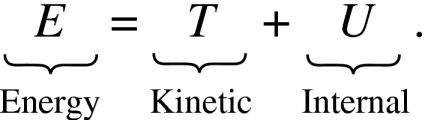(2)

The Lagrangian framework of mechanics^{20, 27, 28} writes the energy of a set of i particles in terms of the motion $\vec{\mathit{x}}\left(\vec{\mathit{X}},t\right)$ of these particles using the action $\mathsf{A}\left(\vec{\mathit{x}}\left(\vec{\mathit{X}},t\right)\right)$ of these trajectories. The i particles are labeled by the set of their initial locations $\vec{\mathit{X}}=\left\{X_i\right\}$ at t=0.

The first steps of the Legendre transformation¹⁴⁸ (pp. 32–39 of Ref. 149) give the action of the trajectories of the particles described by Eq. 2 in terms of the trajectories $\vec{\mathit{x}}\left(\vec{\mathit{X}},t\right)$,

$$\mathsf{A}=\int \left(T-U\right)dt.$$ (3)

The principle of least action optimizes the action A with respect to all trajectories $\vec{\mathit{x}}\left(\vec{\mathit{X}},t\right)$ by setting to zero the variation with respect to $\vec{\mathit{x}}$, computed over the entire domain Ω,

$$\delta \mathsf{A}={\delta }_{\vec{\mathit{x}}}\mathsf{A}={\delta }_{\vec{\mathit{x}}}\mathsf{A}\left(\vec{\mathit{x}}\right)=\int {\int }_{{\Omega }_0}\left[\mathbf{C}\mathbf{o}\mathbf{n}\mathbf{s}\mathbf{e}\mathbf{r}\mathbf{v}\mathbf{a}\mathbf{t}\mathbf{i}\mathbf{v}\mathbf{e}\mathbf{F}\mathbf{o}\mathbf{r}\mathbf{c}\mathbf{e}\right]\cdot \delta \vec{\mathit{x}}d\vec{\mathit{X}}dt,$$ (4)

where Ω₀ is the reference domain of Ω.

If ${\delta }_{\vec{\mathit{x}}}\mathsf{A}$ is set to zero, this Eq. 4 becomes the weak variation form^{29, 150} of the conservative force balance equation of classical Hamiltonian mechanics, a statement of the conservation of momentum. We use the word “force” in the generalized¹¹ sense of classical Hamiltonian mechanics (p. 19 of Refs. ^{20, 21}) and extend the classical treatment to include dissipation^{20, 21, 27} and then later to microscopic scales [Eq. 8] so we can deal with the transport energy of ions in ionic channels.

Dissipation will be treated by extending the classical treatment of the Hamiltonian to include dissipation forces.^{20, 27} When classical mechanics adds dissipation into Eq. 2 by the Rayleigh dissipation principle,^{20, 21} the physical meaning of the left hand side of Eq. 1 changes. The system is no longer conservative. It is no longer a system constrained to thermodynamic equilibrium. Confusion in the names and physical meaning of variables is likely to result (see pp. 62 and 64 of the classical textbook²⁰).

We treat dissipation by performing a variation with respect to the velocity $\vec{\mathit{u}}$ in Eulerian (laboratory) coordinates as

$${\delta }_{\vec{\mathit{u}}}\left(\frac{1}{2}\Delta \right)={\int }_{\Omega }\left[\mathbf{D}\mathbf{i}\mathbf{s}\mathbf{s}\mathbf{i}\mathbf{p}\mathbf{a}\mathbf{t}\mathbf{i}\mathbf{v}\mathbf{e}\mathbf{F}\mathbf{o}\mathbf{r}\mathbf{c}\mathbf{e}\right]\cdot \delta \vec{\mathit{u}}d\vec{\mathit{x}}.$$ (5)

If ${\delta }_{\vec{\mathit{u}}}\left(\frac{1}{2}\Delta \right)$ is set to zero, Eq. 5 gives a weak variational form of the dissipative force balance law equivalent to conservation of momentum, using the word force to include the variation of dissipation with respect to velocity. The velocity is sometimes written more explicitly as

$$\vec{\mathit{u}}\left(\vec{\mathit{x}}\left(\vec{\mathit{X}},t\right);t\right)=\frac{\partial \vec{\mathit{x}}\left(\vec{\mathit{X}},t\right)}{\partial t}=\dot{\vec{\mathit{x}}}\left(\vec{\mathit{X}},t\right).$$ (6)

Ionic solutions satisfy both dissipative force balance and conservative force balance, so we have the following equation, which can be written in either Lagrangian coordinate $\vec{\mathit{X}}$ or Eulerian coordinate $\vec{\mathit{x}}$:¹⁵¹

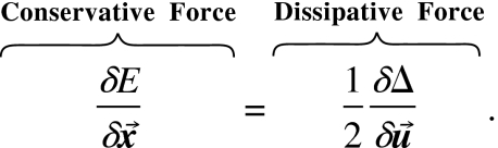(7)

One can imagine systems constrained to follow other balance “laws” beyond those in Eq. 7. Such constraints can be included in our variational analysis essentially by adding them into Eq. 7, because the theory of optimal control (Ref. 78 and p. 42 of Ref. 22) uses the variational calculus to apply constraints or penalty functions (p. 120 of Ref. 76). See discussion below, a few paragraphs before Eq. 19.

Equation 7 is nearly identical to Eq. 26 of Rayleigh.²⁴ We go beyond Rayleigh by actually solving the resulting Euler–Lagrange partial differential equations, together with the physical boundary conditions. We use the modern theory of the calculus of variations and corresponding numerical algorithms that reflect the underlying variational structures, all implemented by computational resources not available in the 19th century. Our dissipation function (like Biot’s²¹) departs from Onsager’s—loosely defined between Eqs. 5.6 and 5.7 on p. 2227 of Ref. 26—because we use variations with respect to two functions.^{29, 150} The dissipative—Onsager(ian)—part of the expression uses a variation with respect to the rate function (velocity $\vec{\mathit{u}}$).²⁹ The conservative—Hamilton(ian)—part of the expression uses a variation with respect to position $\vec{\mathit{x}}$. The combined results should be expressed in the same coordinate, either Lagrangian coordinates or Eulerian coordinates. A “pushforward” or “pullback” change of variables¹⁵¹ may be needed to write all the physical quantities in the same coordinate, if those quantities were originally defined in different coordinates.

Theoretical model: Transport of ions

The transport of ions through ionic channels is an atomic scale problem, because the diameter of channels is only 2–4× the diameters of ions. Valves like ion channels are designed to be much smaller than the systems they control. Biology carries this “to the limit” by making its nanovalves into picochannels with internal diameters about twice as large as the flowing molecules (atoms). A stochastic analysis of the trajectories of atoms is possible^{152, 153} and a multidimensional (nonequilibrium) Fokker–Planck equation can be derived by analysis⁵⁹ or steepest descent arguments.¹⁵⁴ The multidimensional Fokker–Planck equation can be reduced¹⁵⁵ to the PNP equations by a closure procedure^{59, 156, 157} with no more (than the considerable) arbitrariness of closures of equilibrium systems^{32, 158} (which do not form obviously convergent or uniformly convergent series, for example, and thus have unknown errors). The Fokker–Planck equation includes the continuity equation and so does its derivates, the drift diffusion or PNP equation. EnVarA of transport starts with an energy law that can be derived from treatments of Brownian motion, as just mentioned, but we prefer an axiomatic approach—guess the law; check the result—in which we treat Eq. 7 as a postulate, valid on the macro-, meso-, and atomic scale for two reasons: (1) present treatments of closure do not allow estimates of their errors and (2) the actual dynamics of charged particles in water and protein channels may not be well described⁵⁶ by models of the Brownian motion of uncharged particles with independent noise sources, although this has been the custom for some time.¹⁵⁹ Fluctuations in the number density of ions are likely to produce fluctuating forces not included in the treatment of Brownian motion of uncharged particles.

Theoretical model: Energy variational derivation of the Fokker–Planck equation of transport

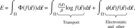
We define a generalized potential $\Phi \left(f\left(\vec{\mathit{x}}\right)\right)$ for the probability density function $f\left(\vec{\mathit{x}}\right)$ of ions and assume that electrodiffusion of particles is only driven by gradients of

(8)

where $\psi \left(\vec{\mathit{x}}\right)$ includes both the electrostatic potential $\varphi \left(\vec{\mathit{x}}\right)$ and also the steric repulsion arising from the finite volume of solid ions [see Eqs. 24, 25, 26, 27] and $\Phi \left(f\left(\vec{\mathit{x}}\right)\right)$ includes logarithmic entropy terms; β=1∕k_BT where T is the absolute temperature and k_B is the Boltzmann constant. Both electrostatic and steric repulsion forces are global forces depending on boundary conditions, the location of particles everywhere, and spatial variation of parameters like dielectric coefficients. In general, neither force can be written as functions of the position of only two particles.^{4, 69, 155} When the potential $\psi \left(\vec{\mathit{x}}\right)$ is only electrostatic $\psi \left(\vec{\mathit{x}}\right)=\varphi \left(\vec{\mathit{x}}\right)$, then $\Phi \left(f\left(\vec{\mathit{x}}\right)\right)$ describes the transport properties of an ideal gas of point charges (including screening) often described by the drift diffusion, Vlasov, or PNP equations, as mentioned previously. Even in this case, without finite size effects, the system is highly nonideal and hardly extensive since screening produces powerful correlations. The excess free energy per mole varies (more or less) as the square root of the concentration and not linearly as assumed in the “independence principle” of classical electrophysiology.¹⁶⁰

Now, we take the variation of the potential $\Phi \left(f\left(\vec{\mathit{x}}\right)\right)$ with respect to $\vec{\mathit{x}}$, in the Eulerian coordinate. Since the potential $\Phi \left(f\left(\vec{\mathit{x}}\right)\right)$ is a functional of f, not $\vec{\mathit{x}}$, we need to use the chain rule if we want to determine the spatial variation of the potential and thus the force. We write the chain rule here—only for motivation—as if variations were derivatives,

$$\frac{\delta }{\delta \vec{\mathit{x}}}\Phi \left(f\left(\vec{\mathit{x}}\right)\right)=\frac{\delta }{\delta f}\Phi \left(f\left(\vec{\mathit{x}}\right)\right)\cdot \frac{\delta }{\delta \vec{\mathit{x}}}f\left(\vec{\mathit{x}}\right).$$

The variation of $\Phi \left(f\left(\vec{\mathit{x}}\right)\right)$ with respect to $f\left(\vec{\mathit{x}}\right)$ is

$$\delta E\left(f\left(\vec{\mathit{x}}\right)\right)={\delta }_{f}E\left(f\left(\vec{\mathit{x}}\right)\right)={\int }_{\Omega }\frac{\partial \Phi \left(f\left(\vec{\mathit{x}}\right)\right)}{\partial f\left(\vec{\mathit{x}}\right)}\delta f\left(\vec{\mathit{x}}\right)d\vec{\mathit{x}}={\int }_{\Omega }\mu \delta f\left(\vec{\mathit{x}}\right)d\vec{\mathit{x}},$$ (9)

where the chemical potential μ appears because it is the derivative of $\Phi \left(f\left(\vec{\mathit{x}}\right)\right)$ with respect to density $f\left(\vec{\mathit{x}}\right)$,

$$\mu \left(f\left(\vec{\mathit{x}}\right)\right)=\frac{\partial }{\partial f\left(\vec{\mathit{x}}\right)}\Phi \left(f\left(\vec{\mathit{x}}\right)\right).$$ (10)

We introduce the flux $\vec{J}$ by its definition,

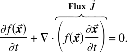(11)

Flux $\vec{J}$ is the product of density and the velocity and is the variation of the density $f\left(\vec{\mathit{x}}\right)$ with respect to $\vec{\mathit{x}}$, i.e., $\delta f\left(\vec{\mathit{x}}\right)=-\nabla \cdot \left(f\left(\vec{\mathit{x}}\right)\delta \vec{\mathit{x}}\right)$. Substitute this variation into Eq. 9, and integrate by parts, to get

$$\delta E\left(f\left(\vec{\mathit{x}}\right)\right)={\delta }_{f}E\left(f\left(\vec{\mathit{x}}\right)\right)={\int }_{\Omega }f\left(\vec{\mathit{x}}\right)\nabla \mu \left(\vec{\mathit{x}}\right)\cdot \delta \vec{\mathit{x}}d\vec{\mathit{x}}.$$ (12)

The long time dynamics are governed by the transport force $f\left(\vec{\mathit{x}}\right)\nabla \mu \left(\vec{\mathit{x}}\right)$ and the transport law. At long times, the velocity is proportional to force, and the divergence of flux is equal to the time rate of change of contents,

$$\frac{\partial f\left(\vec{\mathit{x}}\right)}{\partial t}=-\xi \nabla \cdot {\vec{J}}_f=\xi \nabla \cdot \left(f\left(\vec{\mathit{x}}\right)\nabla \mu \left(\vec{\mathit{x}}\right)\right),$$ (13)

where ξ is a renormalized constant. Equation 13 seems to be a nonlinear equation, but in fact, a little algebra shows that it is the Fokker–Planck equation,^{3, 153} describing the diffusion and drift of stochastic trajectories of density $f\left(\vec{\mathit{x}}\right)$,

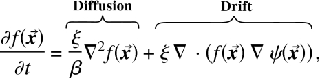(14)

where ∇² is the Laplace operator.

Equation 14 is the field equation of ionic transport on the micro (i.e., atomic) scale and $f\left(\vec{\mathit{x}}\right)$ is actually a distribution function, i.e., a probability density function that may not have been normalized.^{59, 152, 153} Later we will create a more complete model of the ionic phase by combining the atomic scale description of transport [as the drift diffusion process of Eq. 14] with a macroscopic description of the flow of a compressible ionic fluid (as a Navier–Stokes process), thereby generalizing the traditional primitive model of ionic solutions into a field theory.

Equation 13 is now written as a variation ${\delta }_{\vec{\mathit{x}}}\Phi \left(f\left(\vec{\mathit{x}}\right)\right)$ with a procedure used often in variational analysis. This procedure shows that Eq. 13 is also a dissipation—a time derivative. First, we multiply Eq. 13 by $\partial \Phi \left(f\left(\vec{\mathit{x}}\right)\right)∕\partial f=\mu \left(\vec{\mathit{x}}\right)$, and integrate,

$${\int }_{\Omega }\frac{\partial \Phi \left(f\left(\vec{\mathit{x}}\right)\right)}{\partial f\left(\vec{\mathit{x}}\right)}\frac{\partial f\left(\vec{\mathit{x}}\right)}{\partial t}d\vec{\mathit{x}}=\xi {\int }_{\Omega }\mu \left(\vec{\mathit{x}}\right)\nabla \cdot \left(f\left(\vec{\mathit{x}}\right)\nabla \mu \left(\vec{\mathit{x}}\right)\right)d\vec{\mathit{x}}.$$ (15)

Apply the chain rule to the left hand side and integrate by parts (using the chain rule in the form given on p. 220 of Ref. 28),

$${\int }_{\Omega }\frac{\partial \Phi \left(f\left(\vec{\mathit{x}}\right)\right)}{\partial t}d\vec{\mathit{x}}=-\xi {\int }_{\Omega }\left(\nabla \mu \left(\vec{\mathit{x}}\right)\right)\cdot \left(f\left(\vec{\mathit{x}}\right)\nabla \mu \left(\vec{\mathit{x}}\right)\right)d\vec{\mathit{x}}=-\xi {\int }_{\Omega }f\left(\vec{\mathit{x}}\right){\left|\nabla \mu \left(\vec{\mathit{x}}\right)\right|}^{2}d\vec{\mathit{x}}.$$ (16)

Equation 16 is the transport dissipation equal to both the conservative and dissipative terms of Eq. 7,

$$\frac{d}{dt}{\int }_{\Omega }\Phi \left(f\right)d\vec{\mathit{x}}=-\xi {\int }_{\Omega }f{\left|\nabla \mu \right|}^{2}d\vec{\mathit{x}}=\text{Transport}\text{Dissipation}.$$ (17)

This equation is a special form of Eq. 1, see Ref. 161. An explicit treatment of this atomic scale model follows to give integro-differential equations for a PNP-like system of hard spheres [see Eqs. 30, 31, 32].

Theoretical model: Primitive model as a complex fluid

We now treat the entire ionic solution in the spirit of the primitive model but as a complex composite fluid. One component is a macroscopic fluid phase—a purely macroscopic version of the primitive model of ionic solutions. Another component is a plasma, an atomic scale version of the primitive model, in which ions are represented on an atomic scale as charged Lennard-Jones spheres in a frictional dielectric. The excluded volume of the spheres can be handled on the macroscopic scale or the atomic scale. The third component is an incompressible fluid, namely, the solvent (water). Our variational approach can use more realistic models of the solvent and ion—such as density functional theory of solutions^{51, 58, 67, 68, 114, 131, 136, 137, 138}—and extend them to nonequilibrium conditions. Our approach yields multifaceted correlations without invoking complex laws with many parameters.^{34, 70, 79, 80, 81, 92, 100, 101, 102, 104, 105, 162} (Of course, the variational principle might not compute all the correlations that actually occur in the real world, if it uses a description of the energy or dissipation of the system which has inadequate resolution or is otherwise incorrect or incomplete.)

Theoretical model: Primitive ion phase, derivation, and remarks on multiscales in EnVarA

The density of spheres is variable in the primitive model and the potential of the entire primitive phase of our composite model (macroscopic and atomic) is written in the Eulerian framework before it is substituted into energy dissipation principle Eq. 1,

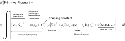(18)

where ρ_IP is the mass density, $\frac{1}{2}{\rho }_{IP}{\left|{\vec{\mathit{u}}}_{IP}\right|}^2$ is the hydrodynamic kinetic energy of the Ionic (primitive) Phase, w(ρ_IP) is the hydrodynamic potential energy, ε is the dielectric constant (dimensionless), and λ is the coupling constant (coupling scales and physical processes, as we shall see). It is the ratio of hydrodynamic (macroscopic) energy [see Eq. 3] to microscopic (atomic) energy [see Eq. 8] and has the role of a Lagrange multiplier. In general, λ must be determined by specific measurements in experiments, as has been done in rheology.^{10, 163} In special cases, λ turns out to have a specific physical meaning, e.g., as a surface tension in the theory of liquid interfaces.^{1, 164} Extensive discussion of the hydrodynamic term of Eq. 18 is found in Refs. ^{3, 165}. The solid sphere term was first used by Ref. 9, as far as we know.

Variational analysis on the macroscopic (fluid dynamics) and atomic (microscopic) scales.

Combining the macroscopic and atomic energies as we have here, using just one coordinate $\vec{\mathit{x}}$, is a drastic simplification not used in more complete and sophisticated multiscale analyses,^{3, 6} see, for example, the “micro-macro” variational analysis³² where the transformation of scales is done explicitly, with two different coordinates, one, say ${\vec{\mathit{y}}}_1$ for the macroscopic scale, and the other, say ${\vec{\mathit{y}}}_2$ for the atomic scale. In the full micro-macro expression that then takes the place of our Eq. 18 an extra nested integral$\int \cdots d{\vec{\mathit{y}}}_2$ would appear, because an integration must be done over the atomic scale ${\vec{\mathit{y}}}_2$before the energies of the atomic (microscopic) and macroscopic (hydrodynamic) scales can be combined. In the present paper we identify both the macroscopic and atomic coordinates ${\vec{\mathit{y}}}_1$ and ${\vec{\mathit{y}}}_2$ as the mesoscopic variable $\vec{\mathit{x}}$. Treatments of solution flow (i.e., solvent plus solute as needed in the study of fluid flow in the kidney, for example118), or coupled transport of ions in channels (as needed in the study of active transport by protein pumps^{118, 128}), may require a more complete micro∕macro analysis that does this integration explicitly. Our use of the density functional expression for the energy of uncharged hard spheres in Appendix C deals partially with the multiscale problem because it uses nonlocal interactions. Actually performing the integrations over both ${\vec{\mathit{y}}}_1$ and ${\vec{\mathit{y}}}_2$ is likely to do even better.

Equation 18 states the physics of our EnVarA analysis of ions in solutions and channels. In the present analysis, the hydrodynamic scale contributes only energy; no entropy terms are involved. The atomic scale, however, contributes both energy and entropy terms. The latter entropy term reflects the thermal fluctuation and the particle Brownian motion. The entropy term in Eq. 18 is on the macroscopic scale $\vec{\mathit{x}}$ and represents a crude averaging of the energetic consequences of Brownian motion (that occurs on an atomic scale ${\vec{\mathit{y}}}_2$ not shown here). A full micro-macro treatment would produce much more complete (but complex) results by explicitly averaging of the Brownian trajectories (e.g., as attempted in Refs. ^{59, 157, 166}). A full micro-macro treatment can embed MC simulations^{30, 31, 32}—perhaps even of ions in channels^{17, 112}—in the variational integral itself, i.e., as part of the integrand in Eq. 18. The variational approach was used previously in Refs. ^{167, 168}. A reduced variational approach that inspired ours is used in Ref. 169. The underlying mathematics has been summarized.²³ Simplified approaches using a single coordinate like our Eq. 18 have been published.^{170, 171} Full micro-macro analyses are available for polymeric fluids,^{3, 6} electrokinetic fluids,^{167, 168} and liquid crystals¹⁷² although they do not use the dissipation principle Eq. 7 or EnVarA.

We include an adjustable parameter, the coupling constant λ, in our expression 18. λ must be determined from an explicit model describing the (probably atomic scale) origin of the energetics and dissipation.

Double counting.

The variational approach is helpful here because it prevents us from counting the components of Eq. 18 twice. The mathematics of the variational process used here guarantees that any solution of Eq. 18 will have the minimal values of both dissipation and action, even if the same physical process appears in two components of the integrand.¹⁷¹ However, there is no magic in the variational method. The variational approach would not prevent other quantities—beyond the least action and dissipation described by Eq. 18—from being mishandled. Variational approaches only constrain variables that they vary [like Φ in Eq. 18] and use to determine the resulting partial differential equations.

The variational approach is also a natural (albeit approximate) way to combine descriptions of physical phenomena, including those occurring on different scales.^{1, 7, 30, 32, 108, 169, 171, 173} The variational approach combines (the variations of the) energy and the variations of the dissipation on both scales. The resulting equations are different from those produced by taking partial differential equation describing each phenomenon and combining them directly.

Combining partial differential equations directly can be problematic. It may not be clear which partial differential equations (or variables) should be connected, and whether they should be added or otherwise combined. If different scales are merged as in Eq. 18, the variables in the different partial differential equations may not be comparable or even have the same units (e.g., the concentrations of species and the distribution function of locations of the atoms of that species^{59, 157, 166}). Merging differential equations may not be unique and may even violate overarching constraints,^{1, 7, 30, 32, 108, 169, 171, 173} thermodynamic principles, or sum rules, for example. In the variational procedure, the energies and dissipations are usually easily defined. Adding energies is an obvious way to try to combine scales, as is adding dissipations, although more elaborate treatments of dissipation are usually needed, see Eq. 39. Continuum treatments of energy have even been combined with estimations from discrete simulations.³²

Variational procedure as an optimization: Coupling constant.

The variational procedure is a kind of optimal control that produces optimal mixing of the components of the generalized energy function like that shown in Eq. 8 or Eq. 18 and a good starting guess for mixing atomic and macroscopic scales. Equation 38 can be viewed as an optimal control,^{21, 22, 76, 78} as written, without change. The cost function is the macroscopic (hydrodynamic) part of energy. The constraint function is the atomic (microscopic) part of energy, the part multiplied by λ. If we want to strictly enforce (control of energy by) the atomic scale, then c_p becomes a Lagrange multiplier. If we relax the constraint on the atomic scale, then λ can be viewed as the relaxation parameter where the magnitude of λ represents the tolerance allowed for the constraint. Determining the tolerance of the constraint is a major topic for experimental investigation, and cannot be decided by mathematical arguments alone. In our applications to channels, it is clear that focus should be on atomic∕mesoscopic scales, and Eq. 18 is written that way. Other formulations of “penalty functions”⁷⁶ (p. 181 of Ref. 174) are possible besides those shown in Eq. 18 and represent different ways of handling different scales of hydrodynamic (macroscopic) and atomic motions. The coupling constant λ could be applied the other way around, in which case the roles of the energies of the two scales are switched. In general, determining the tolerance and penalty functions involves problems of sensitivity, ill-posedness, and overdetermination as do most inverse problems.^{55, 106, 175}

Electrochemical potentials.

To apply these ideas to specific problems, we introduce the customary chemical variables, the electrochemical potential μ_i (of species i) often described in channel biology as the “driving force” (for the current of species i).¹⁶⁰ The (electro)chemical potentials of the ions can also be determined as variations, see Eq. 10,

$${\mu }_n\left(\vec{\mathit{x}}\right)=\frac{\delta E\left(f\left(\vec{\mathit{x}}\right)\right)}{\delta c_n};{\mu }_p\left(\vec{\mathit{x}}\right)=\frac{\delta E\left(f\left(\vec{\mathit{x}}\right)\right)}{\delta c_p}.$$ (19)

A treatment^{10, 167} without excluded volume gives the classical drift diffusion^{42, 43, 44, 53} (partial differential) equations of an ideal gas of point particles¹⁷⁶ named the PNP equations by Ref. 45; earlier references to Nernst–Planck and drift diffusion equations are in Refs. ^{43, 44, 46, 48, 62}. The classical PNP (drift diffusion) equations are the partial differential equations produced from Eq. 18 by the usual variational procedure with respect to c_i, with ψ(Solid Spheres)=0.

To illustrate these ideas, we write equations for monovalent salts like NaCl. However, all programming has been done for mixtures of any number of species, with arbitrary valence. They include the permanent charge of the protein (or doping charge of semiconductors, if a variational treatment is made of semiconductors¹⁷⁷),

$$\frac{\partial c_n}{\partial t}=\nabla \cdot \left\{D_n\left(\nabla c_n-\frac{\mathit{e}}{k_{B}T}{c}_n\nabla \varphi \right)\right\},$$$$\frac{\partial c_p}{\partial t}=\nabla \cdot \left\{D_p\left(\nabla c_p+\frac{\mathit{e}}{k_{B}T}{c}_p\nabla \varphi \right)\right\},$$ 20

$$\epsilon {\nabla }^2\varphi =-\mathit{e}{c}_n+\mathit{e}{c}_p,$$ (21)

$${\vec{J}}_n=-{\xi }_n{c}_n\nabla {\mu }_n=-\frac{D_n}{k_{B}T}{c}_n\nabla {\mu }_n;$$$${\vec{J}}_p=-{\xi }_p{c}_p\nabla {\mu }_p=-\frac{D_p}{k_{B}T}{c}_p\nabla {\mu }_p,$$ 22

$$\vec{I}=e{\vec{J}}_p-e{\vec{J}}_n+\text{Displacement}\text{Current},\text{if}\text{present},$$ (23)

where ξ_i=D_i∕k_BT, i=n or p, and t is renormalized time. Diffusion coefficients are D_ii=n or p that must not be set equal lest singular simplifications be produced like those that minimize liquid junction potentials in salt bridges when KCl is the sole electrolyte.^{64, 178} The chemical forces ∇μ_i, i=n, or p are written in detail in Appendix B.

The flows measured in most experiments differ from the fluxes naturally defined in PNP. Electric current $\vec{I}$ is the variable usually controlled or measured in experiments—not flux—and this differs significantly if the measurements include significant displacement (i.e., “capacitive” ∂E∕∂t) current. On the picosecond time scale of Brownian motion, or the (sub) femtosecond time scale of molecular dynamics, the displacement current can be very large indeed. (Roughly speaking, the displacement current and ionic current of a biological solution are equal on a time scale of 10 ps: 1 M NaCl, p. 196 of Ref. 83). The displacement current can be precisely evaluated by the Shockley–Ramo theorem^{75, 179} and is a consequence of the continuity of current in the Maxwell equations, if current is suitably defined.⁷⁴ In the PNP framework such displacement current may be treated with boundary conditions that describe a specific experimental setup and its stray capacitances, particularly those that shunt the channel and those that couple the baths to ground.

The importance of computing the potential from the charge c_n−c_p as in Eq. 20 cannot be overstated.^{42, 43, 180, 181} Forcing a potential to adopt a value independent of the charge c_n−c_p requires the injection of energy and charge. That injection is so likely to substantially perturb and distort the system^{46, 61} that it might be called the Dirichlet disaster, if hyperbole is permitted.

A protein cannot be described as a surface of fixed potential^{120, 182}—as a Dirichlet boundary condition—or as a rate constant independent of concentrations in the bath if the protein is an isolated system that has no energy source. In particular, a channel protein cannot inject charge into a system.^{183, 184} Channels are (chemically) passive devices. They are biological valves, not motors, and do not use the energy of hydrolysis of ATP to move ions. They modulate movements of ions driven by the gradients of electrochemical potential of the ions. The gradients are maintained by other systems, called pumps or active transporters,^{118, 128} that do use chemical energy.

Solid spheres: Finite size ions.

The PNP equations ignore the important effects of the finite size of ions that are thought to determine the nonideal properties of ionic solutions, more than anything else.^{35, 36, 37, 38, 90, 185} We could include these in our variational analysis in three different ways: (1) on the macroscopic (hydrodynamic) scale as an equation of state;^{79, 80, 81, 88, 162} (2) on the atomic (microscopic) scale, we include a Lennard-Jones term; and (3) also on the atomic (microscopic) scale, we could include a term (for uncharged spheres) from density functional theory (of liquids), in particular the uncharged terms from Refs. ^{58, 67, 68} following Refs. ¹⁴². In Sec. 5, Fig. 1, we compare Lennard-Jones and density functional descriptions. Numerical difficulties prevented us from implementing an equation of state description.^{79, 80, 81, 88, 162}

Lennard-Jones treatment of solid spheres.

The excluded volume of solid spheres can be treated by including the (generalized) energy of an excluded volume term at the atomic scale, with the energy term written as that of Lennard-Jones purely repulsive spheres,

$$E\left(\text{Solid}\text{Spheres};t\right)=\frac{1}{2}{\int }_{\Omega }{\int }_{\Omega }{\chi }_{n,n}\left(\left|\vec{\mathit{x}}-\vec{\mathit{y}}\right|\right)c_n\left(\vec{\mathit{x}}\right)c_n\left(\vec{\mathit{y}}\right)d\vec{\mathit{x}}d\vec{\mathit{y}}+\frac{1}{2}{\int }_{\Omega }{\int }_{\Omega }{\chi }_{n,p}\left(\left|\vec{\mathit{x}}-\vec{\mathit{y}}\right|\right)c_n\left(\vec{\mathit{x}}\right)c_p\left(\vec{\mathit{y}}\right)d\vec{\mathit{x}}d\vec{\mathit{y}}+\frac{1}{2}{\int }_{\Omega }{\int }_{\Omega }{\chi }_{p,p}\left(\left|\vec{\mathit{x}}-\vec{\mathit{y}}\right|\right)c_p\left(\vec{\mathit{x}}\right)c_p\left(\vec{\mathit{y}}\right)d\vec{\mathit{x}}d\vec{\mathit{y}},$$ (24)

where the repulsion between two balls situated at $\vec{\mathit{x}}$, $\vec{\mathit{y}}$ with radius a_i, a_j, respectively, is given by a Lennard-Jones type formula,

$${\chi }_{i,j}\left(\left|\vec{\mathit{x}}-\vec{\mathit{y}}\right|\right)={\epsilon }_{i,j}{\left(\frac{a_i+a_j}{\left|\vec{\mathit{x}}-\vec{\mathit{y}}\right|}\right)}^{12}\text{for}i=n,p,$$ (25)

where ε_i,j is a chosen energy coupling constant, not the dielectric coefficient. Obviously, an attractive term could be added into Eq. 25 if needed. We proceed in the spirit of the discussion of Eqs. 9, 10, 11, 12, 13. We can derive the drift force by variation of Eq. 24 with respect to $\vec{\mathit{x}}$. This variation determines the components of the flux due to the finite size effect of c_n [see Eq. 26] and the finite size effect of c_p [see Eq. 27]. Details are in Appendixes A, B The components of flux are

$$\text{Component}\text{of}\text{flux}\text{of}n=c_n\left(\vec{\mathit{x}}\right){\int }_{\Omega }\frac{12{\epsilon }_{n,n}{\left(a_n+a_n\right)}^{12}\left(\vec{\mathit{x}}-\vec{\mathit{y}}\right)}{{\left|\vec{\mathit{x}}-\vec{\mathit{y}}\right|}^{14}}{c}_n\left(\vec{\mathit{y}}\right)d\vec{\mathit{y}}+c_n\left(\vec{\mathit{x}}\right){\int }_{\Omega }\frac{6{\epsilon }_{n,p}{\left(a_n+a_p\right)}^{12}\left(\vec{\mathit{x}}-\vec{\mathit{y}}\right)}{{\left|\vec{\mathit{x}}-\vec{\mathit{y}}\right|}^{14}}{c}_p\left(\vec{\mathit{y}}\right)d\vec{\mathit{y}},$$ (26)

$$\text{Component}\text{of}\text{flux}\text{of}p=c_p\left(\vec{\mathit{x}}\right){\int }_{\Omega }\frac{12{\epsilon }_{p,p}{\left(a_p+a_p\right)}^{12}\left(\vec{\mathit{x}}-\vec{\mathit{y}}\right)}{{\left|\vec{\mathit{x}}-\vec{\mathit{y}}\right|}^{14}}{c}_p\left(\vec{\mathit{y}}\right)d\vec{\mathit{y}}+c_p\left(\vec{\mathit{x}}\right){\int }_{\Omega }\frac{6{\epsilon }_{n,p}{\left(a_n+a_p\right)}^{12}\left(\vec{\mathit{x}}-\vec{\mathit{y}}\right)}{{\left|\vec{\mathit{x}}-\vec{\mathit{y}}\right|}^{14}}{c}_n\left(\vec{\mathit{y}}\right)d\vec{\mathit{y}}.$$ (27)

These components of flux would appear inside the divergence operator in the Fokker–Planck Eq. 13 and as part of the drift term in Eq. 14.

Dissipation on the atomic scale.

We turn next to the dissipation in the primitive atomic scale phase so we can take its variation with respect to velocity and thus determine the dissipative force in this application of Eq. 7. The dissipation of the primitive atomic scale phase is

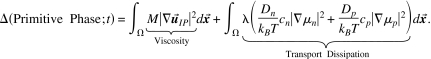28

Here $\nabla {\vec{\mathit{u}}}_{IP}$ is the strain rate tensor; M is the dynamic viscosity coefficient; and chemical potentials are written as Greek mu’s, μ_n=δE∕δc_n; μ_p=δE∕δc_p, see Eq. 19, following the nomenclature of physical chemistry.¹⁸⁶

DFT treatment of solid spheres.

Another way to handle the excluded volume of hard spheres is by including a term (for uncharged spheres) from DFT of liquids in the atomic scale energy. We use the uncharged terms from Refs. ^{58, 67, 68, 142, 187}. We simply replace the Lennard-Jones terms of Eqs. 24, 25, 26, 27 by the corresponding terms from Appendix C Perhaps someday an intermediate scale will produce correlations equivalent to those produced by the nonlocal integrals of DFT.

Theoretical model: Primitive model of ionic phase

Now we are in a position to write the primitive model of just the ionic fluid (without solvent water). This system will include the macroscopic (continuum) hydrodynamic variable ρ_IP, the mass density of the ionic phase (without solvent), velocity ${\vec{\mathit{u}}}_{IP}$ of the ionic phase (without solvent,) and hydrostatic pressure p_IP determined by the equation of state for ions (which without solvent form a compressible fluid) and is written as a function of time. On the atomic (microscopic scale) both the Lennard–Jones model [Eq. 25] and DFT model (Appendix C) have been implemented. Explicit formulas for ∇μ_n and ∇μ_p have been worked out for both, as described in Appendixes B. Explicit formulas for μ_n and μ_p are not possible because they are nonlocal, involving the electrical potential and finite volume effects throughout the global system.

Macroscopic conservation of mass is

$$\frac{\partial {\rho }_{IP}}{\partial t}+\nabla \cdot \left({\vec{\mathit{u}}}_{\text{IP}}{\rho }_{IP}\right)=0.$$ (29)

Macroscopic force balance (conservation of linear momentum) is

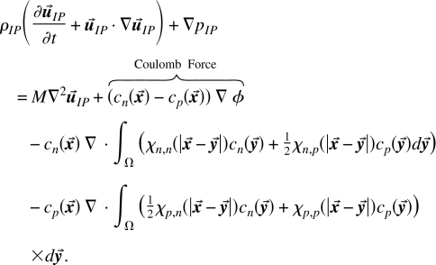(30)

In the above equation, the second term on the right hand side is the electric force which is the effect of charge on the macroscopic ionic phase (fluid). The second and third lines are the body forces due to the finite size effect. Notice that the concentration variables $c_n\left(\vec{\mathit{x}}\right)$ and $c_p\left(\vec{\mathit{x}}\right)$ in the body force terms cannot be moved inside the divergence. Their location implies that the divergence theorem (i.e., Green–Gauss formula) cannot put those concentration terms on the boundary. Thus these forces must be evaluated inside the bulk of the system and are given the name body force.

PNP for solid spheres.

Next we write time dependent PNP equations modified to include finite size effects,

$$\frac{\partial c_n}{\partial t}+\nabla \cdot \left(c_n{\vec{\mathit{u}}}_{IP}\right)=\nabla \cdot \left[D_n\left(\nabla c_n-\frac{e}{k_{B}T}{c}_n\nabla \varphi \right)\right]-\nabla \cdot \left[\frac{c_n\left(\vec{\mathit{x}}\right)}{k_{B}T}\left\{{\int }_{\Omega }\frac{12{\epsilon }_{n,n}{\left(a_n+a_n\right)}^{12}\left(\vec{\mathit{x}}-\vec{\mathit{y}}\right)}{{\left|\vec{\mathit{x}}-\vec{\mathit{y}}\right|}^{14}}{c}_n\left(\vec{\mathit{y}}\right)d\vec{\mathit{y}}+{\int }_{\Omega }\frac{6{\epsilon }_{n,p}{\left(a_n+a_p\right)}^{12}\left(\vec{\mathit{x}}-\vec{\mathit{y}}\right)}{{\left|\vec{\mathit{x}}-\vec{\mathit{y}}\right|}^{14}}{c}_p\left(\vec{\mathit{y}}\right)d\vec{\mathit{y}}\right\}\right],$$ (31)

$$\frac{\partial c_p}{\partial t}+\nabla \cdot \left(c_p{\vec{\mathit{u}}}_{IP}\right)=\nabla \cdot \left[D_p\left(\nabla c_p+\frac{e}{k_{B}T}{c}_p\nabla \varphi \right)\right]-\nabla \cdot \left[\frac{c_p\left(\vec{\mathit{x}}\right)}{k_{B}T}\left\{{\int }_{\Omega }\frac{12{\epsilon }_{p,p}{\left(a_p+a_p\right)}^{12}\left(\vec{\mathit{x}}-\vec{\mathit{y}}\right)}{{\left|\vec{\mathit{x}}-\vec{\mathit{y}}\right|}^{14}}{c}_p\left(\vec{\mathit{y}}\right)d\vec{\mathit{y}}+{\int }_{\Omega }\frac{6{\epsilon }_{n,p}{\left(a_n+a_p\right)}^{12}\left(\vec{\mathit{x}}-\vec{\mathit{y}}\right)}{{\left|\vec{\mathit{x}}-\vec{\mathit{y}}\right|}^{14}}{c}_n\left(\vec{\mathit{y}}\right)d\vec{\mathit{y}}\right\}\right].$$ (32)

The second terms on the left hand side of Eqs. 31, 32 represent the transport of the ions by a compressible fluid which is appropriate if the equations are applied only on the atomic scale. If we try to extend these equations to other scales, the proper form of the compressibility becomes an issue that needs to be resolved by experiment. These and the last two terms of Eq. 30 represent the balance of the internal forces (Newton’s third law).

It is important to verify Newton’s third law explicitly in problems of this sort. We deal with the water (solvent on the macroscopic scale), the ionic phase (fluid on the macroscopic scale), and the ionic particles (on an atomic scale). Newton’s third law has to be satisfied for each phase and all interactions among the phases.

Theoretical model: Solvent water

We turn now from the ionic phase to the solvent water. The solvent is treated traditionally as an incompressible fluid density ρ_f and velocity ${\vec{\mathit{u}}}_f$ (although treatment as a compressible fluid is possible if needed) using (generalized) energy and dissipation,

$$E\left(\mathbf{I}\mathbf{n}\mathbf{c}\mathbf{o}\mathbf{m}\mathbf{p}\mathbf{r}\mathbf{e}\mathbf{s}\mathbf{s}\mathbf{i}\mathbf{b}\mathbf{l}\mathbf{e}\mathbf{S}\mathbf{o}\mathbf{l}\mathbf{v}\mathbf{e}\mathbf{n}\mathbf{t}\right)={\int }_{\Omega }\frac{1}{2}{\rho }_f{\left|{\vec{\mathit{u}}}_f\right|}^{2}d\vec{\mathit{x}},$$ (33)

$$\Delta \left(\mathbf{I}\mathbf{n}\mathbf{c}\mathbf{o}\mathbf{m}\mathbf{p}\mathbf{r}\mathbf{e}\mathbf{s}\mathbf{s}\mathbf{i}\mathbf{b}\mathbf{l}\mathbf{e}\mathbf{S}\mathbf{o}\mathbf{l}\mathbf{v}\mathbf{e}\mathbf{n}\mathbf{t}\right)={\int }_{\Omega }{M}_f{\left|\nabla {\vec{\mathit{u}}}_f\right|}^{2}d\vec{\mathit{x}}.$$ (34)

Here, ∇⋅ρ_f=0 for an incompressible fluid. Applying the force balance law “Conservative Force=Dissipative Force” 7 to the equations for the incompressible solvent gives Navier–Stokes partial differential equations for an incompressible fluid with dynamic viscosity M_f,

$$\frac{\partial {\rho }_f}{\partial t}+{\vec{\mathit{u}}}_f\cdot \nabla {\rho }_f=0,$$ (35)

$$\nabla \cdot {\vec{\mathit{u}}}_f=0,$$ (36)

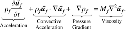(37)

Theoretical model: (Entire) Primitive solution

Finally, we can deal with the entire electrolyte, namely, the ionic solution consisting of the solvent and the primitive phase of ions by combining the (generalized) energy and the dissipation of the individual components using the simplest model for the interaction of the components. Later work may need to deal more carefully with the different scales of the components.

The (generalized) energy of the solution is simply the sum of the (generalized) energy of the components, namely, the sum of the energy of the ions in primitive phases (both atomic scale and macroscopic) and of the energy of the incompressible solvent Eq. 34. We do not write it out. We also will not bother to write “(generalized) energy” in every case from now on. It should be clear that “energy” in this paper is not just that defined in classical treatments of the first law of (equilibrium) thermodynamics.

The dissipation of the primitive solution is not just the sum of the dissipation of the components because the solvent can drag the ions and vice versa. Thus, the dissipation of the primitive solution is

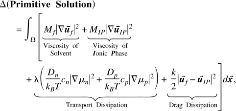(38)

where M_f is the dynamic viscosity, and ${\vec{\mathit{u}}}_f$ of the solvent fluid, M_IP, is the viscosity, and ${\vec{\mathit{u}}}_{IP}$ is the velocity of the Ionic Phase. The last term in Eq. 38 gives rise to an extra drag term $k\left({\vec{\mathit{u}}}_{IP}-{\vec{\mathit{u}}}_f\right)$ that will have to be added into Eq. 37 and also an extra term $-k\left({\vec{\mathit{u}}}_{IP}-{\vec{\mathit{u}}}_f\right)$ that will have to be added into Eq. 30. These two terms again reflect the balance of internal forces enforced by Newton’s third law. The frictional drag between solvent and ions is described to the lowest order approximation as a Stokes’ drag,

$$k=\gamma \rho \text{or}\gamma \left(c_n+c_p\right),\text{where}\text{the}\text{Stokes}\text{drag}\text{is}\gamma =6\pi M_f{a}_f,$$ (39)

where a_f is a generic description of the radius of the solvent particle. It is not clear a priori how much detail will be needed in describing the drag of the solvent on the ions and the ions on the solvent. This will be determined by solving the problem for specific cases of flow in mixed bulk solutions,^{34, 70, 90, 92, 93, 100, 101, 102, 103, 104, 105} or in ion channels, and seeing whether expressions for drag between water that arenotspecific for individual ions produce correlations similar to those observed experimentally^{188, 189} and traditionally attributed^{188, 190} to “single filing” (however, see Refs. ^{114, 129}). Perhaps, specific coefficients will need to be introduced into an EnVarA field theory of ionic solutions—as they have been in traditional theories of flux coupling in bulk and ion channels—to describe drag between one type of ion and other types of ions and water, with all the uncertainty that involves [e.g., how do the specific coefficients vary with concentration(s) in pure and mixed solutions?^{34, 90, 92, 100, 101, 102, 104}].

The total coupled system—involving solvent and macroscopic and atomic scale components of the entire solution—is given below. All the equations need to be solved together, in a simultaneous solution. Note the two physical sources of coupling between the solvent (water) and ion (primitive) phases. The drag term couples these phases dynamically, when there is relative movement. The phases are also coupled at equilibrium, when there is no motion, by Newton’s third law, and this coupling will produce at least some of the complexities normally dealt with “by hand” by the parameters of the equations of state.^{79, 80, 81, 162} The effect of the ions on the fluid is balanced by the effects of the fluid on the ions.

Complete ionic (primitive) solution.

Solvent water phase treated as incompressible.

$$\frac{\partial {\rho }_f}{\partial t}+{\vec{\mathit{u}}}_f\cdot \nabla {\rho }_f=0,$$ (40)

$$\nabla \cdot {\vec{\mathit{u}}}_f=0,$$ (41)

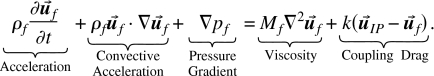(42)

Primitive ionic phases are macroscopic and atomic scale combined.

$$\frac{\partial {\rho }_{IP}}{\partial t}+\nabla \cdot \left({\vec{\mathit{u}}}_{IP}{\rho }_{IP}\right)=0,$$ (43)

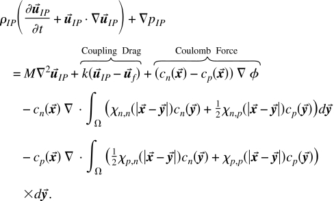(44)

Theoretical model: Generality of the energy variational approach

An energy variational treatment allows more generality and (possible) complexity than is usual in theories of ionic solution because (1) it includes all the bulk hydrodynamic behavior described by the Navier–Stokes equations; (2) it includes all the bulk hydrodynamic behavior of a compressible phase of ions; (3) it includes the atomic scale behavior of a PNP system including finite size ions that create their own electric field; (4) it allows boundary conditions that can drive flow, for example, when they are spatially nonuniform; and (5) it automatically computes interactions between all components and scales included in the models that describe dissipation and energy. In most models of ionic solutions,^{35, 80, 81, 84, 90, 92, 100, 101, 102, 162, 191} these interactions have to be put in by hand, sometimes with hundreds of parameters.⁷⁹

The generality of an energetic variational approach—which does not even distinguish between thermodynamic equilibrium and thermodynamic nonequilibrium—is a major potential advantage. For example, energy variational treatments will automatically reveal correlations in the flows of any of these components across all scales, even if pairwise interactions (like force laws of molecular dynamics) are not explicitly included in the energy function. The electrical potential is present on all scales and directly couples atomic and hydrodynamic bulk behavior in the resulting Euler–Lagrange field equations. The energy variational method also deals with double counting better than most [see discussion of double counting after Eq. 18]. It allows (in the future) combination of equations of state^{79, 80, 81, 88, 162} and (for example) our models of excluded volume—Lennard-Jones and density functional—each weighted with separate coupling constants, Lagrange multipliers, if we choose to handle them that way. One can choose coupling constants to fit data optimally using methods of inverse problems, if necessary to deal with issues of sensitivity and ill-posedness,^{106, 175} as we have in fitting PNP-DFT to properties of channels.⁵⁵

COMPUTATIONAL METHODS

Methods of numerical computations

Energetic variational methods produce integro-differential field equations that describe a wide range of systems under many conditions and thus with qualitatively different behaviors. Numerical procedures need to be tuned to the qualitative behavior of the system to be reasonably efficient. EnVarA requires numerical solutions of time dependent equations (because the real world is always time dependent). Steady state phenomena emerge as (hopefully stable) limits of time dependent phenomena, as they often do in the real world, so efficiency and stability are particularly important.

Computation of phenomena of molecular biology poses a stiff computational challenge. Biological phenomena are almost always slow (>10⁻⁴ s), but are usually controlled by a handful of key atoms in a few molecules, here channel proteins. Ion channels are nanovalves. Atomic structures of ion channels control macroscopic functions on macroscopic time scales. Displacements of 10⁻¹¹ m in the (time) averaged location of the key atoms of channel proteins have large effects on biological selectivity.^{15, 17, 63, 112, 192} The atoms move more or less at the speed of sound¹⁹³ and thus time scales from 10⁻¹⁶ to 10¹ s are directly involved in the behavior of ion channels.

We use finite element methods that reflect and take advantage of the underlying energetic variational structure of ion channel dynamics building on earlier work,^{30, 171, 194} particularly that of Ryham,^{167, 168} working with Liu that described the coupling of ions (PNP equations) and flow (Navier–Stokes equations) using a “mini” finite element to solve the (Navier)–Stokes dynamics. We use generalized mini elements to solve our model,¹⁹⁵ namely, the standard elements P_k−P_k−1, k=2,3,…. P_k are a set polynomials up to order k. We solve the drift-diffusion equation (Nernst–Planck) Eq. 20 with an efficient finite element method: edge averaged finite elements (EAFEs) that have been proposed¹⁹⁶ and studied extensively.^{167, 168} The method exploits the type of monotonicity of the operators in the equations. The Euler method is used to deal with time dependence. Ionic solutions are confined by insulating boundaries in experiments (and in channels). Insulating boundaries are described by no-flux boundary conditions derived by variational procedures. We use the following (pseudo) algorithm based on finite element discretization to solve the coupled Poisson–Nernst–Planck equations that include the effects of the finite volume of ions, for example, Eqs. 31, 32:

• Step 1. Set initial data $c_n^{\left(0\right)},c_p^{\left(0\right)},{\varphi }^{\left(0\right)}$ and k=1.

• Step 2. Set $c_n^{\left(k_{m-1}\right)}=c_n^{\left(k-1\right)}$, $c_p^{\left(k_{m-1}\right)}=c_p^{\left(k-1\right)}$, ${\varphi }_p^{\left(k_{m-1}\right)}={\varphi }_p^{\left(k-1\right)}$ for k=1,2,….

• Step 3. Solve the following finite dimensional equation for $c_n^{\left(k_m\right)},c_p^{\left(k_m\right)}$ with given $c_n^{\left(k_{m-1}\right)},c_p^{\left(k_{m-1}\right)},{\varphi }^{\left(k_{m-1}\right)}$ using EAFE:^{167, 168, 196}

  $$\frac{c_n^{\left(k_m\right)}-c_n^{\left(k_{m-1}\right)}}{dt}=\nabla \cdot D_n\left(\nabla c_n^{\left(k_m\right)}+\frac{z_{n}e}{k_{B}T}{c}_n^{\left(k_m\right)}\nabla {\varphi }^{\left(k_{m-1}\right)}+\nabla {\phi }_n\left(c_n^{\left(k_{m-1}\right)},c_p^{\left(k_{m-1}\right)}\right)\right),$$$$\frac{c_p^{\left(k_m\right)}-c_p^{\left(k_{m-1}\right)}}{dt}=\nabla \cdot D_p\left(\nabla c_p^{\left(k_m\right)}+\frac{z_{p}e}{k_{B}T}{c}_p^{\left(k_m\right)}\nabla {\varphi }^{\left(k_{m-1}\right)}+\nabla {\phi }_p\left(c_n^{\left(k_{m-1}\right)},c_p^{\left(k_{m-1}\right)}\right)\right),$$ 45

  where ${\phi }_j\left(c_n^{\left(k_{m-1}\right)},c_p^{\left(k_{m-1}\right)}\right),j=n,p$ are the chemical potential obtained from the finite volume energy and dt is the time step. The equation is written for monovalent anions n and cations p but programming was done for any ions of any charge.
• Step 4. Solve Poisson equation for given for ϕ^{(k_m−1∕2)} with given $c_n^{\left(k_m\right)},c_p^{\left(k_m\right)}$,

  $$\epsilon {\nabla }^2{\varphi }^{\left(k_{m-1∕2}\right)}=c_n^{\left(k_m\right)}-c_p^{\left(k_m\right)}.$$ (46)

  To prevent oscillatory behavior in this iteration we use a convex iteration scheme that has evolved^{167, 168, 196} from earlier work related to the Gummel iteration^{180, 197} of semiconductor physics,^{44, 198}

  $${\varphi }^{\left(k_m\right)}=c{\varphi }^{\left(k_{m-1∕2}\right)}+\left(1-c\right){\varphi }^{\left(k_{m-1}\right)},0<c\le 1.$$ (47)

• Step 5. Check self-consistency between $c_n^{\left(k_m\right)},c_p^{\left(k_m\right)},{\varphi }^{\left(k_m\right)}$. If consistent, then $c_n^{\left(k\right)}=c_n^{\left(k_m\right)},c_p^{\left(k\right)}=c_p^{\left(k_m\right)},{\varphi }^{\left(k\right)}={\varphi }^{\left(k_m\right)}$. Otherwise ϕ^(k_m−1)=ϕ^(k_m) and go to step 3.

• Step 6. Check the error between $c_n^{\left(k\right)},c_p^{\left(k\right)},{\varphi }^{\left(k\right)}$ and $c_n^{\left(k-1\right)},c_p^{\left(k-1\right)},{\varphi }^{\left(k-1\right)}$ with a criterion. If the error is less than a criterion, then print solution $c_n^{\left(k\right)},c_p^{\left(k\right)},{\varphi }^{\left(k\right)}$ and exit. Otherwise, set k=k+1 and go to step 2.

The numerical scheme for the PNP system has been verified by comparison to theoretical results, and in special cases to known solutions of the Poisson–Boltzmann and renormalized Poisson–Boltzmann equations. We verify by inspection that the numerical scheme has enough resolution to catch the boundary layer behaviors of the electrostatic potential.

RESULTS

We implement EnVarA here in a few special cases to show its feasibility. EnVarA yields a time dependent system of Euler–Lagrange equations, even if the properties of interest are stationary, developing after a long time. This is a blessing and a curse. It is a blessing because we learn much more of the system, and can understand or propose experiments in the time domain. It is a curse because the computations of time dependent phenomena produce complex phenomena not emphasized in classical experimental papers that often focus on simpler behavior seen in special steady state conditions.

Experiments are often designed to focus on particular parts of complex phenomena. The conditions that allow that focus often take many years to discover (consider, for example, sequence of papers needed to discover ionic conductance using the voltage clamp¹⁸⁴) and the preliminary survey experiments used to design that focus are often not reported in detail. After all, survey experiments give complex results that are usually quite confusing compared to focused experiments designed to illustrate key results.

Variational calculations report all the time dependent properties of the system; they correspond to the survey experiments. So we must survey ranges of parameters before we can focus on important experimental phenomena. The values of effective parameters needed to focus on particular parts of complex phenomena are not known ahead of time, and are hard to determine, particularly in simplified models computed in only one dimension. The numerical solutions of the time dependent Euler–Lagrange equations are slow, particularly since we are usually interested in the eventual steady state. Thus, our survey calculations are incomplete, and certainly have not yet isolated phenomena as clearly as experiments do (using protocols that often have taken decades to work out, we say in our defense).

Layering near a charged wall

We first calculate the property of “one dimensional spheres” near a highly charged wall in the presence of divalent and monovalent ions, e.g., hypothetical ions something like Ca²⁺ and Na⁺ Cl⁻. More precisely we use center to center interactions and evaluate the forces in one dimension in a long tradition starting with the statistical mechanics of uncharged spheres near walls.⁶⁵ We might be tempted to call these “rods” or one dimensional spheres, but the correct specification is the mathematics. We choose this system because it shows the ability of the variational method to deal with correlations in a highly charged, highly correlated system. Obviously, this idealization should be replaced by computations of spheres in three dimensions as soon as we can do those calculations. Indeed, we cannot quantitatively compare our results with MC simulations of real spheres¹³² until we work in three dimensions.

This reduced test case provides a wealth of complex behavior of great importance—judging from the hundreds of papers devoted to it—in a wide range of applications, from electrochemistry, to biophysics, to material science, where interactions of this type are important in determining the strength of cement¹⁹⁹ (i.e., calcium-silicate-hydrate). The literature of this field is well reviewed.^{132, 199, 200, 201} We have particularly used Ref. 200 for an overview of the entire field and Ref. 132 to show the wide variety of behaviors of such systems in MC simulations of the primitive model.

Figure 1 shows the spatial distribution of concentration (really, the number density in molar units) near a highly charged well comparable to those studied in the literature. The wall has charge density of 0.1 C∕m². Charge is shown divided by 1 C∕m³. The diameter of the ions is 0.1 nm and they have charges +2e and −1e, where e is the charge on a proton. Position is shown divided by nanometer. Dielectric coefficient was 78, temperature was 298 K, and the bulk concentration of ions was 1 M of the divalent cation and 2 M of the monovalent anion. The potential on the wall was set to −3.1 kT∕e, i.e., −80 mV in accord with MC simulations.²⁰² The dashed circles are shown for visual effect to show the size of the ions in the calculation. The densities change behavior when they reach the “excluded zone” produced by the finite diameter of the ions. Ions are not allowed to overlap with the wall.

Figure 1.

The number density (“concentration”) of ions near a charged wall. The wall has charge density of 0.1 C∕m². Charge is shown divided by 1 C∕m³. The diameter of the ions is 0.3 nm and they have charges of +2e and −1e, where e is the charge on a proton. Position is shown divided by nanometer. Dielectric coefficient was 78, temperature was 298 K, and the bulk concentration of ions was 1 M of the divalent cation and 2 M of the monovalent anion. The potential on the wall was set to −3.1 kT∕e, i.e., −80 mV in accord with MC simulations (Ref. ²⁰²). Energy coupling coefficients λ in EnVarA were 0.5. The dotted circles show the size of the ions in the calculation. Ions are not allowed to overlap with the wall and so the densities are smooth functions until they reach the excluded zone produced by finite diameter of the ions. Calculations were done using (solid lines) the PNP-DFT and PNP-LJ in the form described in the text and Appendixes A, C. The form of the DFT differs in detail (but not spirit) from that in recent literature (Refs. ⁶⁷, ⁶⁸, ²⁰³): we use DFT for uncharged interactions (following Refs. ⁶⁶, ¹⁴², ²⁰⁴) but we use EnVarA to deal with the electrostatics. EnVarA identically satisfies Gauss’ law (which is also one of the sum rules (Ref. ⁷² of statistical mechanics). This calculation is called PNP-DFT even though we report only equilibrium results: the variational method knows nothing of equilibrium and always computes a nonequilibrium transient response which may in special cases have no flows and a stationary solution. The results are qualitatively similar to the layering reported in MC simulations (Ref. ¹³²). Quantitative differences are expected because the systems are not identical. Most importantly, simulations were of hard spheres (whereas we use Lennard-Jones or DFT in one dimension). There are many other small differences; e.g., MC uses an approximation to the solution of Poisson’s equation (Ref. ²⁰⁵) that produces results independent of system size, but without definite error bounds (Refs. ¹³⁵, ²⁰⁶).

Dashed lines were computed with PNP+LJ (Lennard-Jones) and dashed lines with PNP-DFT as specified in the text and Appendixes A, C. Correlations are obviously involved at the high densities near the wall. This calculation is called PNP even though we report only equilibrium results that might be called (nonlinear) Poisson–Boltzmann: the variational method knows nothing of equilibrium and always computes a nonequilibrium transient response which may in special cases (like Fig. 1) have no flows and a stationary solution. Layering of this sort has been seen in previous calculations.^{65, 207, 208} It will not be clear whether a more precise treatment including an intermediate scale is necessary in Eqs. 24, 25, 26, 27 until we can do calculations in three dimensions.

Binding in channels

Calculations (Fig. 2) were also done of binding in a simple model of calcium channels that has proven quite successful.^{15, 17, 209} In this model, the active site of the calcium channel uses spheres with permanent charge to represent the side chains DEEA (aspartate glutamate glutamate alanine) that are known (from experiments¹⁴⁴) to mix with the ions and water in a structural motif very different from potassium channels. In our calculations, spheres are uniformly distributed at fixed locations within a cylindrical space of 3 Å long and 7 Å diameter (unlike MC simulations^{15, 17, 209} in which the spheres are free to move within that region) to reduce computation time. This and other details in the calculations (see above) mean that the variational method is not expected to give identical results to MC simulations. The ion diameters, geometry, and so on are otherwise as specified previously.^{15, 17, 209} Figure 2 shows the relative occupancy of the cylindrical space, that is to say, it shows the ratio of the spatial integral of the density of calcium to the spatial integral of the density of sodium, both within a cylindrical space of 3 Å long and 7 Å diameter. The densities are the stationary solution of the time dependent Euler–Lagrange equations. The concentration of sodium is maintained at 0.1 M on both sides of the channel. The concentration of calcium is varied and is shown on the horizontal axis.

Figure 2.

Binding of calcium to a DEEA channel. This figure shows the relative occupancy of the cylindrical space, that is to say, it shows the ratio of the spatial integral of the density of calcium (diameter of 1.98 Å) to the spatial integral of the density of sodium (diameter of 2.04 Å)—both within a cylindrical space of 3.5 Å radius and 3 Å length—of the stationary solution of the time dependent Euler–Lagrange equations. The concentration of sodium is maintained at 0.1 M on both sides of the channel. The concentration of calcium is varied and is shown on the horizontal axis. The dielectric constant was 80 and the temperature was 298 K. Geometrical setup is nearly the same as Figs. 1 and 2 of Ref. 15.

The binding computed is similar to that reported previously for the calcium channel.^{17, 112} Figure 3 shows similar calculations for the DEKA (aspartate glutamate lysine alanine) sodium channel. Here occupancy is reported, namely, the spatial integral of the density of either sodium or calcium which is the steady solutions of the Euler–Lagrange equations. The properties are similar to those reported previously¹⁵ with MC simulations of the sodium channel, where the physical and biological implications are extensively discussed.

Figure 3.

Binding of sodium to a DEKA channel. This figure shows the relative occupancy of the cylindrical space, that is to say, it shows the ratio of the spatial integral of the density of calcium to the spatial integral of the density of sodium, both within a cylindrical space of 3 Å long and 3.5 Å radius of the stationary solution of the time dependent Euler–Lagrange equations. The concentration of sodium is maintained at 0.1 M on both sides of the channel. The concentration of calcium is varied and is shown on the horizontal axis. The dielectric constant was 80 and the temperature was 298 K. Geometrical setup is nearly the same as Figs. 1 and 2 of Ref. 15.

Time dependent phenomena in ion channels

Figure 4 shows the time dependent current calculated after a step function is applied to a DEKA channel specified in Fig. 5 and the caption to Fig. 4. The current and time scales depend on a somewhat arbitrary assignment of effective parameters. The openings at the end of the channel are specified by flared cones as in Fig. 1 of Ref. 109 and subsequent papers so the one dimensional model is not dominated by artifactual electrical or diffusive resistance in the regions outside the channel. The time dependence seen in these records reflects changes of concentration of ions just outside the two ends of the channel. Such phenomena are not thought to be involved in the currents measured from squid sodium channels, but they are present in calcium channels²¹⁰ and potassium²¹¹ channels to cite only classical references.

Figure 4.

The time response to a step function of voltage of a DEKA sodium channel (Glu-Asp-Lys-Ala). The voltage pulse started at −0.09 V and switched to the indicated voltage at t=3 ms and then back to −0.09 at t=6 ms. As shown in Fig. 5, the channel is 20 Å long and has 7 Å diameter. The concentration of NaCl was 0.9 M on one side and 0.1 M on the other. The sodium ion had diameter of 2.04 Å and chloride ion had diameter of 3.62 Å, diffusion coefficients were 1.68 and 1.35 m²∕s, respectively. The dielectric constant was 80 and temperature was 298 K. No units are shown for current because the number of channels being computed is arbitrary.

Figure 5.

The setup for the calculations of time dependent current shown in Fig. 4. The blue line shows the boundary of the one dimensional channel. The steep spread between the lines is a one dimensional representation of the baths used because it reduces the “resistance” to current flow or flux. That is to say, the greater cross sectional area to flow allows more flow for a given gradient of electrochemical potential than in the narrow 7 Å (diameter) channel through the bilayer itself. The dashed line represents the lipid bilayer membrane. The distribution of fixed charge along the channel wall is labeled “configuration of side chains.” The concentration of salts is shown in the baths. The units of the axes are divided by angstroms.

Interpretation of current transients

The flow of current through real ion channels and the surrounding proteins and lipids is complex and involves many components. Those components had to be identified and separated before mechanisms could be identified, let alone studied. Indeed, the history of electrophysiology (before recordings were made on currents through single protein molecules²¹²) is in large measure the history of Cole²¹³ and Hodgkin’s¹⁸⁴ successful separation of components of current.

Separation was done in preparations of animal and plant cells put in situations designed to focus on and isolate particular components of current. The Anglo-American tradition was to choose preparations (e.g., the squid axon) and experimental methods (the voltage clamp) that isolated components. Workers in that tradition (importantly joined by German colleagues²¹²) depended on biology and experimental design as much as possible to isolate systems and tried to depend on theory and discussion as little as possible. The particular properties of the sodium channels of squid axon allow clear separation of components of currents. These properties ensure that accumulation of ions occurs on a longer time scale than the processes that open the channel (as viewed in macroscopic ensembles of channels). Most channels do not permit such separation, however. For example, in calcium channels,²¹⁰ opening processes and accumulation occur on the same time scale and are more or less inseparable. The channel opening process and accumulation occur on nearly the same scale as well, in squid potassium channels.^{211, 214} Indeed, it seems possible that the squid sodium channels are a special case, specialized to reduce change in concentration of ions during natural activity.²¹⁵ Accumulation of sodium ions would reduce inward current and limit the speed of conduction. Speed is what the squid giant axon (and squid itself) are all about from an evolutionary point of view.

Our calculations of the DEKA channel give results such as calcium and potassium channels. We do not know how to reproduce the special properties of squid sodium channels and conductance. In particular, our calculations show the pile-up of salt just outside the channel occurring much (say ten times) faster than in the squid.²¹¹ (By “salt” we mean neutral combinations of cation and anion, Na⁺ and Cl⁻, in Figs. 45.) Our calculations also often show rapid responses to steps in potential that describe the storage (“pile-up”) of charge inside the pore of the channel protein. These rapid pile-ups of charge occur on the same time scale as gating currents²¹⁶ found in real nerve cells²¹⁶ including the very fast component of gating current.²¹⁷ We do not show these rapid responses here because the calculations cannot easily be “corrected” for linear capacitance as are experimental measurements. Our calculated responses are not robust. Detailed comparisons with experiments must await calculations in three dimensions less dependent on assumed values of effective parameters. Thus, we do not know whether our buildup of charge might be a significant component of the gating current observed experimentally in sodium or calcium channels.

DISCUSSION

Ionic solutions have many diverse but specific properties arising from the interactions of their components on all scales and so it seems appropriate to treat them here as complex, not simple fluids. The diversity of properties of ionic solutions means that it is surely pretentious to write a general theory. A general theory must deal with all specific results, with the experiments and interpretations, theories, and simulations of many communities of scientists, painstakingly measured and (often) passionately debated over nearly a century. The authors can certainly not check a wide-ranging theory: we are not even physical chemists. The literature is vast beyond grasp and the many references cited here^{33, 34, 35, 36, 37, 38, 64, 68, 70, 81, 92, 99, 100, 102, 123, 137, 140, 142, 162, 204, 218, 219, 220} are not comprehensive, we fear they are not even an unbiased sample, despite our efforts. Our goal is to present enough detail in enough fields so other workers are motivated to adapt EnVarA to their specific needs and passions.

We propose a general variational analysis here because we suspect that correlations among ions are the key to understanding ionic solutions in bulk or ions in proteins.⁵² These correlations are the structure of ionic solutions. They change significantly with conditions. We believe that the structures cannot be assumed, and are difficult to model a priori with partial differential equations, because each charge is so correlated with so many other charges on both an atomic and global (macroscopic) scale. Simulations have difficulty computing such correlations because atomic motions must be computed on the 10⁻¹⁶ s time scale but biology occurs in macroscopic systems on macroscopic time scales and involves a biological mix of concentrations ranging from 10⁻¹¹–10¹m. These correlations arise naturally (and always self-consistently) in both physical solutions and in solutions of EnVarA. The pun on “solutions” is precise. In both the mathematics and physics, the electrical potential is present on all scales and directly couples atomic and hydrodynamic bulk behavior.

The structures of ionic solutions are self-organized⁵² (if we use biologists’ language) and form an induced fit of ion to ion, ionic atmosphere to ion, and ionic atmosphere and ions to a protein and its mobile side chains. The solutions of EnVarA are also self-organized. That is the great advantage of the variational procedure. Of course, the solutions of EnVarA only deal with phenomena and constraints that are present (or are implicit) in our model or energy equations. For example, the model of energy used here does not include complex behavior of solvent water. The model of a channel∕transporter here does not include proteins that do work on ions.^{118, 128}

Other kinds of mathematical analysis—for example, analysis of combined partial differential equations in idealized domains—are likely to (inadvertently) impose unnatural boundary conditions that constrain the charged particles in some way or the other and can only be maintained by unnatural artificially imposed flows of charge and energy. These unnatural flows produce unnatural correlations and structures in the mathematical solution that can severely distort the qualitative properties of the ionic system and so might be called “Dirichlet disasters” if one likes colorful language. For example, such a treatment of semiconductors as systems with constant (electric) fields would have impeded or prevented the discovery of transistors,²²¹ it seems safe to say.

Our variational approach to ionic solutions may fail because of errors in its formulation. We hope not. The theory may fail because it does not resolve some scales well enough. We expect so. Proteins have movements (“conformation changes”) over time scales from 10² to 10⁻¹³ s judging from the time scales of protein function, from classical measurements of dielectric dispersion,²²² and from molecular dynamics simulations. Our computations clearly cannot be expected to capture such a time range using a single time variable. We expect the theory to fail when it leaves something out altogether, particularly in biological applications, where proteins like enzymes²²³ or binding proteins²²⁴ do much more than provide a confining volume and electrostatic environment. In that case, EnVarA may help uncover (and then compute) the omitted pieces, correcting its own mistake.

Even in failure, however, we expect that EnVarA will be useful in studying ions in solutions and channels, as variational methods are in so many areas of physics, because EnVarA yields a field theory of a chemical system, thus including boundary conditions and flow without mathematical approximation. EnVarA yields specific working hypotheses—partial differential equations and boundary value problems with only a few adjustable parameters—that include all the interactions of the components of its energies. The equations can be tested against experiment in many applications, and then improved in a mathematically systematic and physically self-consistent way by adding or modifying components of the energy. EnVarA will enforce self-consistency. Experiments will enforce reality.

APPENDIX A: LENNARD-JONES TREATMENT OF FINITE SIZE

The repulsion potential is given by

$${\phi }_{R,i}=\frac{{\epsilon }_{i}a_i{}^{12}}{{\left|\vec{\mathit{x}}-\vec{\mathit{y}}\right|}^{12}},$$ (A1)

where a_i is the radius of ith ion, and ε_i is the energy constant (softness) of ion i. Then the repulsive energy E_i,j for ion i and j is defined by

$$E_{i,j}=\frac{1}{2}{\int }_{\Omega }{\int }_{\Omega }\frac{{\epsilon }_{i,j}{\left(a_i+a_j\right)}^{12}}{{\left|\vec{\mathit{x}}-\vec{\mathit{y}}\right|}^{12}}{c}_i\left(\vec{\mathit{x}}\right)c_j\left(\vec{\mathit{y}}\right)d\vec{\mathit{x}}d\vec{\mathit{y}}$$ (A2)

or

$$E=\frac{1}{2}{\int }_{\Omega }{\int }_{\Omega }\frac{{\epsilon }_{n,n}{\left(a_n+a_n\right)}^{12}}{{\left|\vec{\mathit{x}}-\vec{\mathit{y}}\right|}^{12}}{c}_n\left(\vec{\mathit{x}}\right)c_n\left(\vec{\mathit{y}}\right)d\vec{\mathit{x}}d\vec{\mathit{y}}+\frac{1}{2}{\int }_{\Omega }{\int }_{\Omega }\frac{{\epsilon }_{p,p}{\left(a_p+a_p\right)}^{12}}{{\left|\vec{\mathit{x}}-\vec{\mathit{y}}\right|}^{12}}{c}_p\left(\vec{\mathit{x}}\right)c_p\left(\vec{\mathit{y}}\right)d\vec{\mathit{x}}d\vec{\mathit{y}}+\frac{1}{2}{\int }_{\Omega }{\int }_{\Omega }\frac{{\epsilon }_{n,p}{\left(a_n+a_p\right)}^{12}}{{\left|\vec{\mathit{x}}-\vec{\mathit{y}}\right|}^{12}}{c}_n\left(\vec{\mathit{x}}\right)c_p\left(\vec{\mathit{y}}\right)d\vec{\mathit{x}}d\vec{\mathit{y}}.$$ (A3)

Here, we take a variational derivative with respect to the negative charge density c_n. Then we have following equation:

$$\delta E_{c_n}=\frac{1}{2}{\int }_{\Omega }{\int }_{\Omega }\frac{{\epsilon }_{n,n}{\left(a_n+a_n\right)}^{12}}{{\left|\vec{\mathit{x}}-\vec{\mathit{y}}\right|}^{12}}\delta c_n\left(\vec{\mathit{x}}\right)c_n\vec{\mathit{y}}d\vec{\mathit{x}}d\vec{\mathit{y}}+\frac{1}{2}{\int }_{\Omega }{\int }_{\Omega }\frac{{\epsilon }_{n,n}{\left(a_n+a_n\right)}^{12}}{{\left|\vec{\mathit{x}}-\vec{\mathit{y}}\right|}^{12}}{c}_n\left(\vec{\mathit{x}}\right)\delta c_n\vec{\mathit{y}}d\vec{\mathit{x}}d\vec{\mathit{y}}+\frac{1}{2}{\int }_{\Omega }{\int }_{\Omega }\frac{{\epsilon }_{n,p}{\left(a_n+a_p\right)}^{12}}{{\left|\vec{\mathit{x}}-\vec{\mathit{y}}\right|}^{12}}\delta c_n\left(\vec{\mathit{x}}\right)c_p\vec{\mathit{y}}d\vec{\mathit{x}}d\vec{\mathit{y}}={\int }_{\Omega }{\int }_{\Omega }\frac{{\epsilon }_{n,n}{\left(a_n+a_n\right)}^{12}}{{\left|\vec{\mathit{x}}-\vec{\mathit{y}}\right|}^{12}}\delta c_n\left(\vec{\mathit{x}}\right)c_n\vec{\mathit{y}}d\vec{\mathit{x}}d\vec{\mathit{y}}+\frac{1}{2}{\int }_{\Omega }{\int }_{\Omega }\frac{{\epsilon }_{n,p}{\left(a_n+a_p\right)}^{12}}{{\left|\vec{\mathit{x}}-\vec{\mathit{y}}\right|}^{12}}\delta c_n\left(\vec{\mathit{x}}\right)c_p\vec{\mathit{y}}d\vec{\mathit{x}}d\vec{\mathit{y}}.$$

Using the familiar identity

$$\delta c_n\left(\vec{\mathit{x}}\right)+\nabla \cdot \left(c_n\left(\vec{\mathit{x}}\right)\delta \vec{\mathit{x}}\right)=0,$$ (A4)

we take a variation with respect to $c_n\left(\vec{\mathit{x}}\right)$ and write it as a variation with respect to $\vec{\mathit{x}}$,

$$\delta E={\delta }_{\vec{\mathit{x}}}E={\int }_{\Omega }{\int }_{\Omega }{\nabla }_{\vec{\mathit{x}}}\frac{{\epsilon }_{n,n}{\left(a_n+a_n\right)}^{12}}{{\left|\vec{\mathit{x}}-\vec{\mathit{y}}\right|}^{12}}{c}_n\left(\vec{\mathit{x}}\right)\delta \vec{\mathit{x}}{c}_n\left(\vec{\mathit{y}}\right)d\vec{\mathit{x}}d\vec{\mathit{y}}+\frac{1}{2}{\int }_{\Omega }{\int }_{\Omega }{\nabla }_{\vec{\mathit{x}}}\frac{{\epsilon }_{n,p}{\left(a_n+a_p\right)}^{12}}{{\left|\vec{\mathit{x}}-\vec{\mathit{y}}\right|}^{12}}{c}_p\left(\vec{\mathit{x}}\right)\delta \vec{\mathit{x}}{c}_n\left(\vec{\mathit{y}}\right)d\vec{\mathit{x}}d\vec{\mathit{y}}=-{\int }_{\Omega }{\int }_{\Omega }\frac{12{\epsilon }_{n,n}{\left(a_n+a_n\right)}^{12}\left(\vec{\mathit{x}}-\vec{\mathit{y}}\right)}{{\left|\vec{\mathit{x}}-\vec{\mathit{y}}\right|}^{14}}{c}_n\left(\vec{\mathit{x}}\right)c_n\left(\vec{\mathit{y}}\right)\delta \vec{\mathit{x}}d\vec{\mathit{x}}d\vec{\mathit{y}}-{\int }_{\Omega }{\int }_{\Omega }\frac{6{\epsilon }_{n,p}{\left(a_n+a_p\right)}^{12}\left(\vec{\mathit{x}}-\vec{\mathit{y}}\right)}{{\left|\vec{\mathit{x}}-\vec{\mathit{y}}\right|}^{14}}{c}_n\left(\vec{\mathit{x}}\right)c_p\left(\vec{\mathit{y}}\right)\delta \vec{\mathit{y}}d\vec{\mathit{x}}d\vec{\mathit{y}}.$$ (A5)

Also, for variation on $\vec{\mathit{x}}$ in terms of $c_p\left(\vec{\mathit{x}}\right)$,

$$\delta \left(c_p\vec{\mathit{x}}\right)+\nabla \cdot \left(c_p\left(\vec{\mathit{x}}\right)\delta \vec{\mathit{x}}\right)=0,$$ (A6)

$$\delta E={\delta }_{\vec{\mathit{x}}}E=-{\int }_{\Omega }{\int }_{\Omega }\frac{12{\epsilon }_{p,p}{\left(a_p+a_p\right)}^{12}\left(\vec{\mathit{x}}-\vec{\mathit{y}}\right)}{{\left|\vec{\mathit{x}}-\vec{\mathit{y}}\right|}^{14}}{c}_p\left(\vec{\mathit{x}}\right)c_p\left(\vec{\mathit{y}}\right)\delta \vec{\mathit{x}}d\vec{\mathit{x}}d\vec{\mathit{y}}-{\int }_{\Omega }{\int }_{\Omega }\frac{6{\epsilon }_{n,p}{\left(a_n+a_p\right)}^{12}\left(\vec{\mathit{x}}-\vec{\mathit{y}}\right)}{{\left|\vec{\mathit{x}}-\vec{\mathit{y}}\right|}^{14}}{c}_p\left(\vec{\mathit{x}}\right)c_n\left(\vec{\mathit{y}}\right)\delta \vec{\mathit{x}}d\vec{\mathit{x}}d\vec{\mathit{y}}.$$ (A7)

Attractive (or other) forces can be included either as another component of the energy in the atomic scale energy Eq. 18 and atomic scale dissipation 28 or by including a traditional description of the excess free energy of ionic solutions³⁵, ³⁶, ³⁷, ³⁸, ⁹⁰ into the macroscopic scale equations of the compressible ionic fluid, e.g., using the functionals of the DFT of liquids.⁴⁵, ⁵⁸, ¹³⁷, ¹⁴⁰, ¹⁴¹, ¹⁴², ²⁰⁸, ²¹⁹, ²²⁰ An attractive Lennard-Jones force could be easily added since it has the same form as the repulsive term used above Eq. A1. Other models of interatomic forces could be used, including (for example) estimates of the “potential of mean force” between ions (or molecules) determined from the radial distribution functions in simulations or experiments.²²⁰ Adding an attractive term of any type will yield a different partial differential equation from Eqs. 31, 32.

APPENDIX B: THE ELECTROCHEMICAL FORCES ∇μ_n AND ∇μ_p INCLUDING THE EFFECTS OF FINITE SIZE IONS

In Appendix A we derived just the part of the electrochemical forces ∇μ_n and ∇μ_p related to the finite size of ions. Here, we complete the system. We compute the diffusional and electrostatic terms of the electrochemical forces,

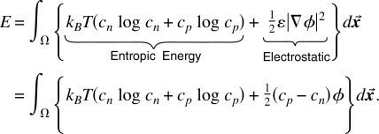(B1)

Since ϕ is the solution of Poisson equation, we have that

$$\varphi \left(\vec{\mathit{x}}\right)={\int }_{\Omega }\frac{G\left(\vec{\mathit{x}},\vec{\mathit{y}}\right)}{\epsilon }\left(c_n\left(\vec{\mathit{y}}\right)-c_p\left(\vec{\mathit{y}}\right)\right)d\vec{\mathit{y}}$$ (B2)

with Green’s kernel $G\left(\vec{x},\vec{y}\right)$. Substituting Eq. B2 with ϕ, the generalized energy E of Eq. B1 becomes

$$E={\int }_{\Omega }\left\{k_{B}T\left(c_n\left(\vec{\mathit{x}}\right)\text{log}{c}_n\left(\vec{\mathit{x}}\right)+c_p\left(\vec{\mathit{x}}\right)\text{log}{c}_p\left(\vec{\mathit{x}}\right)\right)+\left(c_p\left(\vec{\mathit{x}}\right)-c_n\left(\vec{\mathit{x}}\right)\right){\int }_{\Omega }\frac{G\left(\vec{\mathit{x}},\vec{\mathit{y}}\right)}{\epsilon }\left(c_n\left(\vec{\mathit{y}}\right)-c_p\left(\vec{\mathit{y}}\right)\right)d\vec{\mathit{y}}\right\}d\vec{\mathit{x}}.$$ (B3)

Hence, the variational derivative employing Eq. A4 leads us to

$$\delta E_{c_n}={\int }_{\Omega }\left\{\delta c_n\left(\vec{\mathit{x}}\right)k_{B}T\left(\text{log}{c}_n\left(\vec{\mathit{x}}\right)+1\right)-\frac{\delta c_n\left(\vec{\mathit{x}}\right)}{2}\int \frac{G\left(\vec{\mathit{x}},\vec{\mathit{y}}\right)}{\epsilon }\left(c_n\left(\vec{\mathit{y}}\right)-c_p\left(\vec{\mathit{y}}\right)\right)d\vec{\mathit{y}}\right\}d\vec{\mathit{x}}+{\int }_{\Omega }\left\{\frac{\left(c_p\left(\vec{\mathit{x}}\right)-c_n\left(\vec{\mathit{x}}\right)\right)}{2}\int \frac{G\left(\vec{\mathit{x}},\vec{\mathit{y}}\right)}{\epsilon }\delta c_n\left(\vec{\mathit{y}}\right)d\vec{\mathit{y}}\right\}d\vec{\mathit{x}},$$ (B4)

$$={\int }_{\Omega }\left\{\delta c_n\left(\vec{\mathit{x}}\right)\left(k_{B}T\left(\text{log}{c}_n\left(\vec{\mathit{x}}\right)+1\right)-{\int }_{\Omega }\frac{G\left(\vec{\mathit{x}},\vec{\mathit{y}}\right)}{2\epsilon }\left(c_n\left(\vec{\mathit{y}}\right)-c_p\left(\vec{\mathit{y}}\right)\right)d\vec{\mathit{y}}\right)\right\}d\vec{\mathit{x}}-{\int }_{\Omega }\left\{\left(c_n\left(\vec{\mathit{y}}\right)-c_p\left(\vec{\mathit{y}}\right)\right){\int }_{\Omega }\frac{G\left(\vec{\mathit{y}},\vec{\mathit{x}}\right)}{2\epsilon }\delta c_n\left(\vec{\mathit{x}}\right)d\vec{\mathit{x}}\right\}d\vec{\mathit{y}},$$ (B5)

$$={\int }_{\Omega }\left\{\delta c_n\left(\vec{\mathit{x}}\right)\left(k_{B}T\left(\text{log}{c}_n\left(\vec{\mathit{x}}\right)+1\right)-{\int }_{\Omega }\frac{G\left(\vec{\mathit{x}},\vec{\mathit{y}}\right)}{\epsilon }\left(c_n\left(\vec{\mathit{y}}\right)-c_p\left(\vec{\mathit{y}}\right)\right)d\vec{\mathit{y}}\right)\right\}d\vec{\mathit{x}}=-{\int }_{\Omega }\nabla \cdot \left(c_n\left(\vec{\mathit{x}}\right)\delta \vec{\mathit{x}}\right)\left\{k_{B}T\left(\text{log}{c}_n\left(\vec{\mathit{x}}\right)+1\right)-\varphi \left(\vec{\mathit{x}}\right)\right\}d\vec{\mathit{x}}={\int }_{\Omega }\left\{c_n\left(\vec{\mathit{x}}\right)\nabla \left(k_{B}T\left(\text{log}{c}_n\left(\vec{\mathit{x}}\right)+1\right)-\varphi \left(\vec{\mathit{x}}\right)\right)\right\}\delta \vec{\mathit{x}}d\vec{\mathit{x}}.$$ (B6)

Similarly, for the variational derivative with respect to $c_p\left(\vec{\mathit{x}}\right)$,

$$\delta E_{c_p}={\int }_{\Omega }\left\{\delta c_p\left(\vec{\mathit{x}}\right)k_{B}T\left(\text{log}{c}_p\left(\vec{\mathit{x}}\right)+1\right)-\frac{\delta c_p\left(\vec{\mathit{x}}\right)}{2}{\int }_{\Omega }\frac{G\left(\vec{\mathit{x}},\vec{\mathit{y}}\right)}{\epsilon }\left(c_n\left(\vec{\mathit{y}}\right)-c_p\left(\vec{\mathit{y}}\right)\right)d\vec{\mathit{y}}\right\}d\vec{\mathit{x}}+{\int }_{\Omega }\left\{\frac{\left(c_p\left(\vec{\mathit{x}}\right)-c_n\left(\vec{\mathit{x}}\right)\right)}{2}{\int }_{\Omega }\frac{G\left(\vec{\mathit{x}},\vec{\mathit{y}}\right)}{\epsilon }\delta c_p\left(\vec{\mathit{y}}\right)d\vec{\mathit{y}}\right\}d\vec{\mathit{x}}={\int }_{\Omega }\left\{c_p\left(\vec{\mathit{x}}\right)\nabla \left(k_{B}T\left(\text{log}{c}_p\left(\vec{\mathit{x}}\right)+1\right)+\varphi \left(\vec{\mathit{x}}\right)\right)\right\}\delta \vec{\mathit{x}}d\vec{\mathit{x}}.$$ (B7)

The results of Appendixes B, C give explicit expressions for the electrochemical forces ∇μ_n and ∇μ_p.

APPENDIX C: HARD SPHERE ENERGY IN DENSITY FUNCTIONAL THEORY

The (generalized) energy of six types of hard spheres (Na⁺, K⁺, Ca²⁺, Cl⁻, and X⁻) solid uncharged spheres is described in DFT (Refs. ⁵⁸, ⁶⁷, ⁶⁸, ¹⁴², ¹⁸⁷) by the following equations:

$$E\left(\text{Hard}\text{Sphere}\right)=E_{\text{HS}}^{\text{DFT}}=\int {\Phi }_{\text{HS}}\left(\left\{n_{\alpha }\left(\vec{\mathit{y}}\right)\right\},\left\{{\vec{\mathit{n}}}_{\beta }\left(\vec{\mathit{y}}\right)\right\}\right)d\vec{\mathit{y}},$$ (C1)

where

$${\Phi }_{\text{HS}}\left(\left\{n_{\alpha }\left(\vec{\mathit{y}}\right)\right\},\left\{{\vec{\mathit{n}}}_{\beta }\left(\vec{\mathit{y}}\right)\right\}\right)=-n_0\text{\hspace{0.17em}log}\left(1-n_3\right)+\frac{n_1{n}_2-{\vec{\mathit{n}}}_4\cdot {\vec{\mathit{n}}}_5}{1-n_3}+\frac{n_2^3}{24\pi {\left(1-n_3\right)}^2}{\left(1-\frac{{\vec{\mathit{n}}}_5\cdot {\vec{\mathit{n}}}_5}{n_2^2}\right)}^3,$$ (C2)

and

$$\begin{array}{ll}\text{for}\alpha =0,1,2,3\hfill & n_{\alpha }\left(\vec{\mathit{x}}\right)=\sum _i\int c_i\left(\vec{\mathit{y}}\right){\omega }_i^{\left(\alpha \right)}\left(\vec{\mathit{y}}-\vec{\mathit{x}}\right)d\vec{\mathit{y}},\hfill \\ \text{for}\beta =4,5\hfill & {\vec{n}}_{\beta }\left(\vec{\mathit{x}}\right)=\sum _i\int c_i\left(\vec{\mathit{y}}\right){\vec{\mathbf{\omega }}}_i^{\left(\beta \right)}\left(\vec{\mathit{y}}-\vec{\mathit{x}}\right)d\vec{\mathit{y}},\hfill \end{array}$$ (C3)

$$4\pi a_i^2{\omega }_i^{\left(0\right)}\left(\vec{\mathit{r}}\right)=4\pi a_i{\omega }_i^{\left(1\right)}\left(\vec{\mathit{r}}\right)={\omega }_i^{\left(2\right)}\left(\vec{\mathit{r}}\right),$$$$4\pi a_i{\vec{\mathbf{\omega }}}_i^{\left(4\right)}\left(\vec{\mathit{r}}\right)={\vec{\mathbf{\omega }}}_i^{\left(5\right)}\left(\vec{\mathit{r}}\right),$$$${\omega }_i^{\left(2\right)}\left(\vec{\mathit{r}}\right)=\delta \left(\left|\vec{\mathit{r}}\right|-a_i\right),$$$${\omega }_i^{\left(3\right)}\left(\vec{\mathit{r}}\right)=\theta \left(\left|\vec{\mathit{r}}\right|-a_i\right),$$$${\vec{\mathbf{\omega }}}_i^{\left(5\right)}\left(\vec{\mathit{r}}\right)=\frac{\vec{\mathit{r}}}{\left|\vec{\mathit{r}}\right|}\delta \left(\left|\vec{\mathit{r}}\right|-a_i\right),$$ C4

where ${\Phi }_{\text{HS}}\left(\left\{n_{\alpha }\right\},\left\{{\vec{\mathit{n}}}_{\beta }\right\}\right)$ is the excess free energy density that depends on the “nonlocal” densities $\left\{n_{\alpha }\right\},\left\{{\vec{\mathit{n}}}_{\beta }\right\}$; a_i is the radius of ion species i; $\delta \left(\vec{\mathit{x}}\right)$ is the Dirac delta function; and $\theta \left(\vec{\mathit{x}}\right)$ is the unit step function,

$$\theta \left(\vec{\mathit{x}}\right)=\{\begin{array}{cc}0,& \vec{\mathit{x}}>0\\ 1,& \vec{\mathit{x}}\le 0.\end{array}\phantom{\}}$$ (C5)

The chemical potential is given for α=0,…,3,β=4,5,

$${\mu }_i^{\text{HS}}\left(\vec{\mathit{x}}\right)=k_{B}T\left(\sum _{\alpha }\int \frac{\partial {\Phi }_{\text{HS}}}{\partial n_{\alpha }}\left(\vec{\mathit{y}}\right){\omega }_i^{\left(\alpha \right)}\left(\vec{\mathit{x}}-\vec{\mathit{y}}\right)d\vec{\mathit{y}}+\sum _{\beta }\int \frac{\partial {\Phi }_{\text{HS}}}{\partial {\vec{\mathit{n}}}_{\beta }}\left(\vec{\mathit{y}}\right){\vec{\mathbf{\omega }}}_i^{\left(\beta \right)}\left(\vec{\mathit{x}}-\vec{\mathit{y}}\right)d\vec{\mathit{y}}\right).$$ (C6)

The force term in the right hand side of the momentum equation is derived as

$${\text{force}}_i^{\text{HS}\text{to}\text{Fluids}}\left(\vec{\mathit{x}}\right)=-c_i\left(\vec{\mathit{x}}\right)\nabla {\mu }_i^{\text{HS}}\left(\vec{\mathit{x}}\right).$$ (C7)

References

- Yue P., Feng J. J., Liu C., and Shen J., J. Fluid Mech. 515, 293 (2004). 10.1017/S0022112004000370 [DOI] [Google Scholar]
- Lin F. -H., Liu C., and Zhang P., Commun. Pure Appl. Math. 58, 1437 (2005). 10.1002/cpa.20074 [DOI] [Google Scholar]
- Doi M. and Edwards S. F., The Theory of Polymer Dynamics (Oxford University Press, New York, 1988). [Google Scholar]
- Eringen A. C., Nonlocal Continuum Theories (Springer, New York, 2002). [Google Scholar]
- Liu C., in Multi-Scale Phenomena in Complex Fluids: Modeling, Analysis and Numerical Simulation, Series in Contemporary Applied Math, Vol. 12, edited by Hou T. Y., Liu C., and Liu J.-G. (World Scientific Publishing, Singapore, 2008). [Google Scholar]
- Bird R. B., Armstrong R. C., and Hassager O., Dynamics of Polymeric Fluids, Fluid Mechanics (Wiley, New York, 1977) [Google Scholar]; Bird R. B., Hassager O., Armstrong R. C., and Curtiss C. F., Dynamics of Polymeric Fluids, Kinetic Theory (Wiley, New York, 1977). [Google Scholar]
- Yue P., Feng J. J., Liu C., and Shen J., J. Fluid Mech. 540, 427 (2005). 10.1017/S0022112005006166 [DOI] [Google Scholar]
- Sheng P., Zhang J., and Liu C., Prog. Theor. Phys. Suppl. 175, 131 (2008). 10.1143/PTPS.175.131 [DOI] [Google Scholar]
- Zhang J., Gong X., Liu C., Wen W., and Sheng P., Phys. Rev. Lett. 101, 194503 (2008). 10.1103/PhysRevLett.101.194503 [DOI] [PubMed] [Google Scholar]
- Ryham R., Liu C., and Zikatanov L., Discrete Contin. Dyn. Syst., Ser. B 8, 649 (2007). [Google Scholar]
- Franklin B., Brownrigg W., and Farish M., Philos. Trans. R. Soc. London 64, 445 (1774) 10.1098/rstl.1774.0044 [DOI] [Google Scholar]; Velarde M. G., Interfacial Phenomena and the Marangoni Effect (Springer, New York, 2003). [Google Scholar]
- Goulding D., Hansen J. P., and Melchionna S., Phys. Rev. Lett. 85, 1132 (2000). 10.1103/PhysRevLett.85.1132 [DOI] [PubMed] [Google Scholar]
- Goulding D., Melchionna S., and Hansen J. -P., Phys. Chem. Chem. Phys. 3, 1644 (2001). 10.1039/b009434j [DOI] [Google Scholar]
- Eisenberg B., Biophys. Chem. 100, 507 (2003). 10.1016/S0301-4622(02)00302-2 [DOI] [PubMed] [Google Scholar]
- Boda D., Nonner W., Valisko M., Henderson D., Eisenberg B., and Gillespie D., Biophys. J. 93, 1960 (2007). 10.1529/biophysj.107.105478 [DOI] [PMC free article] [PubMed] [Google Scholar]
- Boda D., Valisko M., Eisenberg B., Nonner W., Henderson D., and Gillespie D., Phys. Rev. Lett. 98, 168102 (2007). 10.1103/PhysRevLett.98.168102 [DOI] [PubMed] [Google Scholar]
- Boda D., Valisko M., Henderson D., Eisenberg B., Gillespie D., and Nonner W., J. Gen. Physiol. 133, 497 (2009). 10.1085/jgp.200910211 [DOI] [PMC free article] [PubMed] [Google Scholar]
- Boda D., Busath D. D., Henderson D., and Sokolowski S., J. Phys. Chem. B 104, 8903 (2000). 10.1021/jp0019658 [DOI] [Google Scholar]
- Nonner W., Catacuzzeno L., and Eisenberg B., Biophys. J. 79, 1976 (2000). 10.1016/S0006-3495(00)76446-0 [DOI] [PMC free article] [PubMed] [Google Scholar]
- Goldstein H., Classical Mechanics, 2nd ed. (Addison-Wesley, Reading, MA, 1980). [Google Scholar]
- Biot M. A., Variational Principles in Heat Transfer: A Unified Lagrangian Analysis of Dissipative Phenomena (Oxford University Press, New York, 1970). [Google Scholar]
- Gelfand I. M. and Fromin S. V., Calculus of Variations (Dover, New York, 1963). [Google Scholar]
- Arnold A., Carrillo J. A., Desvillettes L., Dolbeault J., Jüngel A., Lederman C., Markowich P. A., Toscani G., and Villani C., Monatsh. Math. 142, 35 (2004). 10.1007/s00605-004-0239-2 [DOI] [Google Scholar]
- Rayleigh L., previously Strutt J. W., Proc. London Math. Soc. IV, 357 (1873). [Google Scholar]
- Onsager L., Phys. Rev. 37, 405 (1931). 10.1103/PhysRev.37.405 [DOI] [Google Scholar]
- Onsager L., Phys. Rev. 38, 2265 (1931). 10.1103/PhysRev.38.2265 [DOI] [Google Scholar]
- Arnold V. I., Mathematical Methods of Classical Mechanics, 2nd ed. (Springer, New York, 1997). [Google Scholar]
- Taylor J., Classical Mechanics (University Science Books, Sausalito, CA, 2005). [Google Scholar]
- Landau L. D. and Lifshitz E. M., Statistical Physics, Course of Theoretical Physics Vol. 5, 3rd ed. (Butterworths, London, 1996). [Google Scholar]
- Du Q., Hyon Y., and Liu C., Multiscale Model. Simul. 7, 978 (2008). 10.1137/070708287 [DOI] [Google Scholar]
- Du Q., Liu C., and Yu P., Multiscale Modeling & Simulation 4, 709 (2005). 10.1137/040612038 [DOI] [Google Scholar]
- Yu P., Du Q., and Liu C., Multiscale Model. Simul. 3, 895 (2005). 10.1137/030602794 [DOI] [Google Scholar]
- Lee L. L., Molecular Thermodynamics of Nonideal Fluids (Butterworth-Heinemann, New York, 1988). [Google Scholar]
- Pitzer K. S., Thermodynamics, 3rd ed. (McGraw-Hill, New York, 1995). [Google Scholar]
- Barthel J., Krienke H., and Kunz W., Physical Chemistry of Electrolyte Solutions: Modern Aspects (Springer, New York, 1998). [Google Scholar]
- Durand-Vidal S., Simonin J. -P., and Turq P., Electrolytes at Interfaces (Kluwer, Boston, 2000). [Google Scholar]
- Fawcett W. R., Liquids, Solutions, and Interfaces: From Classical Macroscopic Descriptions to Modern Microscopic Details (Oxford University Press, New York, 2004). [Google Scholar]
- Lee L. L., Molecular Thermodynamics of Electrolyte Solutions (World Scientific Singapore, 2008). [Google Scholar]
- Warshel A. and Russell S. T., Q. Rev. Biophys. 17, 283 (1984). 10.1017/S0033583500005333 [DOI] [PubMed] [Google Scholar]
- Gilson M. K. and Honig B., Biopolymers 25, 2097 (2004) 10.1002/bip.360251106 [DOI] [PubMed] [Google Scholar]; Roux B., in Computational Biophysics, edited by Becker O., MacKerrel A. D., Roux B., and Watanabe M. (Marcel Dekker, New York, 2001), Chap. 7, pp. 133–155 [Google Scholar]; Nielsen J. E. and McCammon J. A., Protein Sci. 12, 1894 (2003) 10.1110/ps.03114903 [DOI] [PMC free article] [PubMed] [Google Scholar]; Dzubiella J., Swanson J. M., and McCammon J. A., Phys. Rev. Lett. 96, 087802 (2006). 10.1103/PhysRevLett.96.087802 [DOI] [PubMed] [Google Scholar]
- Davis M. E. and McCammon J. A., Chem. Rev. (Washington, D.C.) 90, 509 (1990) 10.1021/cr00101a005 [DOI] [Google Scholar]; Antosiewicz J., McCammon J. A., and Gilson M. K., Biochemistry 35, 7819 (1996). 10.1021/bi9601565 [DOI] [PubMed] [Google Scholar]
- Van Roosbroeck W., Bell Syst. Tech. J. 29, 560 (1950). [Google Scholar]
- Selberherr S., Analysis and Simulation of Semiconductor Devices (Springer-Verlag, New York, 1984). [Google Scholar]
- Jerome J. W., Analysis of Charge Transport. Mathematical Theory and Approximation of Semiconductor Models (Springer-Verlag, New York, 1995). [Google Scholar]
- Eisenberg R. and Chen D., Biophys. J. 64, A22 (1993). [DOI] [PMC free article] [PubMed] [Google Scholar]
- Eisenberg R. S., J. Membr. Biol. 150, 1 (1996). 10.1007/s002329900026 [DOI] [PubMed] [Google Scholar]
- Eisenberg R. S., in New Developments and Theoretical Studies of Proteins, edited by Elber R. (World Scientific, Philadelphia, 1996), Vol. 7, p. 269. [Google Scholar]
- Bazant M. Z., Thornton K., and Ajdari A., Phys. Rev. E 70, 021506 (2004). 10.1103/PhysRevE.70.021506 [DOI] [PubMed] [Google Scholar]
- Roth R. and Gillespie D., Phys. Rev. Lett. 95, 247801 (2005). 10.1103/PhysRevLett.95.247801 [DOI] [PubMed] [Google Scholar]
- Miedema H., Vrouenraets M., Wierenga J., Eisenberg B., Gillespie D., Meijberg W., and Nonner W., Biophys. J. 91, 4392 (2006). 10.1529/biophysj.106.087114 [DOI] [PMC free article] [PubMed] [Google Scholar]
- Gillespie D., Biophys. J. 94, 1169 (2008). 10.1529/biophysj.107.116798 [DOI] [PMC free article] [PubMed] [Google Scholar]
- Bardhan J. P., Eisenberg R. S., and Gillespie D., Phys. Rev. E 80, 011906 (2009). 10.1103/PhysRevE.80.011906 [DOI] [PMC free article] [PubMed] [Google Scholar]
- Lundstrom M., Fundamentals of Carrier Transport, 2nd ed. (Addison-Wesley, New York, 2000). 10.1017/CBO9780511618611 [DOI] [Google Scholar]
- Boyd T. J. M. and Sanderson J. J., The Physics of Plasmas (Cambridge University Press, New York, 2003) 10.1017/CBO9780511755750 [DOI] [Google Scholar]; Goldston R. J. and Rutherford P. H., Introduction to Plasma Physics (Institute of Physics, London, 1995) [Google Scholar]; Birdsall C. K. and Langdon A. B., Plasma Physics via Computer Simulation (Institute of Physics, London, 1991). 10.1887/0750301171 [DOI] [Google Scholar]
- Burger M., Eisenberg R. S., and Engl H., SIAM J. Appl. Math. 67, 960 (2007). 10.1137/060664689 [DOI] [Google Scholar]
- Eisenberg B., Phys. Today 59(4), 12 (2006). [Google Scholar]
- van der Straaten T. A., Tang J., Eisenberg R. S., Ravaioli U., and Aluru N. R., J. Comput. Electron. 1, 335 (2002) 10.1023/A:1020787222235 [DOI] [Google Scholar]; Hollerbach U., Chen D. P., Busath D. D., and Eisenberg B., Langmuir 16, 5509 (2000) 10.1021/la991525b [DOI] [Google Scholar]; Eisenberg B., “Permeation as a diffusion process,” http://www.biophysics.org/btol/channel.html#5, 2000; Hollerbach U., Chen D., Nonner W., and Eisenberg B., Biophys. J. 76, A205 (1999) [Google Scholar]; Chen D., Eisenberg R., Jerome J., and Shu C., Biophys. J. 69, 2304 (1995) 10.1016/S0006-3495(95)80101-3 [DOI] [PMC free article] [PubMed] [Google Scholar]; Barcilon V., Chen D. P., and Eisenberg R. S., SIAM J. Appl. Math. 52, 1405 (1992) 10.1137/0152081 [DOI] [Google Scholar]; Graf P., Nitzan A., Kurnikova M. G., and Coalson R. D., J. Phys. Chem. B 104, 12324 (2000) 10.1021/jp001282s [DOI] [Google Scholar]; Cardenas A. E., Coalson R. D., and Kurnikova M. G., Biophys. J. 79, 80 (2000) 10.1016/S0006-3495(00)76275-8 [DOI] [PMC free article] [PubMed] [Google Scholar]; Kurnikova M. G., Coalson R. D., Graf P., and Nitzan A., Biophys. J. 76, 642 (1999) 10.1016/S0006-3495(99)77232-2 [DOI] [PMC free article] [PubMed] [Google Scholar]; Corry B., Kuyucak S., and Chung S. H., J. Gen. Physiol. 114, 597 (1999) 10.1085/jgp.114.4.597 [DOI] [PMC free article] [PubMed] [Google Scholar]; Corry B., Kuyucak S., and Chung S. H.,Biophys. J. 78, 2364 (2000) 10.1016/S0006-3495(00)76781-6 [DOI] [PMC free article] [PubMed] [Google Scholar]; Moy G., Corry B., Kuyucak S., and Chung S. H., Biophys. J. 78, 2349 (2000) 10.1016/S0006-3495(00)76780-4 [DOI] [PMC free article] [PubMed] [Google Scholar]; Corry B., Kuyucak S., and Chung S. H., Biophys. J. 84, 3594 (2003) 10.1016/S0006-3495(03)75091-7 [DOI] [PMC free article] [PubMed] [Google Scholar]; Im W. and Roux B., J. Mol. Biol. 319, 1177 (2002) 10.1016/S0022-2836(02)00380-7 [DOI] [PubMed] [Google Scholar]; Im W. and Roux B., J. Mol. Biol. 322, 851 (2002). 10.1016/S0022-2836(02)00778-7 [DOI] [PubMed] [Google Scholar]
- Gillespie D., Nonner W., and Eisenberg R. S., J. Phys.: Condens. Matter 14, 12129 (2002). 10.1088/0953-8984/14/46/317 [DOI] [Google Scholar]
- Schuss Z., Nadler B., and Eisenberg R. S., Phys. Rev. E 64, 036116 (2001). 10.1103/PhysRevE.64.036116 [DOI] [PubMed] [Google Scholar]
- Nonner W., Chen D. P., and Eisenberg B., J. Gen. Physiol. 113, 773 (1999). 10.1085/jgp.113.6.773 [DOI] [PMC free article] [PubMed] [Google Scholar]
- Eisenberg R. S., J. Membr. Biol. 171, 1 (1999). 10.1007/s002329900554 [DOI] [PubMed] [Google Scholar]
- Chen D. P. and Eisenberg R. S., Biophys. J. 64, 1405 (1993). 10.1016/S0006-3495(93)81507-8 [DOI] [PMC free article] [PubMed] [Google Scholar]
- Mamonov A. B., Coalson R. D., Nitzan A., and Kurnikova M. G., Biophys. J. 84, 3646 (2003). 10.1016/S0006-3495(03)75095-4 [DOI] [PMC free article] [PubMed] [Google Scholar]
- Newman J. and Thomas-Alyea K. E., Electrochemical Systems, 3rd ed. (Wiley-Interscience, New York, 2004). [Google Scholar]
- Davis H. T., Statistical Mechanics of Phases, Interfaces, and Thin Films (Wiley-VCH, New York, 1996). [Google Scholar]
- Roth R., Evans R., Lang A., and Kahl G., J. Phys.: Condens. Matter 14, 12063 (2002). 10.1088/0953-8984/14/46/313 [DOI] [Google Scholar]
- Gillespie D., Nonner W., and Eisenberg R. S., Phys. Rev. E 68, 031503 (2003). 10.1103/PhysRevE.68.031503 [DOI] [PubMed] [Google Scholar]
- Gillespie D., Valisko M., and Boda D., J. Phys.: Condens. Matter 17, 6609 (2005). 10.1088/0953-8984/17/42/002 [DOI] [Google Scholar]
- Chazalviel J. -N., Coulomb Screening by Mobile Charges (Birkhäuser, New York, 1999). [Google Scholar]
- Pitzer K. S., Activity Coefficients in Electrolyte Solutions (CRC, Boca Raton, FL, 1991). [Google Scholar]
- Rowlinson J. S., The Perfect Gas (Macmillan, New York, 1963). [Google Scholar]
- Henderson J. R., in Fundamentals of Inhomogeneous Fluids, edited by Henderson D. (Marcel Dekker, New York, 1992), p. 23 [Google Scholar]; Martin P. A., Rev. Mod. Phys. 60, 1075 (1988). 10.1103/RevModPhys.60.1075 [DOI] [Google Scholar]
- Cohen E. R., Cvitas T., Frey J., Holmstrom B., Kuchitsu K., Marquardt R., Mills I., Pavese F., Quack M., Stohner J., Strauss H. L., Takami M., and Thor A. J., Quantities, Units and Symbols in Physical Chemistry, 3rd ed. (Royal Society of Chemistry, Cambridge, UK, 2007). [Google Scholar]
- Heras J. A., Am. J. Phys. 75, 652 (2007) 10.1119/1.2739570 [DOI] [Google Scholar]; Heras J. A., Am. J. Phys. 76, 101 (2008). 10.1119/1.2826656 [DOI] [Google Scholar]
- Yoder P. D., Gärtner K., and Fichtner W., J. Appl. Phys. 79, 1951 (1996) 10.1063/1.361074 [DOI] [Google Scholar]; Nonner W., Peyser A., Gillespie D., and Eisenberg B., Biophys. J. 87, 3716 (2004). 10.1529/biophysj.104.047548 [DOI] [PMC free article] [PubMed] [Google Scholar]
- Reddy J. N., Energy Principles and Variational Methods in Applied Mechanics, 2nd ed. (Wiley, New York, 2002). [Google Scholar]
- Singer A., Gillespie D., Norbury J., and Eisenberg R. S., Eur. J. Appl. Math. 19, 541 (2008). 10.1017/S0956792508007596 [DOI] [PMC free article] [PubMed] [Google Scholar]
- Kirk D. E., Optimal Control Theory (Dover, New York, 1998) [Google Scholar]; Stengel R. F., Optimal Control and Estimation (Dover, New York, 1994). [Google Scholar]
- Jacobsen R. T., Penoncello S. G., Lemmon E. W., and Span R., in Equations of State for Fluids and Fluid Mixtures, edited by Sengers J. V., Kayser R. F., Peters C. J., and H. J.White, Jr. (Elsevier, New York, 2000), p. 849. 10.1016/S1874-5644(00)80008-9 [DOI] [Google Scholar]
- Lin Y., Thomen K., and d. Hemptinne J. -C., AIChE J. 53, 989 (2007). 10.1002/aic.11128 [DOI] [Google Scholar]
- Sengers J. V., Kayser R. F., Peters C. J., and H. J.White, Jr., Equations of State for Fluids and Fluid Mixtures (Experimental Thermodynamics) (Elsevier, New York, 2000). [Google Scholar]
- Mayer J. E. and Mayer M. G., Statistical Mechanics (Wiley, New York, 1940). [Google Scholar]
- Barthel J., Buchner R., and Münsterer M., Electrolyte Data Collection: Dielectric Properties of Water and Aqueous Electrolyte Solutions (DECHEMA, Frankfurt am Main, 1995), Vol. 12, Pt. 2. [Google Scholar]
- Chhih A., Bernard O., Barthel J. M. G., and Blum L., Ber. Bunsenges. Phys. Chem. 98, 1516 (1994). [Google Scholar]
- Friedman H. L., Ionic Solution Theory (Interscience, New York, 1962) [Google Scholar]; Friedman H. L., A Course in Statistical Mechanics (Prentice Hall, Englewood Cliffs, NJ, 1985) [Google Scholar]; Friedman H. L. and Dale W. D. T., in Statistical Mechanics, Part A: Equilibrium Techniques, edited by Berne B. J. (Plenum, New York, 1977), Vol. 1, p. 85. [Google Scholar]
- Hansen J. -P. and McDonald I. R., Theory of Simple Liquids (Academic, New York, 1986) [Google Scholar]; Dzubiella J. and Hansen J. P., J. Chem. Phys. 121, 5514 (2004). 10.1063/1.1783274 [DOI] [PubMed] [Google Scholar]
- Barker J. and Henderson D., Rev. Mod. Phys. 48, 587 (1976) 10.1103/RevModPhys.48.587 [DOI] [Google Scholar]; Blum L. and Henderson D., in Fundamentals of Inhomogeneous Fluids, edited by Henderson D. (Marcel Dekker, New York, 1992), p. 606. [Google Scholar]
- Henderson D., arXiv:0904.0991.
- Dyer K. M., Pettitt B. M., and Stell G., J. Chem. Phys. 126, 034502 (2007) 10.1063/1.2424714 [DOI] [PMC free article] [PubMed] [Google Scholar]; Ben-Amotz D., Raineri F. O., and Stell G., J. Phys. Chem. B 109, 6866 (2005) 10.1021/jp045090z [DOI] [PubMed] [Google Scholar]; Stell G., Phys. Rev. A 45, 7628 (1992) 10.1103/PhysRevA.45.7628 [DOI] [PubMed] [Google Scholar]; Stell G. and Joslin C. G., Biophys. J. 50, 855 (1986) 10.1016/S0006-3495(86)83526-3 [DOI] [PMC free article] [PubMed] [Google Scholar]; Simonin J. -P., J. Phys. Chem. B 101, 4313 (1997) 10.1021/jp970102k [DOI] [Google Scholar]; Simonin J. -P., Bernard O., and Blum L., J. Phys. Chem. B 103, 699 (1999) 10.1021/jp9833000 [DOI] [Google Scholar]; Simonin J. -P. and Blum L., J. Chem. Soc., Faraday Trans. 92, 1533 (1996) 10.1039/ft9969201533 [DOI] [Google Scholar]; Simonin J. -P., Blum L., and Turq P., J. Phys. Chem. 100, 7704 (1996) 10.1021/jp953567o [DOI] [Google Scholar]; Kalyuzhnyi Y. K., Blum L., Reiscic J., and Stell G., J. Chem. Phys. 113, 1135 (2000). 10.1063/1.481892 [DOI] [Google Scholar]
- Durand-Vidal S., Turq P., Bernard O., Treiner C., and Blum L., Physica A 231, 123 (1996). 10.1016/0378-4371(96)00083-0 [DOI] [Google Scholar]
- Simonin J. -P., Bernard O., and Blum L., J. Phys. Chem. B 102, 4411 (1998). 10.1021/jp9732423 [DOI] [Google Scholar]
- Harned H. S. and Owen B. B., The Physical Chemistry of Electrolytic Solutions, 3rd ed. (Reinhold, New York, 1958). [Google Scholar]
- DeGroot S. R. and Mazur P., Non-Equilibrium Thermodynamics (North-Holland, Amsterdam, 1962) [Google Scholar]; Katchalsky A. and Curran P. F., Nonequilibrium Thermodynamics (Harvard University, Cambridge, MA, 1965). [Google Scholar]
- DeGroot S. R., Thermodynamics of Irreversible Processes (North-Holland, Amsterdam, 1961) [Google Scholar]; Prigogine I., Introduction to the Thermodynamics of Irreversible Processes, 2nd ed. (Interscience, New York, 1961) [Google Scholar]; Denbigh K. G., Thermodynamics of the Steady State (Methuen, London, 1951). [Google Scholar]
- Brooks B. R., Bruccoleri R. E., Olafson B. D., States D. J., Swaminathan S., and Karplus M., J. Comput. Chem. 4, 187 (1983) 10.1002/jcc.540040211 [DOI] [Google Scholar]; Momany F. A. and Rone R., J. Comput. Chem. 13, 888 (1992). 10.1002/jcc.540130714 [DOI] [Google Scholar]
- Zhang C., Raugei S., Eisenberg B., and Carloni P., J. Chem. Theory Comput. 6, 2167 (2010). 10.1021/ct9006579 [DOI] [PubMed] [Google Scholar]
- Lebowitz J. L., Phys. Rev. 133, A895 (1964). 10.1103/PhysRev.133.A895 [DOI] [Google Scholar]
- Valleau J. P. and Cohen L. K., J. Chem. Phys. 72, 5935 (1980). 10.1063/1.439092 [DOI] [Google Scholar]
- Abbas Z., Ahlberg E., and Nordholm S., J. Phys. Chem. B 113, 5905 (2009). 10.1021/jp808427f [DOI] [PubMed] [Google Scholar]
- Roger G. M., Durand-Vidal S., Bernard O., and Turq P., J. Phys. Chem. B 113, 8670 (2009). 10.1021/jp901916r [DOI] [PubMed] [Google Scholar]
- Dufrêche J.-F., Jardat M., Turq P., and Bagchi B., J. Phys. Chem. B 112, 10264 (2008) 10.1021/jp801796g [DOI] [PubMed] [Google Scholar]; Justice J.-C., in Comprehensive Treatise of Electrochemistry, edited by Conway B. E., Bockris J. O. M., and Yaeger E. (Plenum, New York, 1983), Vol. 5, p. 223. [Google Scholar]
- Dufrêche J. -F., Bernard O., Durand-Vidal S., and Turq P., J. Phys. Chem. B 109, 9873 (2005) 10.1021/jp050387y [DOI] [PubMed] [Google Scholar]; Dufrêche J. -F., Bernard O., Turq P., Mukherjee A., and Bagchi B., Phys. Rev. Lett. 88, 095902 (2002). 10.1103/PhysRevLett.88.095902 [DOI] [PubMed] [Google Scholar]
- Tyrrell H. J. V. and Harris K. R., Diffusion in Liquids (Butterworths, Boston, 1984). [Google Scholar]
- Taylor R. and Krishna R., Multicomponent Mass Transfer (Wiley, New York, 1993). [Google Scholar]
- Hirschfelder J. O., Curtiss C. F., and Bird R. B., The Molecular Theory of Gases and Liquids (John Wiley & Sons, New York, 1964). [Google Scholar]
- Engl H. W., Hanke M., and Neubauer A., Regularization of Inverse Problems (Kluwer, Dordrecht, 2000) [Google Scholar]; Kaipio J. and Somersalo E., Statistical and Computational Inverse Problems (Springer, New York, 2005). [Google Scholar]
- Hastie T., Tibshiramni R., and Friedman J., The Elements of Statistical Learning: Data Mining, Inference, and Prediction (Springer, New York, 2001) [Google Scholar]; Sorenson H. W., Parameter Estimation. Principles and Problems (Marcel Dekker, New York, 1980). [Google Scholar]
- Liu C. and Shen J., Physica D 179, 211 (2003). 10.1016/S0167-2789(03)00030-7 [DOI] [Google Scholar]
- Nonner W. and Eisenberg B., Biophys. J. 75, 1287 (1998). 10.1016/S0006-3495(98)74048-2 [DOI] [PMC free article] [PubMed] [Google Scholar]
- Nonner W., Gillespie D., Henderson D., and Eisenberg B., J. Phys. Chem. B 105, 6427 (2001). 10.1021/jp010562k [DOI] [Google Scholar]
- Aboud S., Marreiro D., Saraniti M., and Eisenberg R., J. Comput. Electron. 3, 117 (2004). 10.1007/s10825-004-0316-8 [DOI] [Google Scholar]
- Boda D., Nonner W., Henderson D., Eisenberg B., and Gillespie D., Biophys. J. 94, 3486 (2008). 10.1529/biophysj.107.122796 [DOI] [PMC free article] [PubMed] [Google Scholar]
- Miedema H., Meter-Arkema A., Wierenga J., Tang J., Eisenberg B., Nonner W., Hektor H., Gillespie D., and Meijberg W., Biophys. J. 87, 3137 (2004) 10.1529/biophysj.104.041384 [DOI] [PMC free article] [PubMed] [Google Scholar]; Vrouenraets M., Wierenga J., Meijberg W., and Miedema H., Biophys. J. 90, 1202 (2006). 10.1529/biophysj.105.072298 [DOI] [PMC free article] [PubMed] [Google Scholar]
- Gillespie D. and Boda D., Biophys. J. 95, 2658 (2008). 10.1529/biophysj.107.127977 [DOI] [PMC free article] [PubMed] [Google Scholar]
- Meissner G., J. Biol. Chem. 261, 6300 (1986) [PubMed] [Google Scholar]; Tripathy A. and Meissner G., Biophys. J. 70, 2600 (1996) 10.1016/S0006-3495(96)79831-4 [DOI] [PMC free article] [PubMed] [Google Scholar]; Wang Y., Xu L., Pasek D., Gillespie D., and Meissner G., Biophys. J. 89, 256 (2005) 10.1529/biophysj.104.056002 [DOI] [PMC free article] [PubMed] [Google Scholar]; Xu L., Wang Y., Gillespie D., and Meissner G., Biophys. J. 90, 443 (2006). 10.1529/biophysj.105.072538 [DOI] [PMC free article] [PubMed] [Google Scholar]
- Xu L., Wang Y., Pasek D. A., and Meissner G., Biophysical Society Abstract Presentation Number: 2392-Pos Poster Board Number: B503, 2005.
- Alberts B., Bray D., Lewis J., Raff M., Roberts K., and Watson J. D., Molecular Biology of the Cell, 3rd ed. (Garland, New York, 1994). [Google Scholar]
- Boron W. and Boulpaep E., Medical Physiology (Saunders, New York, 2008). [Google Scholar]
- Jacobs M. H., Diffusion Processes (Springer-Verlag, New York, 1967). [Google Scholar]
- Hille B., Ionic Channels of Excitable Membranes, 3rd ed. (Sinauer Associates, Sunderland, 2001). [Google Scholar]
- Hoffmann E. K., Lambert I. H., and Pedersen S. F., Physiol. Rev. 89, 193 (2009). 10.1152/physrev.00037.2007 [DOI] [PubMed] [Google Scholar]
- Henderson L. J., The Fitness of the Environment: An Inquiry Into the Biological Significance of the Properties of Matter (Macmillan, New York, 1913) [Google Scholar]; Linderstrom-Lang K., C R. Trav Lab Carlsberg 15, 1 (1924) [Google Scholar]; Henderson L. J., Blood. A Study in General Physiology (Yale University Press, New Haven, CT, 1928) [Google Scholar]; Cohen E. J. and Edsall J., Proteins, Amino Acids, and Peptides (Reinhold, New York, 1943) [Google Scholar]; Tanford C., Physical Chemistry of Macromolecules (Wiley, New York, 1961) [Google Scholar]; Tanford C. and Reynolds J., Nature’s Robots: A History of Proteins (Oxford University, New York, 2001). [Google Scholar]
- Edsall J. and Wyman J., Biophysical Chemistry (Academic, New York, 1958). [Google Scholar]
- Klapper I., Hagstrom R., Fine R., Sharp K., and Honig B., Proteins 1, 47 (1986) 10.1002/prot.340010109 [DOI] [PubMed] [Google Scholar]; Honig B., Sharp K., and Gilson M., Prog. Clin. Biol. Res. 289, 65 (1989) [PubMed] [Google Scholar]; Honig B. and Nichols A., Science 268, 1144 (1995) 10.1126/science.7761829 [DOI] [PubMed] [Google Scholar]; Warshel A., J. Biol. Chem. 273, 27035 (1998). 10.1074/jbc.273.42.27035 [DOI] [PubMed] [Google Scholar]
- Conley E. C., The Ion Channel Facts Book. I. Extracellular Ligand-Gated Channels (Academic, New York, 1996) [Google Scholar]; Conley E. C., The Ion Channel Facts Book. II. Intracellular Ligand-Gated Channels (Academic, New York, 1996) [Google Scholar]; Conley E. C. and Brammar W. J., The Ion Channel Facts Book IV: Voltage Gated Channels (Academic, New York, 1999) [Google Scholar]; Conley E. C. and Brammar W. J., The Ion Channel Facts Book III: Inward Rectifier and Intercellular Channels (Academic, New York, 2000). [Google Scholar]
- Gilman A. G., Biosci Rep. 15, 65 (1995) 10.1007/BF01200143 [DOI] [PubMed] [Google Scholar]; Hofer A. M. and Lefkimmiatis K., Physiology 22, 320 (2007) 10.1152/physiol.00019.2007; [DOI] [PubMed] [Google Scholar]; Orlov S. N. and Hamet P., J. Membr. Biol. 210, 161 (2006). 10.1007/s00232-006-0857-9 [DOI] [PubMed] [Google Scholar]
- Alberts B., Bray D., Johnson A., Lewis J., Raff M., and Roberts K., Essential Cell Biology, 3rd ed. (Garland, New York, 1998). [Google Scholar]
- Caldwell P. C., Hodgkin A. L., Keynes R. D., and Shaw T. I., J. Physiol. (London) 152, 561 (1960) [DOI] [PMC free article] [PubMed] [Google Scholar]; Hodgkin A. L. and Keynes R. D., J. Physiol. (London) 128, 28 (1955) [DOI] [PMC free article] [PubMed] [Google Scholar]; Hille B., in Textbook of Physiology, edited by Patton H. D., Fuchs A. F., Hille B., Scher A. M., and Steiner R. D. (Saunders, Philadelphia, 1989), Vol. 1, p. 24 [Google Scholar]; Carafoli E., Physiol. Rev. 71, 129 (1991) [DOI] [PubMed] [Google Scholar]; Molecular Biology of Receptors and Transporters: Pumps, Transporters and Channels, edited by Friedlander M., Mueckler M., and Jeon K. W. (Academic, New York, 2006) [Google Scholar]; Brini M. and Carafoli E., Physiol. Rev. 89, 1341 (2009) 10.1152/physrev.00032.2008 [DOI] [PubMed] [Google Scholar]; Colabufo N. A., Berardi F., Contino M., Niso M., and Perrone R., Curr. Top. Med. Chem. 9, 119 (2009). 10.2174/156802609787521553 [DOI] [PubMed] [Google Scholar]
- Nonner W., Chen D. P., and Eisenberg B., Biophys. J. 74, 2327 (1998) 10.1016/S0006-3495(98)77942-1 [DOI] [PMC free article] [PubMed] [Google Scholar]; Gillespie D., Boda D., He Y., Apel P., and Siwy Z. S., Biophys. J. 95, 609 (2008). 10.1529/biophysj.107.127985 [DOI] [PMC free article] [PubMed] [Google Scholar]
- Nonner W. and Eisenberg B., J. Mol. Liq. 87, 149 (2000) 10.1016/S0167-7322(00)00118-5 [DOI] [Google Scholar]; Boda D., Henderson D., and Busath D. D., J. Phys. Chem. B 105, 11574 (2001) 10.1021/jp003556h [DOI] [Google Scholar]; Gillespie D. and Eisenberg R. S., Phys. Rev. E 63, 061902 (2001) 10.1103/PhysRevE.63.061902 [DOI] [PubMed] [Google Scholar]; Boda D., Busath D., Eisenberg B., Henderson D., and Nonner W., Phys. Chem. Chem. Phys. 4, 5154 (2002) 10.1039/b203686j [DOI] [Google Scholar]; Boda D., Henderson D., and Busath D., Mol. Phys. 100, 2361 (2002) 10.1080/00268970210125304 [DOI] [Google Scholar]; Gillespie D., Nonner W., Henderson D., and Eisenberg R. S., Phys. Chem. Chem. Phys. 4, 4763 (2002) 10.1039/b203184a [DOI] [Google Scholar]; Boda D., Gillespie D., Nonner W., Henderson D., and Eisenberg B., Phys. Rev. E 69, 046702 (2004) 10.1103/PhysRevE.69.046702 [DOI] [PubMed] [Google Scholar]; Boda D., Varga T., Henderson D., Busath D., Nonner W., Gillespie D., and Eisenberg B., Mol. Simul. 30, 89 (2004) 10.1080/0892702031000152226 [DOI] [Google Scholar]; Boda D., Valisko M., Eisenberg B., Nonner W., Henderson D., and Gillespie D., J. Chem. Phys. 125, 034901 (2006) 10.1063/1.2212423 [DOI] [PubMed] [Google Scholar]; Malasics A., Gillespie D., and Boda D., J. Chem. Phys. 128, 124102 (2008). 10.1063/1.2839302 [DOI] [PubMed] [Google Scholar]
- Gillespie D., Xu L., Wang Y., and Meissner G., J. Phys. Chem. 109, 15598 (2005). 10.1021/jp052471j [DOI] [PubMed] [Google Scholar]
- Valisko M., Boda D., and Gillespie D., J. Phys. Chem. C 111, 15575 (2007). 10.1021/jp073703c [DOI] [Google Scholar]
- He Y., Gillespie D., Boda D., Vlassiouk I., Eisenberg R. S., and Siwy Z. S., J. Am. Chem. Soc. 131, 5194 (2009). 10.1021/ja808717u [DOI] [PMC free article] [PubMed] [Google Scholar]
- Barker J. and Henderson D., Mol. Phys. 21, 187 (1971). 10.1080/00268977100101331 [DOI] [Google Scholar]
- Boda D., Henderson D., and Chan K. -Y., J. Chem. Phys. 110, 5346 (1999). 10.1063/1.478429 [DOI] [Google Scholar]
- Gillespie D. and Fill M., Biophys. J. 95, 3706 (2008) 10.1529/biophysj.108.131987 [DOI] [PMC free article] [PubMed] [Google Scholar]; Henderson D., Bryk P., Sokolowski S., and Wasan D. T., Phys. Rev. E 61, 3896 (2000) 10.1103/PhysRevE.61.3896 [DOI] [PubMed] [Google Scholar]; Boda D., Henderson D., Patrykiejew A., and Sokolowski S., J. Colloid Interface Sci. 239, 432 (2001). 10.1006/jcis.2001.7560 [DOI] [PubMed] [Google Scholar]
- Hansen-Goos H. and Roth R., J. Phys.: Condens. Matter 18, 8413 (2006). 10.1088/0953-8984/18/37/002 [DOI] [PubMed] [Google Scholar]
- König P. -M., Roth R., and Mecke K. R., Phys. Rev. Lett. 93, 160601 (2004). 10.1103/PhysRevLett.93.160601 [DOI] [PubMed] [Google Scholar]
- Rosenfeld Y., in Chemical Applications of Density-Functional Theory, edited by Laird B. B., Ross R. B., and Ziegler T. (American Chemical Society, Washington, DC, 1996), Vol. 629, p. 198 10.1021/bk-1996-0629.ch014 [DOI] [Google Scholar]; Roth R., Rauscher M., and Archer A. J., Phys. Rev. E 80, 021409 (2009). 10.1103/PhysRevE.80.021409 [DOI] [PubMed] [Google Scholar]
- Evans R., in Fundamentals of Inhomogeneous Fluids, edited by Henderson D. (Marcel Dekker, New York, 1992), p. 606. [Google Scholar]
- Rosenfeld Y., Phys. Rev. A 37, 3403 (1988). 10.1103/PhysRevA.37.3403 [DOI] [PubMed] [Google Scholar]
- Rosenfeld Y., Schmidt M., Lοwen H., and Tarazona P., Phys. Rev. E 55, 4245 (1997). 10.1103/PhysRevE.55.4245 [DOI] [Google Scholar]
- Ellinor P. T., Yang J., Sather W. A., Zhang J. -F., and Tsien R., Neuron 15, 1121 (1995) 10.1016/0896-6273(95)90100-0 [DOI] [PubMed] [Google Scholar]; Heinemann S. H., Terlau H., Stuhmer W., Imoto K., and Numa S., Nature (London) 356, 441 (1992) 10.1038/356441a0 [DOI] [PubMed] [Google Scholar]; Yang J., Ellinor P. T., Sather W. A., Zhang J. F., and Tsien R., Nature (London) 366, 158 (1993). 10.1038/366158a0 [DOI] [PubMed] [Google Scholar]
- Sather W. A. and McCleskey E. W., Annu. Rev. Physiol. 65, 133 (2003). 10.1146/annurev.physiol.65.092101.142345 [DOI] [PubMed] [Google Scholar]
- Pearson H., Nature (London) 455, 160 (2008). 10.1038/455160a [DOI] [PubMed] [Google Scholar]
- Brizard A. J., Phys. Plasmas 7, 4816 (2000) 10.1063/1.1322063 [DOI] [Google Scholar]; Cendra H., Holm D. D., Hoyle M. J. W., and Marsden J. E., J. Math. Phys. 39, 3138 (1998) 10.1063/1.532244 [DOI] [Google Scholar]; Low F. E., Proc. R. Soc. London, Ser. A 248, 282 (1958) 10.1098/rspa.1958.0244 [DOI] [Google Scholar]; Morrison P. J. and Pfirsch D., Phys. Rev. A 40, 3898 (1989). 10.1103/PhysRevA.40.3898 [DOI] [PubMed] [Google Scholar]
- Zhu J., Alexov E., and Honig B., J. Phys. Chem. B 109, 3008 (2005) 10.1021/jp046307s [DOI] [PubMed] [Google Scholar]; Fogolari F. and Briggsa J. M., Chem. Phys. Lett. 281, 135 (1997). 10.1016/S0009-2614(97)01193-7 [DOI] [Google Scholar]
- Arnold V. I. and Khesin B., Topological Methods in Hydrodynamics (Springer, New York, 1999) [Google Scholar]; Zia R. K. P., Redish E. F., and McKay S. R., Am. J. Phys. 77, 614 (2009). 10.1119/1.3119512 [DOI] [Google Scholar]
- Courant R., Courant-Hilbert Methods of Mathematical Physics (Interscience, New York, 1966), Vol. 2. [Google Scholar]
- Courant R. and Hilbert D., Methods of Mathematical Physics (Interscience, New York, 1953), Vol. 1. [Google Scholar]
- Abraham R. and Marsden J. E., Foundations of Mechanics (Addison-Wesley, Reading, MA, 1985). [Google Scholar]
- Barcilon V., Chen D., Eisenberg R. S., and Ratner M., J. Chem. Phys. 98, 1193 (1993). 10.1063/1.464342 [DOI] [Google Scholar]
- Eisenberg R. S., Klosek M. M., and Schuss Z., J. Chem. Phys. 102, 1767 (1995). 10.1063/1.468704 [DOI] [Google Scholar]
- Chandrasekhar S., Rev. Mod. Phys. 15, 1 (1943). 10.1103/RevModPhys.15.1 [DOI] [Google Scholar]
- Balescu R., Statistical Dynamics: Matter Out of Equilibrium (World Scientific, Singapore, 1997). [Google Scholar]
- Schuss Z., Nadler B., Singer A., and Eisenberg R., Unsolved Problems of Noise and Fluctuations, UPoN 2002, Third International Conference on Unsolved Problems of Noise and Fluctuations in Physics, Biology, and High Technology, Washington, DC, presented at the AIP Conference Proceedings, 3–6 September 2002, 2002; Nadler B., Schuss Z., Singer A., and Eisenberg B., Nanotechnology 3, 439 (2003) [Google Scholar]; Nadler B., Schuss Z., Singer A., and Eisenberg R., J. Phys.: Condens. Matter 16, S2153 (2004) 10.1088/0953-8984/16/22/015 [DOI] [PubMed] [Google Scholar]; Singer A., Schuss Z., Nadler B., and Eisenberg R. S., Phys. Rev. E 70, 061106 (2004). 10.1103/PhysRevE.70.061106 [DOI] [PubMed] [Google Scholar]
- Singer A., Schuss Z., Nadler B., and Eisenberg R. S., Proc. SPIE 5467, 345 (2004). 10.1117/12.548257 [DOI] [Google Scholar]
- Rice S. A. and Gray P., Statistical Mechanics of Simple Fluids (Interscience, New York, 1965). [Google Scholar]
- Einstein A., Investigations on the Theory of the Brownian Movement (Dover, New York, 1956). [Google Scholar]
- Hodgkin A. L., Proc. R. Soc. London, Ser. B 148, 1 (1958). 10.1098/rspb.1958.0001 [DOI] [PubMed] [Google Scholar]
- Chung T. J., General Continuum Mechanics, 2nd ed. (Cambridge University Press, New York, 2007). [Google Scholar]
- Myers J. A., Sandler S. I., and Wood R. H., Ind. Eng. Chem. Res. 41, 3282 (2002). 10.1021/ie011016g [DOI] [Google Scholar]
- Rubinstein I., Electro-Diffusion of Ions (SIAM, Philadelphia, 1990). [Google Scholar]
- Saparov S. M. and Pohl P., Proc. Natl. Acad. Sci. U.S.A. 101, 4805 (2004). 10.1073/pnas.0308309101 [DOI] [PMC free article] [PubMed] [Google Scholar]
- Lamb H., Hydrodynamics, 6th ed. (Dover, New York, 1932) [Google Scholar]; Landau D. P. and Lifshitz E. M., Fluid Mechanics, 2nd ed. (Pergamon, New York, 1987). [Google Scholar]
- Singer A., Schuss Z., and Eisenberg R. S., J. Stat. Phys. 119, 1397 (2005). 10.1007/s10955-005-3025-1 [DOI] [Google Scholar]
- Ryham R. J., Ph.D. thesis, The Pennsylvania State University, 2006. [Google Scholar]
- Ryham R. J., arXiv:0810.2064v1.
- Lin F. -H., Liu C., and Zhang P., Commun. Pure Appl. Math. 60, 838 (2007). 10.1002/cpa.20159 [DOI] [Google Scholar]
- Nonlinear Conservation Laws, Fluid Systems and Related Topics, edited by Chen G. -Q., Li T. -T., and Liu C. (World Scientific, Singapore, 2009) [Google Scholar]; Multi-Scale Phenomena in Complex Fluids: Modeling, Analysis and Numerical Simulations, edited by Hou T. Y., Liu C., and Liu J. -G. (World Scientific, Singapore, 2009). [Google Scholar]
- Hyon Y., Kwak D. Y., and Liu C., “Energetic variational approach in complex fluids: Maximum dissipation principle,” available at http://www.ima.umn.edu as IMA preprint series 2228, 2009.
- Wang Q., E W., and Wang P., Phys. Rev. E 65, 051504 (2002). 10.1103/PhysRevE.65.051504 [DOI] [PubMed] [Google Scholar]
- Carrillo J. A., Du Q., and Hyon Y., Kinetic and Related Models 1, 171 (2008) [Google Scholar]; Liu C. and Liu H., SIAM J. Appl. Math. 68, 1304 (2008). 10.1137/060667700 [DOI] [Google Scholar]
- Lifshitz E. M. and Pitaevskii L. P., Statistical Physics Part 2 (Butterworth Heinemann, Boston, 1991). [Google Scholar]
- Keller J. B., Am. Math. Monthly 83, 107 (1976). 10.2307/2976988 [DOI] [Google Scholar]
- Mason E. and McDaniel E., Transport Properties of Ions in Gases (John Wiley and Sons, New York, 1988). 10.1002/3527602852 [DOI] [Google Scholar]
- Eisenberg B., arxiv.org/q-bio.BM; Eisenberg B., arxiv.org/q-bio/0506016v2.
- Barry P. H., J. Neurosci. Methods 51, 107 (1994). 10.1016/0165-0270(94)90031-0 [DOI] [PubMed] [Google Scholar]
- Kim H., Min H. S., Tang T. W., and Park Y. J., Solid-State Electron. 34, 1251 (1991) 10.1016/0038-1101(91)90065-7 [DOI] [Google Scholar]; Ramo S., Proc. RE. 27, 584 (1939) [Google Scholar]; Shockley W., J. Appl. Phys. 9, 635 (1938). 10.1063/1.1710367 [DOI] [Google Scholar]
- Gummel H. K., IEEE Trans. Electron Devices ED-11, 445 (1964). [Google Scholar]
- Jacoboni C. and Lugli P., The Monte Carlo Method for Semiconductor Device Simulation (Springer-Verlag, New York, 1989). [Google Scholar]
- Hille B., J. Gen. Physiol. 66, 535 (1975). 10.1085/jgp.66.5.535 [DOI] [PMC free article] [PubMed] [Google Scholar]
- Hodgkin A. L., The Conduction of the Nervous Impulse (Liverpool University Press, Liverpool, 1971). [Google Scholar]
- Hodgkin A. L., Chance and Design (Cambridge University Press, New York, 1992). [Google Scholar]
- Boda D., Valisko M., Henderson D., Gillespie D., Eisenberg B., and Gilson M. K., Biophys. J. 96, 1293 (2009). 10.1016/j.bpj.2008.10.059 [DOI] [PMC free article] [PubMed] [Google Scholar]
- Mills I., Quantities, Units and Symbols in Physical Chemistry (Blackwell Scientific, Boston, 1988). [Google Scholar]
- Rosenfeld Y., J. Chem. Phys. 98, 8126 (1993). 10.1063/1.464569 [DOI] [Google Scholar]
- Hodgkin A. L. and Keynes R. D., J. Physiol. (London) 128, 61 (1955). [DOI] [PMC free article] [PubMed] [Google Scholar]
- Rakowski R. F., Biophys. J. 55, 663 (1989) 10.1016/S0006-3495(89)82864-4 [DOI] [PMC free article] [PubMed] [Google Scholar]; Rakowski R. F., Gadsby D. C., and De Weer P., J. Gen. Physiol. 119, 235 (2002). 10.1085/jgp.119.3.235 [DOI] [PMC free article] [PubMed] [Google Scholar]
- Hodgkin A. L., Biol. Rev. Cambridge Philos. Soc. 26, 339 (1951) 10.1111/j.1469-185X.1951.tb01204.x [DOI] [Google Scholar]; Hille E. and Schwartz W., J. Gen. Physiol. 72, 409 (1978) 10.1085/jgp.72.4.409 [DOI] [PMC free article] [PubMed] [Google Scholar]; Bass L., Bracken A., and Hilden J., J. Theor. Biol. 118, 327 (1986) 10.1016/S0022-5193(86)80063-7 [DOI] [PubMed] [Google Scholar]; Bass L. and McNabb A., J. Theor. Biol. 133, 185 (1988) 10.1016/S0022-5193(88)80004-3 [DOI] [PubMed] [Google Scholar]; McNabb A. and Bass L., IMA J. Appl. Math. 43, 1 (1989) 10.1093/imamat/43.1.1 [DOI] [Google Scholar]; McNabb A. and Bass L., IMA J. Appl. Math. 44, 155 (1990). 10.1093/imamat/44.2.155 [DOI] [Google Scholar]
- Fuoss R. M. and Onsager L., Proc. Natl. Acad. Sci. U.S.A. 41, 274 (1955) 10.1073/pnas.41.5.274 [DOI] [PMC free article] [PubMed] [Google Scholar]; Fuoss R. M. and Accascina F., Electrolytic Conductance (Interscience, New York, 1959) [Google Scholar]; Fuoss R. M. and Onsager L., Proc. Natl. Acad. Sci. U.S.A. 47, 818 (1961). 10.1073/pnas.47.6.818 [DOI] [PMC free article] [PubMed] [Google Scholar]
- Mamonov A. B., Kurnikova M. G., and Coalson R. D., Biophys. Chem. 124, 268 (2006) 10.1016/j.bpc.2006.03.019 [DOI] [PMC free article] [PubMed] [Google Scholar]; Allen T. W., Andersen O. S., and Roux B., Proc. Natl. Acad. Sci. U.S.A. 101, 117 (2004) 10.1073/pnas.2635314100 [DOI] [PMC free article] [PubMed] [Google Scholar]; Allen T. W., Andersen O. S., and Roux B.,J. Gen. Physiol. 124, 679 (2004) 10.1085/jgp.200409111 [DOI] [PMC free article] [PubMed] [Google Scholar]; Allen T. W., Andersen O. S., and Roux B.,Biophys. J. 90, 3447 (2006). 10.1529/biophysj.105.077073 [DOI] [PMC free article] [PubMed] [Google Scholar]
- Berry S., Rice S., and Ross J., Physical Chemistry, 1st ed. (Wiley, New York, 1963). [Google Scholar]
- Hyon Y., Du Q., and Liu C., J. Comput. Theor. Nanosci. 7, 756 (2010). 10.1166/jctn.2010.1418 [DOI] [Google Scholar]
- Raviart P., Finite Element Methods for Navier-Stokes Equations: Theory and Algorithms (Springer Verlag, New York, 1986). [Google Scholar]
- Xu J. and Zikatanov L., Math. Comput. 68, 1429 (1999). 10.1090/S0025-5718-99-01148-5 [DOI] [Google Scholar]
- Scharfetter D. L. and Gummel H. K., IEEE Trans. Electron Devices 16, 64 (1969). 10.1109/T-ED.1969.16566 [DOI] [Google Scholar]
- Bank R. E., Rose D. J., and Fichtner W., IEEE Trans. Electron Devices 30, 1031 (1983) 10.1109/T-ED.1983.21257 [DOI] [Google Scholar]; Kerkhoven T., SIAM (Soc. Ind. Appl. Math.) J. Sci. Stat. Comput. 9, 48 (1988). 10.1137/0909005 [DOI] [Google Scholar]
- Jönsson B., Nonat A., Labbez C., Cabane B., and Wennerström H., Langmuir 21, 9211 (2005). 10.1021/la051048z [DOI] [PubMed] [Google Scholar]
- Howard J. J., Perkyns J. S., and Pettitt B. M., J. Phys. Chem. B 114, 6074 (2010). 10.1021/jp9108865 [DOI] [PMC free article] [PubMed] [Google Scholar]
- Wernersson E., Kjellander R., and Lyklema J., J. Phys. Chem. C 114, 1849 (2010) 10.1021/jp906759e [DOI] [Google Scholar]; Henderson D., Prog. Surf. Sci. 13, 197 (1983). 10.1016/0079-6816(83)90004-7 [DOI] [Google Scholar]
- Fonseca J., Boda D., and Eisenberg B., personal communication (2010).
- Gillespie D., J. Phys. Chem. B 114, 4302 (2010). 10.1021/jp9121276 [DOI] [PubMed] [Google Scholar]
- Roth R., J. Phys.: Condens. Matter 22, 063102 (2010). 10.1088/0953-8984/22/6/063102 [DOI] [PubMed] [Google Scholar]
- Torrie G. M. and Valleau J. P., J. Chem. Phys. 73, 5807 (1980). 10.1063/1.440065 [DOI] [Google Scholar]
- Tata B. V., Boda D., Henderson D., Nikolov A., and Wasan D. T., Phys. Rev. E 62, 3875 (2000) 10.1103/PhysRevE.62.3875 [DOI] [PubMed] [Google Scholar]; Boda D., Chan K. -Y., and Henderson D., J. Chem. Phys. 109, 7362 (1998) 10.1063/1.477342 [DOI] [Google Scholar]; Henderson D. and Boda D., Phys. Chem. Chem. Phys. 11, 3822 (2009). 10.1039/b815946g [DOI] [PubMed] [Google Scholar]
- Harnau L. and Dietrich S., Phys. Rev. E 66, 051702 (2002) 10.1103/PhysRevE.66.051702 [DOI] [PubMed] [Google Scholar]; Harnau L. and Dietrich S., Phys. Rev. E 65, 021505 (2002). 10.1103/PhysRevE.65.021505 [DOI] [PubMed] [Google Scholar]
- Roth R. and Dietrich S., Phys. Rev. E 62, 6926 (2000). 10.1103/PhysRevE.62.6926 [DOI] [PubMed] [Google Scholar]
- Eisenberg B., Institute of Mathematics and Its Applications (IMA), University of Minnesota, http://www.ima.umn.edu/2008, 2009.
- Kostyuk P. G., Krishtal O. A., Pidoplichko V. I., and Shakhovalov Yu A., J. Gen. Physiol. 73, 675 (1979) 10.1085/jgp.73.5.675 [DOI] [PMC free article] [PubMed] [Google Scholar]; Lee K. S. and Tsien R. W., J. Physiol. (London) 354, 253 (1984) [DOI] [PMC free article] [PubMed] [Google Scholar]; McCleskey E. W. and Almers W., Proc. Natl. Acad. Sci. U.S.A. 82, 7149 (1985) 10.1073/pnas.82.20.7149 [DOI] [PMC free article] [PubMed] [Google Scholar]; Kostyuk P., Akaike N., Osipchuk Y., Savchenko A., and Shuba Y., Ann. N.Y. Acad. Sci. 560, 63 (1989) 10.1111/j.1749-6632.1989.tb24081.x [DOI] [PubMed] [Google Scholar]; Ferreira G., Ríos E., and Reyes N., Biophys. J. 84, 3662 (2003) 10.1016/S0006-3495(03)75096-6 [DOI] [PMC free article] [PubMed] [Google Scholar]; Rodríguez-Contreras A. and Yamoah E. N., Biophys. J. 84, 3457 (2003). 10.1016/S0006-3495(03)70066-6 [DOI] [PMC free article] [PubMed] [Google Scholar]
- Frankenhaeuser B. and Hodgkin A. L., J. Physiol. (London) 131, 341 (1956). [DOI] [PMC free article] [PubMed] [Google Scholar]
- Sakmann B. and Neher E., Single Channel Recording, 2nd ed. (Plenum, New York, 1995). [Google Scholar]
- Huxley A. F., Biogr. Mem. Fellows R. Soc. 38, 98 (1992). 10.1098/rsbm.1992.0005 [DOI] [PubMed] [Google Scholar]
- Hodgkin A. L. and Huxley A. F., J. Physiol. (London) 117, 500 (1952). [DOI] [PMC free article] [PubMed] [Google Scholar]
- Green W. N. and Andersen O. S., Annu. Rev. Physiol. 53, 341 (1991) 10.1146/annurev.ph.53.030191.002013 [DOI] [PubMed] [Google Scholar]; Green W. N., Weiss L. B., and Andersen O. S., J. Gen. Physiol. 89, 873 (1987) 10.1085/jgp.89.6.873 [DOI] [PMC free article] [PubMed] [Google Scholar]; Garber S. S. and Miller C., J. Gen. Physiol. 89, 459 (1987). 10.1085/jgp.89.3.459 [DOI] [PMC free article] [PubMed] [Google Scholar]
- Armstrong C. M. and Bezanilla F., Nature (London) 242, 459 (1973) 10.1038/242459a0 [DOI] [PubMed] [Google Scholar]; Bezanilla F. and Stefani E., Methods Enzymol. 293, 331 (1998) 10.1016/S0076-6879(98)93022-1 [DOI] [PubMed] [Google Scholar]; Bezanilla F., Physiol. Rev. 80, 555 (2000) [DOI] [PubMed] [Google Scholar]; Bezanilla F. and Perozo E., Adv. Protein Chem. 63, 211 (2003) 10.1016/S0065-3233(03)63009-3 [DOI] [PubMed] [Google Scholar]; Bezanilla F., Nat. Rev. Mol. Cell Biol. 9, 323 (2008). 10.1038/nrm2376 [DOI] [PubMed] [Google Scholar]
- Sigg D., Bezanilla F., and Stefani E., Proc. Natl. Acad. Sci. U.S.A. 100, 7611 (2003). 10.1073/pnas.1332409100 [DOI] [PMC free article] [PubMed] [Google Scholar]
- Bard A. J. and Faulkner L. R., Electrochemical Methods: Fundamentals and Applications, 2nd ed. (John Wiley & Sons, New York, 2000) [Google Scholar]; Berry S. R., Rice S. A., and Ross J., Physical Chemistry, 2nd ed. (Oxford University, New York, 2000) [Google Scholar]; Schmickler W., Interfacial Electrochemistry (Oxford University Press, New York, 1996) [Google Scholar]; Abbas Z., Gunnarsson M., Ahlberg E., and Nordholm S., J. Phys. Chem. B 106, 1403 (2002) 10.1021/jp012054g [DOI] [Google Scholar]; Che J., Dzubiella J., Li B., and McCammon J. A., J. Phys. Chem. B 112, 3058 (2008) 10.1021/jp7101012 [DOI] [PubMed] [Google Scholar]; Joung I. S. and Cheatham T. E., J. Phys. Chem. B 113, 13279 (2009) 10.1021/jp902584c [DOI] [PMC free article] [PubMed] [Google Scholar]; Kalcher I. and Dzubiella J., J. Chem. Phys. 130, 134507 (2009) 10.1063/1.3097530 [DOI] [PubMed] [Google Scholar]; Vrbka L., Lund M., Kalcher I., Dzubiella J., Netz R. R., and Kunz W., J. Chem. Phys. 131, 154109 (2009) 10.1063/1.3248218 [DOI] [PubMed] [Google Scholar]; Schmidt M., J. Phys.: Condens. Matter 16, L351 (2004) 10.1088/0953-8984/16/30/L01 [DOI] [Google Scholar]; Rotenberg B., Cadene A., Dufreche J. F., Durand-Vidal S., Badot J. C., and Turq P., J. Phys. Chem. B 109, 15548 (2005) 10.1021/jp051586k [DOI] [PubMed] [Google Scholar]; Dahirel V., Jardat M., Dufreche J. F., and Turq P., Phys. Rev. E 76, 040902 (2007). 10.1103/PhysRevE.76.040902 [DOI] [PubMed] [Google Scholar]
- Chemical Applications of Density-Functional Theory, edited by Laird B. B., Ross R. B., and Ziegler T. (American Chemical Society, Washington, DC, 1996), Vol. 629. [Google Scholar]
- Zhou S., J. Chem. Phys. 115, 2212 (2001). 10.1063/1.1383988 [DOI] [Google Scholar]
- Riordan M. and Hoddeson L., Crystal Fire (Norton, New York, 1997) [Google Scholar]; Shurkin J. N., Broken Genius: The Rise and Fall of William Shockley, Creator of the Electronic Age (Macmillan, New York, 2006) [Google Scholar]; Mott N. F., Proc. Roy Soc A 171, 27 (1939). 10.1098/rspa.1939.0051 [DOI] [Google Scholar]
- Oncley J. L., Chem. Rev. (Washington, D.C.) 30, 433 (1942) 10.1021/cr60097a008 [DOI] [Google Scholar]; Oncley J. L.,Biophys. Chem. 100, 151 (2003). 10.1016/S0301-4622(02)00276-4 [DOI] [PubMed] [Google Scholar]
- Eisenberg R. S., J. Membr. Biol. 115, 1 (1990). 10.1007/BF01869101 [DOI] [PubMed] [Google Scholar]
- Berg J. M., Annu. Rev. Biophys. Biophys. Chem. 19, 405 (1990) 10.1146/annurev.bb.19.060190.002201 [DOI] [PubMed] [Google Scholar]; Shi Y. and Berg J. M., Chem. Biol. 2, 83 (1995) 10.1016/1074-5521(95)90280-5 [DOI] [PubMed] [Google Scholar]; Klee C. B., Crouch T. H., and Richman P. G., Annu. Rev. Biochem. 49, 489 (1980) 10.1146/annurev.bi.49.070180.002421 [DOI] [PubMed] [Google Scholar]; Saimi Y. and Kung C., Annu. Rev. Physiol. 64, 289 (2002) 10.1146/annurev.physiol.64.100301.111649 [DOI] [PubMed] [Google Scholar]; Best R. B. and Hummer G., Science 323, 593 (2009) 10.1126/science.1169555 [DOI] [PMC free article] [PubMed] [Google Scholar]; Meissner G., Pasek D. A., Yamaguchi N., Ramachandran S., Dokholyan N. V., and Tripathy A., Proteins 74, 207 (2009) 10.1002/prot.22148 [DOI] [PMC free article] [PubMed] [Google Scholar]; Rodgers M. T. and Armentrout P. B., Acc. Chem. Res. 37, 989 (2004) 10.1021/ar0302843 [DOI] [PubMed] [Google Scholar]; Wells C. M. and Di Cera E., Biochemistry 31, 11721 (1992) 10.1021/bi00162a008 [DOI] [PubMed] [Google Scholar]; Page M. J. and Di Cera E., Thromb. Haemostasis 95, 920 (2006) [DOI] [PubMed] [Google Scholar]; Di Cera E., J. Thromb. Haemost. 5, 196 (2007) 10.1111/j.1538-7836.2007.02485.x [DOI] [PubMed] [Google Scholar]; Di Cera E.,Mol. Aspects Med. 29, 203 (2008). 10.1016/j.mam.2008.01.001 [DOI] [PMC free article] [PubMed] [Google Scholar]