Testing and interval estimation for two-sample survival comparisons with small sample sizes and unequal censoring

Abstract

While the commonly used log-rank test for survival times between 2 groups enjoys many desirable properties, sometimes the log-rank test and its related linear rank tests perform poorly when sample sizes are small. Similar concerns apply to interval estimates for treatment differences in this setting, though their properties are less well known. Standard permutation tests are one option, but these are not in general valid when the underlying censoring distributions in the comparison groups are unequal. We develop 2 methods for testing and interval estimation, for use with small samples and possibly unequal censoring, based on first imputing survival and censoring times and then applying permutation methods. One provides a heuristic justification for the approach proposed recently by Heinze and others (2003, Exact log-rank tests for unequal follow-up. Biometrics 59, 1151–1157). Simulation studies show that the proposed methods have good Type I error and power properties. For accelerated failure time models, compared to the asymptotic methods of Jin and others (2003, Rank-based inference for the accelerated failure time model. Biometrika 90, 341–353), the proposed methods yield confidence intervals with better coverage probabilities in small-sample settings and similar efficiency when sample sizes are large. The proposed methods are illustrated with data from a cancer study and an AIDS clinical trial.

1. INTRODUCTION

The log-rank test and virtually equivalent score, likelihood ratio, or Wald tests arising from fitting Cox's proportional hazards model (Cox, 1972; Peto and Peto, 1972; Klein and Moeschberger, 2003) are the most commonly used statistical methods for comparing 2 groups with respect to a time-to-event end point. These tests are computationally simple to evaluate, asymptotically valid even if the censoring distributions are different, robust to model misspecification (Kong and Slud, 1997; Dirienzo and Lagakos, 2001), and easily adapted to adjust for other covariates and to handle more than 2 groups (Breslow, 1970). One limitation of these and related generalized linear rank tests (Tarone and Ware, 1977; Prentice, 1978), however, is that the asymptotic approximations to the distributions of the test statistics can be inaccurate when sample sizes are small and/or unbalanced or when the underlying censoring distributions differ between groups (Latta, 1981, Johnson and others, 1982, Kellerer and Chmelevsky, 1983, Schemper, 1984, Jones and Crowley, 1989, Neuhaus, 1993, Heinze and others, 2003).

Most previous attempts to improve upon the log-rank test for small samples, especially when the underlying censoring distributions differ, have met with only limited success. Standard permutation methods are valid regardless of sample sizes when the censoring distribution of the 2 groups are equal (Neuhaus, 1993). However, when the censoring distributions differ, standard permutation methods do not work well for small-sample settings and/or when the amount of censoring is large (Heimann and Neuhaus, 1998). An early approach (Jennrich, 1984) uses an artificial mechanism to equalize censorship between the groups, but this results in a loss in power and, in some settings, distorted Type 1 error (Heinze and others, 2003). Heinze and others (2003) describe a testing procedure and show through simulations that the test maintains appropriate Type I error rates and exhibits good power over a wide range of settings. However, the rationale of this approach is unclear. Recently, Troendle and Yu (2006) use nonparametric likelihood techniques to obtain tests for either the identity hypothesis or the nonparametric Behrens–Fisher hypothesis in this setting.

In this paper, we develop 2 types of permutation tests based on first imputing survival and censoring times and then applying permutation methods and provide insight into their theoretical underpinnings. The first modifies the traditional permutation method that would be applicable if the censoring distributions in the 2 groups were equal. The second is motivated from the hypothetical situation where the underlying survival times and censoring times were known and makes use of the fact that the underlying survival and censoring times are independent within each group. The method of Heinze and others (2003) is shown to coincide with the second approach when different imputation is performed for each permutation.

The second purpose of this paper is to develop confidence intervals for the parameter representing the group difference in an accelerated failure time (AFT) model that perform well for small sample sizes. Previous semiparametric inference methods for AFT models are based on large-sample considerations, including the initial work of Louis (1981), who transforms observations in one group based on the AFT assumption and then uses an estimating equation motivated by Cox's proportional hazards model to estimate the AFT model parameter, and the work of Wei and Gail (1983), who transform observations similarly and then form a confidence interval by inverting the log-rank test. More recently, Jin and others (2003) propose a semiparametric approach for the general covariate settings that is based on an estimating equation similar to that used by Louis (1981) and estimate the variance of the parameter estimate using robust perturbation methods. To our knowledge, the performance of confidence intervals obtained from these large-sample methods have not been investigated for small-sample settings. We form confidence intervals by inverting the proposed imputation/permutation tests designed for small-sample situations, which provide a natural complement to the corresponding testing procedures when analyzing data.

We present the rationale and details of the proposed methods in Section 2. In Section 3, we first present simulation results comparing the Type I error and power of the proposed methods to those of the ordinary log-rank test, standard permutation test (Neuhaus, 1993), and the approach proposed in Heinze and others (2003) and then use simulations to compare the performance of the proposed interval estimates to those obtained by the semiparametric methods for AFT models (Jin and others, 2003). We illustrate the methods with 2 data sets in Section 4, and discuss extensions and areas for further investigation in Section 5.

2. METHODS

Suppose that T and C denote the underlying survival time and potential censoring time for an individual and assume both are continuous. The observation for a subject is $(U,\delta )$, where $U=\text{min}(T,C)$ and $\delta =1[T\le C]$ is an indicator of whether T is observed $(\delta =1)$ or right censored $(\delta =0)$. Let Z (=1, 2) denote group. We assume that censoring is noninformative; that is, T and C are conditionally independent given Z, which we denote $T\perp C|Z$. For a subject in group j, denote the cumulative distribution functions of T and C by $F_j(·)$ and $G_j(·)$, and let $f_j(·)$ and $g_j(·)$ denote the corresponding density functions, for $j=1,2$. We are interested in testing the hypothesis $H_0:F_1(·)=F_2(·)$.

Suppose we have n_j independently and identically distributed observations of $(U,\delta )$ from group $j(j=1,2)$, where $n=n_1+n_2$, which are denoted by $(U_i,{\delta }_i,Z_i)$, for $i=1,\dots ,n$. Let T, C, and Z denote the n × 1 vectors of values of the T_i, C_i, and Z_i, and let $(\mathbf{U},\mathbf{\delta })$ denote the n × 2 matrix of values of $(U_i,{\delta }_i)$.

2.1. Hypothesis testing

Below we develop 2 tests for H₀ for settings when one or both of n₁ and n₂ are small and when the underlying censoring distributions, $G_1(·)$ and $G_2(·)$, may be unequal. Both tests involve an imputation step and a permutation step. In developing these methods, we first consider the situation where one imputation is performed to prepare the observed data set for subsequent permutation. We will then discuss the general case with M imputations and N permutations for each imputation.

2.1.1. Permuting group membership.

If the underlying censoring distributions, $G_1(·)$ and $G_2(·)$, in the 2 groups were equal, then under H₀, the joint distribution of $(U,\delta )$ would be the same in the 2 groups. Thus, an exact permutation test could be formed from the n × 3 matrix $(\mathbf{Z},\mathbf{U},\mathbf{\delta })$ by permuting the rows of Z while keeping the rows of $(\mathbf{U},\mathbf{\delta })$ fixed. For each of the resulting n! permuted matrices, say $({\mathbf{Z}}^{\left(p\right)},\mathbf{U},\mathbf{\delta })$, we could then calculate a statistic, such as the numerator of the log-rank statistic, and test H₀ by comparing the observed value of the test statistic to the permutation distribution formed from the n! resulting values of the statistic.

The validity of this approach is lost when the censoring distributions $G_1(·)$ and $G_2(·)$ differ because the null distribution of $(U,\delta )$ is no longer independent of Z. To overcome this, we use imputation to create 2 pairs of new observations $({\tilde{U}}_1,{\tilde{\delta }}_1)$ and $({\tilde{U}}_2,{\tilde{\delta }}_2)$, based on the observed data, so that they arise from the underlying survival distribution F and from an underlying censoring distribution equal to G₁ and G₂, respectively. The resulting observations $({\tilde{U}}_1,{\tilde{\delta }}_1)$ and $({\tilde{U}}_2,{\tilde{\delta }}_2)$ become independent of Z. This provides the basis to permute Z while holding $({\tilde{\mathbf{U}}}_1,{\tilde{\mathbf{\delta }}}_1,{\tilde{\mathbf{U}}}_2,{\tilde{\mathbf{\delta }}}_2)$ fixed to create permuted data set $({\mathbf{Z}}^{\left(p\right)},{\tilde{\mathbf{U}}}_1,{\tilde{\mathbf{\delta }}}_1,{\tilde{\mathbf{U}}}_2,{\tilde{\mathbf{\delta }}}_2)$ that are equally likely as $(\mathbf{Z},{\tilde{\mathbf{U}}}_1,{\tilde{\mathbf{\delta }}}_1,{\tilde{\mathbf{U}}}_2,{\tilde{\mathbf{\delta }}}_2)$ under the null hypothesis. As we will illustrate below, based on $({\mathbf{Z}}^{\left(p\right)},{\tilde{\mathbf{U}}}_1,{\tilde{\mathbf{\delta }}}_1,{\tilde{\mathbf{U}}}_2,{\tilde{\mathbf{\delta }}}_2)$, we can then construct data sets that are equally likely as the observed data set under the null hypothesis.

More specifically, for each observation $(U_i,{\delta }_i)$, we first create 2 new pairs of observations, denoted $V_{i1}=({\tilde{U}}_{i1},{\tilde{\delta }}_{i1})$ and $V_{i2}=({\tilde{U}}_{i2},{\tilde{\delta }}_{i2})$, such that if observation i corresponds to group j (i.e. $Z_i=j$), then (1) the underlying survival distribution is $F_j(·)$ for each pair and (2) the underlying censoring distributions for $V_{i1}$ and $V_{i2}$ are $G_1(·)$ and $G_2(·)$, respectively. Take $V_{i1}$ as an example, $({\tilde{U}}_{i1},{\tilde{\delta }}_{i1})=(U_i,{\delta }_i)$ if $Z_i=1$; if $Z_i=2$, $V_{i1}$ is representative of the observation we would have observed if the underlying survival time T_i was subject to group 1 censoring $G_1(·)$. For each of the group 2 observations, $V_{i1}$ is generated in the following way (suppressing the subscripts for simplicity): first generate the new underlying censoring time $\tilde{C}$ for a subject by $\tilde{C}\stackrel{\text{def}}{=}{G}_1^{-1}\left(r\right)$, where r is a uniform $(0,1)$ random variable that is independent of the observations. For each U, define $\tilde{T}$ to be the U if δ = 1 and a realization from the distribution $F_2\left(t\right|t>u)$ if δ = 0. The new $(\tilde{U},\tilde{\delta })$ is then defined by

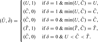The 5 categories above are mutually exclusive and exhaustive.

Under $H_0:F_1(·)=F_2(·)$, note that

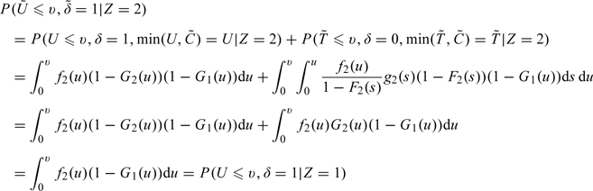and

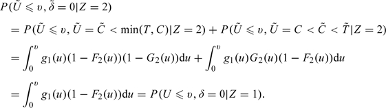Therefore,

(2.1)

for all u and for $j=0,1$. That is, $(\tilde{U},\tilde{\delta })$, formed for group 2 observations, has the same distribution as an observation $(U,\delta )$ from group 1 under H₀. $V_{i2}$ is created in a similar fashion.

By construction, it follows that $V_{i1}$ and $V_{i2}$ are independent of Z_i under H₀. Let V₁ and V₂ denote the n-dimensional column vectors with ith rows $V_{i1}$ and $V_{i2}$, respectively. We then permute the rows of Z while keeping those of $({\mathbf{V}}_1,{\mathbf{V}}_2)$ fixed, resulting in n! matrices $({\mathbf{Z}}^{\left(\mathbf{p}\right)},{\mathbf{V}}_1,{\mathbf{V}}_2)$, where ${\mathbf{Z}}^{\left(\mathbf{p}\right)}$ denotes a row permutation of Z and $p=1,2,\dots ,n!$. Consider a one-to-one transformation from $({\mathbf{Z}}^{\left(\mathbf{p}\right)},{\mathbf{V}}_1,{\mathbf{V}}_2)$ to $({\mathbf{Z}}^{\left(\mathbf{p}\right)},{\mathbf{U}}^{*},{\delta }^{*})$, where

(2.2)

It follows that the n! matrices $({\mathbf{Z}}^{\left(\mathbf{p}\right)},{\mathbf{U}}^{*},{\delta }^{*})$ are equally likely. Note that the original data set corresponds to $(\mathbf{Z},{\mathbf{V}}_1,{\mathbf{V}}_2)$. Thus, if S is any test statistic, an exact permutation test of H₀ can be obtained by comparing the observed value, $S(\mathbf{U},\mathbf{\delta },\mathbf{Z})$, to the permutation distribution of values formed by evaluating S for each of the n! transformed permuted matrices $({\mathbf{Z}}^{\left(\mathbf{p}\right)},{\mathbf{U}}^{*},{\mathbf{\delta }}^{*})$. We denoted this test as ${\text{IP}}_Z(F_1,F_2,G_1,G_2)$ to reflect that it consists of first imputing realizations that depend on $(F_1,F_2,G_1,G_2)$ and then forming permuted data matrices obtained by permuting the rows of Z.

In practice, this test cannot be evaluated because construction of $V_{i1}$ and $V_{i2}$ requires knowledge of $F(·)$, $G_1(·)$, and $G_2(·)$. We recommend that $F(·)$, $G_1(·)$, and $G_2(·)$ be replaced by their respective Kaplan–Meier estimators (Kaplan and Meier, 1958); resulting in IP_Z(, , ₁, ₂). That is, replacing F₁ and F₂ by the Kaplan–Meier estimators of their common value F under H₀ based on the pooled data, and replacing G₁ and G₂ by the their Kaplan–Meier estimators, resulting in an approximate test. Replacing F₁ and F₂ by their individual Kaplan–Meier estimators instead of using for both also yields a valid approximate test. However, because we are interested in the settings where the events in either or both groups are small, ₁ and ₂ will be estimated with less precision, and in some extreme cases where group i has no events, it would be impossible to obtain _i. To create a for an observation $(u,0)$, we first generate a ν from the uniform$(\widehat{F}\left(u\right),1)$ distribution, and then let be ${\widehat{F}}^{-1}\left(\nu \right)\stackrel{\text{def}}{=}\text{inf}\{t:\widehat{F}\left(t\right)\ge \nu \}$. In the event is an incomplete distribution, that is, $\widehat{F}(t_{\text{max}})<1$, and $\nu >\widehat{F}(t_{\text{max}})$, we set $\tilde{t}=t_{\text{max}}$ and consider it to be a censored value, as in Heinze and others (2003). Here, we use $t_{\text{max}}$ to denote the largest observation time. To create a $\tilde{C}\sim G_2(·)$ for an observation in group 1, we first generate a ν from the uniform$(0,1)$ distribution, and then let $\tilde{C}$ be ${\widehat{G}}_2^{-1}\left(\nu \right)$. In the event ${\widehat{G}}_2$ is an incomplete distribution, and $\nu >{\widehat{G}}_2(t_{\text{max},2})$, we set $\tilde{C}$ to be $t_{\text{max}}$. Here, $t_{\text{max},j}$, $j=1,2$ refers to the largest observed time in group j, $j=1,2$. We refer to this approximate test as IP_Z.

2.1.2. Permuting survival times.

Because censoring is noninformative in each group, that is, $T\perp C|Z$, it follows that under $H_0:T\perp Z$, T is independent of $(C,Z)$. Thus, if T were observable, a permutation test $H_0$ could be created by permuting the rows of T while holding those $(\mathbf{C},\mathbf{Z})$ fixed. Since the underlying failure times $T_i,i=1,\dots ,n$ and censoring times $C_i,i=1,\dots ,n$ are not always observed, we employ imputation techniques: consider the n survival times ${\tilde{T}}_i$, $i=1,\dots ,n$, where ${\tilde{T}}_i$ equals $U_i$ when ${\delta }_i=1$ and, when ${\delta }_i=0$, is an independent realization from the conditional distribution, $F_{Z_i}\left(t\right|T>U_i)$, of T, given $T>U_i$ and $Z_i$, for $i=1,\dots ,n$. Similarly, for $i=1,\dots ,n$, define ${\tilde{C}}_i$ to be $U_i$ if ${\delta }_i=0$ and, when ${\delta }_i=1$, is an independent realization from the conditional distribution, $G_{Z_i}\left(t\right|C>U_i)$, of C, given $C>U_i$ and $Z_i$.

To see that ${\tilde{T}}_i$ has unconditional distributions $F_{Z_i}(·)$, suppose $Z_i=1$ so that $T\sim F_1(·)$. Then,

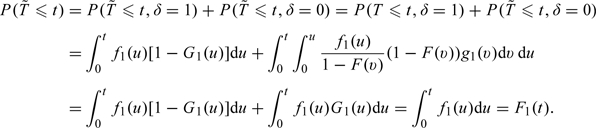Similar arguments apply when $Z_i=0$ and for showing that ${\tilde{C}}_i$ has distribution $G_{Z_i}$.

Let $\tilde{\mathbf{T}}$ and $\tilde{\mathbf{C}}$ denote the corresponding column vectors of length n. Now consider the n × 3 matrix $(\tilde{\mathbf{T}},\tilde{\mathbf{C}},\mathbf{Z})$ and note that under $H_0$, the components of $\tilde{\mathbf{T}}$ are identically distributed and independent of the random variables comprising $(\tilde{\mathbf{C}},\mathbf{Z})$. Thus, an exact permutation test of $H_0$ could be formed analogous to the test described above by permuting the rows of $\tilde{\mathbf{T}}$ while holding the rows of $(\tilde{\mathbf{C}},\mathbf{Z})$ fixed. That is, if $S({\tilde{\mathbf{T}}}^{\left(p\right)},\tilde{\mathbf{C}},\mathbf{Z})$ denotes the value of some test statistic applied to the permuted matrix $({\tilde{\mathbf{T}}}^{\left(p\right)},\tilde{\mathbf{C}},\mathbf{Z})$, an exact p-value for $H_0$ could be calculated by comparing the observed value, $S(\tilde{\mathbf{T}},\tilde{\mathbf{C}},\mathbf{Z})$, to the tail area of the permutation distribution formed by $\left\{S\right({\mathbf{T}}^{\left(p\right)},\tilde{\mathbf{C}},\mathbf{Z}\left)\right|p=1,\dots ,n!\}$. We denote this test ${\text{IP}}_T(F_1,F_2,G_1,G_2)$ to reflect that it consists of an initial imputation step that depends on $(F_1,F_2,G_1,G_2)$ followed by a step in which the survival times are permuted.

In practice, this test cannot be implemented because $F_1(·),F_2(·),G_1(·)$, and $G_2(·)$, used for imputations, are unknown. We recommend that $F(·)$, $G_1(·)$, and $G_2(·)$ be replaced by their respective Kaplan–Meier estimators, yielding an approximate test ${\text{IP}}_T(\widehat{F},\widehat{F},{\widehat{G}}_1,{\widehat{G}}_2)$. In this case, is generated from , the same way as in ${\text{IP}}_Z$. The imputed censoring times ${\tilde{C}}_1$ and ${\tilde{C}}_2$, based on the individual Kaplan–Meier estimators of $G_1(·)$ and $G_2(·)$, respectively, are generated in a similar way, except that when $\nu >{\widehat{G}}_j(t_{\text{max},j})$, we set $\tilde{C}$ to be t_max.

It may appear natural to simply choose a test statistic only depending on $\tilde{\mathbf{T}}$ and Z, as this parallels the usual permutation approach that would be used if the T_i could be observed. However, our experience has been that with small samples and substantial censoring, better performance can be achieved when the test statistic also depends on $\tilde{\mathbf{C}}$ through $(\tilde{\mathbf{U}},\tilde{\mathbf{\delta }})$, where ${\tilde{U}}_i=\text{min}({\tilde{T}}_i,{\tilde{C}}_i)$ and $\widetilde{{\delta }_i}=1$ if ${\tilde{T}}_i\le {\tilde{C}}_i$ and 0 otherwise. For example, for the pth permuted matrix $({\tilde{\mathbf{T}}}^{\left(p\right)},\tilde{\mathbf{C}},\mathbf{Z})$, we can form a log-rank statistic based on the pseudo-data (${\tilde{\mathbf{U}}}^{\left(p\right)}$, ${\tilde{\mathbf{\delta }}}^{\left(p\right)}$, Z), where ${\tilde{U}}_i^{\left(p\right)}=\text{min}({\tilde{T}}_i^{\left(p\right)},{\tilde{C}}_i)$ and ${\tilde{\delta }}_i^{\left(p\right)}=1$ if ${\tilde{T}}_i^{\left(p\right)}\le {\tilde{C}}_i$ and 0 otherwise, and then compare the observed value of S to the permutation distribution of n! possible values. When $F_1(·)\ne F_2(·)$, the treatment difference in survival times manifested in the original data set $(U,\delta ,Z)$ might be attenuated if we obtain the observed test statistic from $(\tilde{T},Z)$ because a proportion of is obtained from the common . The magnitude of attenuation would depend on the amount of censoring, which determines the proportion of that needs to be imputed. Furthermore, as one reviewer has pointed out, this approach is “too imputation dependent” in the sense that even the observed test statistic would be different depending on the employed imputations, which makes this approach of little value in practice.

2.1.3. Multiple imputations.

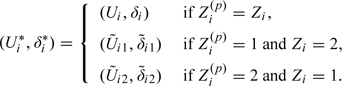
In the 2 imputation–permutation methods described above, we can view the observed data as incomplete data and the imputation step attempts to create complete data for the subsequent permutation step. Let y denote the observed data $(\mathbf{Z},\mathbf{U},\mathbf{\delta })$. The complete data x is $(\mathbf{Z},{\mathbf{V}}_1,{\mathbf{V}}_2)$ for IP_Z and $(\mathbf{Z},\tilde{\mathbf{T}},\tilde{\mathbf{C}})$ for IP_T. 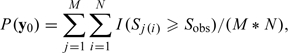Let and denote the sample spaces corresponding to x and y. There is a many-to-one mapping $\mathbf{x}\to \mathbf{y}\left(\mathbf{x}\right)$ from and . Let $A({\mathbf{y}}_0)=\{\mathbf{x}\in 𝒳:\mathbf{y}\left(\mathbf{x}\right)={\mathbf{y}}_0\}$, which is the collection of all complete data sets that are consistent with an observed ${\mathbf{y}}_0$. Let $h\left(\mathbf{x}\right)$ denote the sampling density for x. The imputations in $A({\mathbf{y}}_0)$ are independently and identically distributed with density $h\left(\mathbf{x}\right)I(\mathbf{x}\in A({\mathbf{y}}_0\left)\right)/P(\mathbf{x}\in A({\mathbf{y}}_0\left)\right)$. Let $B\left(\mathbf{x}\right)=\{{\mathbf{x}}^{*}:{\mathbf{x}}^{*}\text{is\hspace{0.5em}a\hspace{0.5em}permutation\hspace{0.5em}of}\mathbf{x}\}$. Let $C({\mathbf{y}}_0)$ be the union of the B(x) over x in $A({\mathbf{y}}_0)$, which gives all complete data sets that can be obtained as a permutation of a complete data set that is consistent with ${\mathbf{y}}_0$. Finally, let $D({\mathbf{y}}_0)=\{\mathbf{y}:\mathbf{y}=\mathbf{y}\left(\mathbf{x}\right)\text{for\hspace{0.5em}some\hspace{0.5em}randomly\hspace{0.5em}selected}\mathbf{\hspace{0.5em}x}\text{\hspace{0.5em}in}C({\mathbf{y}}_0\left)\right\}$, which is the reduction of the complete data sets in $C\left({\mathbf{y}}_0\right)$ to observable data sets. For both IP_Z and IP_T, we are trying to make inferences conditional on y in $D({\mathbf{y}}_0)$; that is, on y being obtained from a permutation of a complete data set consistent with the observed data. However, this conditional reference set does not give a distribution-free test, as reflected in the need to specify a distribution for the imputations. Let M denote the number of imputations sampled from $A({\mathbf{y}}_0)$, and let N denote the number of permutations per imputation. In Sections 2.1.1 and 2.1.2, we show that for each imputation, when imputed from the true distribution, the N permutations are equally likely as the observed data under the null hypothesis. Therefore, we can view y₀ as a random sample of size 1 from $D({\mathbf{y}}_0)$. The one-sided p-value corresponding to the observed data set y₀ takes the form

(2.3)

where S_obs denote the observed test statistic and $S_{j\left(i\right)}$ denote the test statistic evaluated on the reduced permuted imputed data set for $j=1,\cdots ,M$ and $i=1,\cdots ,N$. In practice, although when imputing from the true distributions F, G₁, and G₂, the p-value obtained from IP_Z or IP_T based on one single imputation would follow a uniform distribution and leads to valid inference, its interpretation depends on a specific imputation. Note that (2.3) can also be viewed as the average of M p-values, each obtained from a single imputation and N permutations. Multiple imputation eliminates the problem of reliance on a single imputation and can be viewed as an approximation to the expectation of the p-values obtained from the complete data conditional on the observed data.

The approach in Heinze and others (2003) coincides with IP_T for the case $M>1$ and N = 1. That is, we perform multiple imputations and one permutation for each imputation is included in $D({\mathbf{y}}_0)$. Heinze and others (2003) describe their approach by first permuting $(\tilde{\mathbf{U}},\mathbf{\delta })$ (step 3), and creating $\tilde{\mathbf{T}}$ and $\tilde{\mathbf{C}}$ by imputation (step 4). We first note that $\tilde{\mathbf{C}}$ is created from the observed data set and does not involve the permuted data set. Therefore, it can be created before the permutation as in IPT. For $\tilde{\mathbf{T}}$, although the indices of $(U_i,{\delta }_i)$ change after permutation, because it is imputed from the common , switching the group membership does not affect the imputation. Therefore, $\tilde{\mathbf{T}}$ can also be created before the permutation as in IP_T. That is, one initially generates multiple imputed values of the vectors $\tilde{\mathbf{T}}$ and $\tilde{\mathbf{C}}$, and then for the pth permutation, creates a permuted data matrix based on the pth $\tilde{\mathbf{T}}$ while holding Z and the pth $\tilde{\mathbf{C}}$ fixed. One can then use this data matrix to evaluate the test statistic. This would yield the test in Heinze and others (2003).

2.2. Point and interval estimation

When a semiparametric or parametric model is postulated for how the survival distributions of the 2 groups differ, then methods proposed in Section 2.1 can be inverted to obtain point and interval estimates for the model parameters. We consider the AFT model: specifically, if $T_1$ and $T_2$ denote survival times from $F_1(·)$ and $F_2(·)$, respectively, and $\beta >0$ is some positive constant, then $T_1$ has the same distribution as $\beta T_2$; equivalently, $F_2\left(t\right)=F_1\left(\beta t\right)$. Thus, β characterizes the difference between the underlying survival distributions in the 2 groups and $H_0:F_1(·)=F_2(·)$ is equivalent to $H_0:\beta =1$. If $\beta >1(<1)$, then $T_1$ is stochastically larger (smaller) than $T_2$. Note that under an AFT model, the hazards for the 2 groups are in general nonproportional, with the exception being when the groups have Weibull survival distributions with the same shape parameter (and thus also when they both have exponential survivals), in which case $h_2\left(t\right)=\beta h_1\left(\beta t\right)$.

Consider an observation, say $(U_1,{\delta }_1)$ from group 1, and recall that this arises as $U_1=\text{min}(T_1,C_1)$ and ${\delta }_1=1$ if $T_1\le C_1$ and 0 otherwise. Under an AFT model, $U_1^{*}=U_1/\beta =\text{min}(T_1/\beta ,C_1/\beta )=\text{min}(T_1^{*},C_1^{*})$, where $T_1^{*}$ has distribution function $F_1\left(\beta t\right)=F_2\left(t\right)$ and $C_1^{*}$ has distribution function $G_1\left(\beta t\right)$. Thus, if the $i$th observation, say $(U_i,{\delta }_i)$ in group 1 were transformed to $(U_i^{*},{\delta }_i)=(U_i/\beta ,{\delta }_i)$, the result would be an observation from an underlying survival distribution $F_2\left(t\right)$ and underlying censoring distribution $G_1\left(\beta t\right)$.

To use these results to construct a confidence interval for β, let ${\beta }_0$ be some specified value and consider testing $H({\beta }_0):\beta ={\beta }_0$. Let $(U^{*},\delta ,Z)$ denote the data matrix obtained by replacing those $U_i$ for subjects in group 1 by $U_i/{\beta }_0$. Then under $H({\beta }_0)$, the transformed data arise from 2 groups with equal underlying survival distributions and, in general, different underlying censoring distributions. It follows that the methods in Section 2.1 can be used to construct a test of $H({\beta }_0)$ for any ${\beta }_0$. A confidence interval of size $100(1-\alpha )$% for β can then be formed by the set of ${\beta }_0$ which are not rejected at the α level of significance. These intervals would be exact if the tests in Section 2.1 were imputed from the true underlying distributions $(F_1,F_2,G_1,G_2)$ but in practice would be approximate because Kaplan–Meier estimators would be used. A point estimate for β is given by the value for which there is the least evidence against $H({\beta }_0):\beta ={\beta }_0$, say, by giving the largest p-value. In the absence of censoring observations, the confidence intervals obtained from inverting both IP_T and IP_Z yield the same results as the Hodges and Lehmann interval estimates of the location shift for underlying survival times on the log scale (Hodges and Lehmann, 1963).

3. SIMULATION RESULTS

We begin this section by presenting simulation studies to assess the performance of IP_T and IP_Z for testing hypotheses and to compare these to the method of Heinze and others (2003). We then assess the coverage probabilities of the proposed methods for interval estimation and compare these to coverage probabilities from the semiparametric approach of Jin and others (2003).

Empirical Type 1 errors and power are based on 2000 replications of studies. For each setting, we performed one imputation to prepare the data set for permutation and then randomly generated 1000 permutations rather than enumerating all n! possible permutations. For ease of comparisons, simulations were done first using the settings as in Heinze and others (2003), where (1) the sample sizes for 2 groups are $(6,6)$, $(6,30)$, $(30,30)$, and $(3,120)$, (2) censoring times are generated as the minimum of a realization from uniform $(12,60)$ reflecting administrative censoring and a realization from an exponential distribution with hazard rate ${\gamma }_1$ and ${\gamma }_2$ for groups 1 and 2, respectively, reflecting potential times until loss to follow up, and (3) the underlying failure times are from an exponential distribution with hazard rates ${\lambda }_1$ and ${\lambda }_2$. For IP_T and IP_Z, the test statistic we used was the numerator of the log-rank statistic, as in Heinze and others (2003). The results are displayed in Table 1 (empirical Type 1 error) and Table 2 (power) for the log-rank test (“Log-rank”), ordinary permutation test (“Perm”) which requires equal underlying censoring distributions, the test in Heinze and others (“Heinze”), and the 2 proposed tests (“IP_T” and “IP_Z”). We also examined the performance of IP_T and IP_Z, where and $\tilde{C}$ are imputed from the true survival and censoring distributions F, $G_1$, and $G_2$ (“IP_T^*” and “IP_Z^*”). In Table 2, where $F_1\ne F_2$, the common F is taken to be a mixture distribution of $F_1$ and $F_2$ with the mixture probabilities proportional to the sample sizes in the 2 groups. The results for the Log-rank, Perm, and Heinze methods are taken from Heinze and others (2003). As shown in Heinze and others (2003), the Type I errors for the log-rank test become distorted with very small sample sizes and/or unequal censoring distributions, and those for the ordinary permutation test become distorted when the underlying censoring distributions differ. In contrast, the Type 1 errors of the Heinze test and the 2 proposed tests are relatively close to nominal levels for all settings. The empirical powers of the 2 proposed tests are generally similar to those of the Heinze test. Imputing from the Kaplan–Meier estimates , ${\widehat{G}}_1$, and ${\widehat{G}}_2$ yield very similar results as imputing from the true F, $G_1$, and $G_2$, both in terms of Type I error and power. We will return to this point in Section 5.

Table 1.

Empirical Type I error estimates for one-sided 0.05 level test of equal survival (H₀: F₁(t) = F₂(t)) against shorter/longer survival of group 1 versus group 2 (H₁:F₁(t) > F₂(t)/H₁: F₁(t) < F₂(t)), F₁(t) = F₂(t) ∼ exp(0.04), c₁ and c₂ refer to the percentages of censored observations

n1	n2	γ1	γ2	c1† (%)	c2† (%)	Log-rank†	Perm†	Heinze†	IPT	IPT*	IPZ	IPZ*
6	6	0.00	0.00	27.5	27.6	0.056/0.057	0.049/0.052	0.048/0.050	0.060/0.054	0.052/0.048	0.052/0.046	0.047/0.057
6	6	0.04	0.04	54.5	54.7	0.057/0.055	0.051/0.049	0.053/0.053	0.049/0.045	0.055/0.050	0.044/0.049	0.044/0.049
30	30	0.00	0.00	27.5	27.5	0.050/0.053	0.049/0.050	0.046/0.048	0.055/0.051	0.047/0.062	0.050/0.049	0.048/0.051
30	30	0.04	0.04	54.9	54.8	0.049/0.052	0.047/0.050	0.047/0.050	0.057/0.062	0.046/0.049	0.051/0.050	0.048/0.048
6	30	0.00	0.00	27.5	27.5	0.078/0.035	0.049/0.048	0.045/0.047	0.049/0.057	0.050/0.058	0.053/0.053	0.056/0.046
6	30	0.04	0.04	54.9	54.8	0.077/0.034	0.049/0.050	0.048/0.050	0.052/0.052	0.051/0.047	0.057/0.043	0.052/0.042
3	120	0.00	0.00	27.3	27.5	0.113/0.025	0.050/0.049	0.050/0.043	0.049/0.051	0.059/0.049	0.047/0.051	0.062/0.037
3	120	0.04	0.04	54.6	54.9	0.109/0.013	0.050/0.050	0.050/0.031	0.052/0.051	0.045/0.045	0.040/0.041	0.057/0.048
6	6	0.00	0.04	27.4	54.9	0.047/0.063	0.048/0.039	0.048/0.051	0.051/0.051	0.047/0.045	0.048/0.037	0.051/0.045
30	30	0.00	0.04	27.5	54.8	0.045/0.055	0.045/0.038	0.046/0.047	0.053/0.060	0.046/0.042	0.049/0.045	0.052/0.047
6	30	0.00	0.04	27.5	54.8	0.071/0.040	0.075/0.068	0.047/0.051	0.054/0.059	0.053/0.053	0.058/0.048	0.048/0.048
6	30	0.04	0.00	54.9	27.5	0.081/0.030	0.023/0.025	0.047/0.043	0.045/0.054	0.045/0.048	0.056/0.056	0.054/0.053
3	120	0.00	0.04	27.3	54.9	0.110/0.027	0.100/0.094	0.050/0.051	0.050/0.053	0.054/0.045	0.051/0.057	0.049/0.041
3	120	0.04	0.00	54.6	27.5	0.110/0.012	0.028/0.016	0.046/0.019	0.054/0.046	0.048/0.046	0.046/0.040	0.045/0.056

^*Imputed from the true underlying F, G₁, and G₂.

^†Taken from Heinze and others (2003).

Table 2.

Empirical power estimates for one-sided 0.05 level test of equal survival (H₀:F₁(t) = F₂(t)) against shorter/longer survival of group 1 versus group 2 (H₁: F₁(t) > F₂(t)/H₁:F₁(t) < F₂(t)), F_j(t) ∼ exp(λ_j), j = 1, 2, (λ₁, λ₂) = (0.08, 0.04)/(0.04, 0.08), c₁ and c₂ refer to the percentages of censored observations

n1	n2	γ1	γ2	c1† (%)	c2† (%)	Log-rank†	Perm†	Heinze†	IPT	IPT*	IPZ	IPZ*
6	6	0.00	0.00	10/28	27/10	0.280/0.277	0.254/0.252	0.248/0.247	0.256/0.257	0.257/0.256	0.242/0.252	0.254/0.252
6	6	0.04	0.04	37/55	54/35	0.213/0.210	0.197/0.196	0.198/0.198	0.221/0.203	0.176/0.181	0.192/0.185	0.163/0.185
30	30	0.00	0.00	10/27	27/10	0.772/0.773	0.762/0.765	0.758/0.759	0.786/0.766	0.773/0.768	0.758/0.772	0.729/0.760
30	30	0.04	0.04	36/55	55/36	0.615/0.616	0.605/0.608	0.603/0.605	0.640/0.600	0.608/0.609	0.578/0.556	0.548/0.540
6	30	0.00	0.00	10/27	27/10	0.459/0.348	0.355/0.397	0.336/0.396	0.336/0.437	0.350/0.393	0.343/0.399	0.350/0.384
6	30	0.04	0.04	36/54	55/36	0.366/0.242	0.282/0.291	0.278/0.292	0.270/0.312	0.261/0.280	0.264/0.286	0.258/0.279
3	120	0.00	0.00	10/28	28/10	0.407/0.221	0.223/0.309	0.222/0.306	0.215/0.312	0.223/0.307	0.211/0.317	0.230/0.286
3	120	0.04	0.04	37/54	55/36	0.342/0.137	0.196/0.223	0.193/0.204	0.180/0.231	0.190/0.191	0.159/0.227	0.190/0.237
6	6	0.00	0.04	10/27	54/36	—‡	—	0.223/0.211	0.241/0.208	0.210/0.211	0.221/0.196	0.196/0.194
30	30	0.00	0.04	10/27	55/36	—	—	0.676/0.654	0.697/0.659	0.690/0.638	0.653/0.619	0.650/0.637
6	30	0.00	0.04	10/27	55/36	—	—	0.329/0.351	0.340/0.392	0.332/0.341	0.339/0.348	0.323/0.351
6	30	0.04	0.00	37/55	28/10	—	—	0.277/0.313	0.261/0.319	0.278/0.313	0.271/0.280	0.293/0.286
3	120	0.00	0.04	10/27	55/36	—	—	0.223/0.298	0.225/0.311	0.211/0.305	0.236/0.296	0.212/0.296
3	120	0.04	0.00	36/55	28/10	—	—	0.177/0.198	0.183/0.223	0.179/0.226	0.186/0.229	0.190/0.245

^*imputed from the true underlying F, G₁, and G₂.

^‡“—” indicates settings where the corresponding tests are not expected to maintain the nominal Type I error rates.

^†Taken from Heinze and others (2003).

Tables 3 presents empirical coverage probabilities for nominal 95% confidence intervals of the AFT parameter β (Section 2.2) obtained from the semiparametric approach in Jin and others (2003), denoted “Jin,” and based on the proposed methods, with varying $F_1(·)$ and $F_2(·)$, sample sizes, and amount of censoring. In addition, we evaluated performance of a variation of Jin's method where a bootstrap method was used for estimating variance, denoted as “Jin^*.” The actual coverage probabilities of Jin (or Jin^*) can be substantially lower than the nominal level 95% when the sample sizes (or number of events) are small. In contrast, the coverage probabilities from the proposed methods are usually close to the nominal level. We also compare the performance of Jin and the proposed methods when sample sizes are large (Table 4). Here, the actual coverage of all methods is in general close to the nominal level. The confidence intervals formed by the proposed methods have similar median width as the Jin's method.

Table 3.

Actual coverage of nominal 95% confidence interval using Jin, IP_T, and IP_Z for β in the AFT model: F₂(t) = F₁(βt), where β = 2, c₁ and c₂ refer to the percentages of censored observations in groups 1 and 2, respectively

Uniform(12, 60)
				log(T1) ∼ logistic(0, 1)						log(T1) ∼ N(3, 1)
n1	n2	γ1	γ2	c1 (%)	c2 (%)	Jin (%)	Jin* (%)	IPT (%)	IPZ (%)	c1 (%)	c2 (%)	Jin (%)	Jin* (%)	IPT (%)	IPZ (%)
10	10	0.12	0.04	22	18	92.6	91.6	95	95	83	79	78.6	90.0	98	98
10	10	0.04	0.04	12	18	92.0	90.4	95	95	61	80	86.0	89.6	97	95
10	10	0.00	0.04	3	18	91.6	90.4	93	95	32	79	85.0	87.2	97	96
10	10	0.00	0.00	3	6	90.8	90.0	95	95	32	57	91.4	91.8	94	94
10	50	0.00	0.04	3	18	95.0	92.0	95	96	32	79	90.8	92.6	95	95
Uniform(12, 60)
				log(T1) ∼ logistic(0, 1)						log(T1) ∼ N(0, 1)
n1	n2	γ1	γ2	c1 (%)	c2 (%)	Jin (%)	Jin* (%)	IPT (%)	IPZ (%)	c1 (%)	c2 (%)	Jin (%)	Jin* (%)	IPT (%)	IPZ (%)
10	10	1.5	1.5	67	79	81.8	85.6	96	97	72	86	71.6	85.8	96	98
10	10	1	1	60	72	89.8	91.8	94	96	62	78	83.4	88.6	96	96
20	10	1.5	1.2	67	75	91.0	91.8	96	95	72	82	81.6	85.2	96	97
50	10	1.5	1.2	67	75	93.8	91.2	95	95	72	82	88.8	82.6	96	98
50	50	1.5	1.5	67	79	96.0	96.0	95	97	72	86	94.8	97.2	96	97
Uniform(0.5, 2)
				log(T1) ∼ logistic(0, 1)						log(T1) ∼ N(0, 1)
n1	n2	γ1	γ2	c1 (%)	c2 (%)	Jin (%)	Jin* (%)	IPT (%)	IPZ (%)	c1 (%)	c2 (%)	Jin (%)	Jin* (%)	IPT (%)	IPZ (%)
10	10	1	1	64	77	84.4	87.4	97	95	68	85	75.8	84.8	95	97
20	10	1.5	1	69	77	90.2	91.4	97	96	75	85	76.4	79.6	97	98
50	10	1.5	1	69	77	92.6	88.8	96	97	75	85	79.8	75.4	95	97
50	50	1.5	1	69	77	96.8	96.0	95	95	75	85	94.6	96.8	95	97
10	10	0	0	46	63	90.6	91.6	96	94	44	70	90.6	90.6	95	96

^*Variance estimates obtained using bootstrap.

Table 4.

Actual coverage and median width of nominal 95% confidence interval using Jin, IP_T, and IP_Z for β in the AFT model: F₂(t) = F₁(βt), where β = 2, c₁ and c₂ refer to the percentages of censored observations in groups 1 and 2, respectively

Uniform(12, 60), log(T1) ∼ logistic(0, 1)
n1	n2	γ1	γ2	c1 (%)	c2 (%)	Jin		IPT		IPZ
50	50	0.00	0.04	3	18	92.2%,	1.37	94.2%,	1.55	95.6%,	1.54
50	100	0.00	0.04	3	18	91.0%,	1.21	94.4%,	1.33	95.4%,	1.33
100	50	0.00	0.04	3	18	94.2%,	1.33	96.0%,	1.33	95.0%,	1.32
100	100	0.00	0.04	3	18	95.8%,	1.10	94.6%,	1.09	95.0%,	1.08
Uniform(12, 60), log(T1) ∼ N(3, 1)
n1	n2	γ1	γ2	c1 (%)	c2 (%)	Jin		IPT		IPZ
50	50	0.00	0.04	32	79	93.4%,	1.06	94.8%,	1.13	96.2%,	1.15
50	100	0.00	0.04	32	79	95.0%,	0.88	96.2%,	0.93	96.4%,	0.94
100	50	0.00	0.04	32	79	96.6%,	1.00	96.0%,	1.00	94.4%,	1.02
100	100	0.00	0.04	32	79	95.2%,	0.79	94.8%,	0.78	93.8%,	0.81
Uniform(12, 60), log(T1) ∼ logistic(0, 1)
n1	n2	γ1	γ2	c1 (%)	c2 (%)	Jin		IPT		IPZ
50	50	1.5	1.5	67	79	93.6%,	2.05	94.8%,	2.12	96.0%,	2.19
50	100	1.5	1.5	67	79	94.8%,	1.72	95.4%,	1.73	94.8%,	1.79
100	50	1.5	1.5	67	79	97.4%,	1.81	95.6%,	1.80	95.2%,	1.83
100	100	1.5	1.5	67	79	94.4%,	1.43	95.8%,	1.44	94.8%,	1.48
Uniform(12, 60), log(T1) ∼ N(0, 1)
n1	n2	γ1	γ2	c1 (%)	c2 (%)	Jin		IPT		IPZ
50	50	1.5	1.5	72	86	94.0%,	1.39	95.4%,	1.34	97.6%,	1.15
50	100	1.5	1.5	72	86	93.8%,	1.13	94.4%,	1.12	95.6%,	1.26
100	50	1.5	1.5	72	86	95.4%,	1.26	94.4%,	1.20	93.4%,	1.30
100	100	1.5	1.5	72	86	93.2%,	0.98	95.8%,	0.96	95.6%,	1.04
Uniform(0.5, 2), log(T1) ∼ logistic(0, 1)
n1	n2	γ1	γ2	c1 (%)	c2 (%)	Jin		IPT		IPZ
50	50	1.5	1	69	77	95.4%,	1.93	94.4%,	2.00	95.0%,	2.07
50	100	1.5	1	69	77	93.6%,	1.63	95.6%,	1.68	95.4%,	1.71
100	50	1.5	1	69	77	97.4%,	1.71	93.4%,	1.73	92.4%,	1.76
100	100	1.5	1	69	77	96.4%,	1.36	97.0%,	1.35	95.2%,	1.41
Uniform(0.5, 2), log(T1) ∼ N(0, 1)
n1	n2	γ1	γ2	c1 (%)	c2 (%)	Jin		IPT		IPZ
50	50	1.5	1	75	85	94.6%,	1.28	96.0%,	1.32	95.8%,	1.41
50	100	1.5	1	75	85	95.6%,	1.06	94.2%,	1.13	95.8%,	1.14
100	50	1.5	1	75	85	95.2%,	1.13	95.8%,	1.15	94.2%,	1.21
100	100	1.5	1	75	85	94.2%,	0.91	94.4%,	0.91	95.6%,	0.95

4. EXAMPLES

4.1. Survival following breast cancer

We first illustrate the proposed methods with the example used in Heinze (2002), which compares the survival of breast cancer patients who had primary treatment at the Department of Surgery of the University Hospital in Vienna between 1982 and 2001 and had either been enrolled in clinical trials (the “trial” group) or not (the “nontrial” group). The group sizes were 38 (all censored) for the trial group and 90 (80 censored) for the nontrial group. The median (quartiles) of follow-up time were 9.5 (5.8–24.3) and 79.1 (56.0–98.7), respectively, suggesting unequal underlying censoring distributions.

As noted in Heinze and others (2003), use of Heinze and Log-rank give one-sided p-values of 0.031 and 0.05, suggesting that breast cancer patients enrolled in a clinical study experience longer survival. The one-sided p-values are 0.023 using IP_T and 0.075 using IP_Z, based on 10 000 imputation–permutations. Previous analyses of these data have focused on testing and not on interval estimation. To quantify the difference in survival times between 2 groups of cancer patients, we then fit AFT models and obtained 95% one-sided confidence intervals for β, the ratio of a typical underlying survival time in the trial group to one in the nontrial group, of (1.06, ∞) using IP_T and (0.66, ∞) using IP_Z. The upper limits in both cases reflect the fact that all observations in the trial group were censored. Jin's method failed to provide a point estimate or an interval estimate because there were no events in the trial group.

4.2. Virologic progression and survival in HIV-infected infants

We then apply the proposed methods to data from a recent AIDS study (Lockman and others, 2007). One of the main study objectives was to investigate whether a single dose of nevirapine (NVP) leads to viral NVP resistance mutations in infants. The primary end point for infants was virologic failure within 6 months after initiating antiretroviral treatment (ART). Among thirty infants who started ART, one out of the fifteen randomized to placebo group and ten out of the fifteen randomized to single NVP group reached the primary end point (Figure 1(a)). Figure 1(b) plots the IP_T and IP_Z p-values for testing various hypothesis $H_0:\beta ={\beta }_0$, where β₀ ranges from 0.0001 to 1.5. For IP_T, we obtain a point estimate of $\widehat{\beta }=0.43$ and 95% confidence interval (0, 0.83). IP_Z gives the same point estimate and a 95% confidence interval (0, 0.84). Jin's method gives the same point estimate but with a shorter nominal confidence interval (0.27, 0.70). Because this is a setting where one group had only one event, the simulation studies from Section 3 would suggest that the coverage of Jin's method may be substantially lower than the nominal level. Consequently, the confidence intervals obtained from inverting IP_T or IP_Z are more likely to reflect the true uncertainty associated with the point estimate.

Fig. 1.

Time to virologic failure. (a): Kaplan-Meier estimates for time to virologic failure, by treatment group; (b): the average of 10 p-values for testing $H_0:\beta ={\beta }_0$ for various ${\beta }_0\in (0,1.5)$. Solid: IP_T; Dashed: IP_Z; Dotdashed: a horizontal line at 0.05.

A secondary end point for infants was time until the composite end point of either virologic failure or death. Four infants from the placebo group and eleven from the single NVP group had this composite end point. The Kaplan–Meier estimates are presented in Figure 2(a). In this case, inverting IP_T yields a point estimate of $\widehat{\beta }=0.60$ with a 95% confidence interval of (0.19, 1.02); inverting IP_Z yields the same point estimate and a slightly wider confidence interval of (0.19, 1.07) (Figure 2(b)). The Jin's method gives a point estimate of 0.58 and a 95% confidence interval of (0.28, 1.19). The point estimates from IP_T, IP_Z, and the Jin's method are again very similar. The intervals obtained through inverting IP_T or IP_Z, somewhat shifted to the left, are slightly shorter in length than the interval obtained through Jin's, suggesting that the proposed procedures have similar efficiency as those of Jin and others for settings like this, where the number of events is not extremely small.

Fig. 2.

Time to virologic failure or death. (a): Kaplan-Meier estimates for time to virologic failure or death, by treatment group; (b): the average of 10 p-values for testing $H_0:\beta ={\beta }_0$ for various ${\beta }_0\in (0,1.5)$. Solid: IP_T; Dashed: IP_Z; Dotdashed: a horizontal line at 0.05.

5. DISCUSSION

Motivated by the poor performance of the log-rank test in settings where the sample sizes in one or both groups is small and where the underlying censoring distributions of the groups may differ, and by the lack of interval estimation methods for such settings, we develop 2 methods by adapting hypothetical permutation methods that could be used when the censoring distributions in 2 groups were equal or when the underlying survival and censoring times were known. One of the methods coincides with the approach of Heinze and others (2003) when imputation is performed for each permutation. We examined cases with very small sample sizes in one or both groups (e.g. 6 versus 6, 3 versus 120). In such settings, the Kaplan–Meier estimator of F or G cannot be expected to be accurate. However, the tests still maintain very good Type I error rates. More interestingly, the Type I error and power of the proposed methods are very similar to those obtained when imputing from the true F and G. This may be partly due to the fact that each imputed permuted data set may only involves a small portion of imputed values. When comparing the permuted imputed failure times and censoring times, extra variation due to imputing from estimated distributions only comes into play when the minimum of the 2 happens to be the imputed value. In addition, this could happen only to the rows of the data matrix affected by a particular permutation.

The proposed methods readily provide confidence intervals for the group difference under an AFT model. The large-sample method of Jin and others (2003) is seen to sometimes have poor coverage probabilities in small-sample settings. In contrast, the coverage probabilities of the proposed methods are generally close to nominal levels in the simulation studies we examined. In addition, the proposed methods are seen to be as efficient as the Jin's method in large-sample settings.

In all the settings we examined, IP_T and IP_Z have similar performance with respect to Type I error, power and required computing time. Therefore, we do not prefer one over the other. For the permutation step, IP_Z only requires T ⊥ Z, while IP_T requires both T ⊥ Z and $T\perp C|Z$. However, for the imputation step because we use the Kaplan–Meier estimates of F, $G_1$, and $G_2$, the independent censoring assumption $T\perp C|Z$ is required for both. For IP_Z, the imputation for the censoring times only uses information from the censoring distribution of the other group; while for IP_T, the imputation for the censoring times depends on both the censoring distribution of the same group, as well as the observed survival times. As with any statistical method that uses imputation, for IP_T and IP_Z, the resulting p-values will depend in part on the random number generators and seeds used to impute. We recommend the use of multiple imputations and the number of imputations should be large enough to adequately control the dependence on the specific imputations. For a particular setting, although imputations can be completely enumerated in theory, the number of possible imputations increases as the number of observations increases and it is often not necessary to enumerate all imputations in practice. For each imputation, there are a large number of associated permutations. In our example in Section 4.2, we used 10 imputations and 2000 permutations for each imputation. The p-value curves for both IP_T and IP_Z in Figure 2(b) appeared to be reasonably smooth, suggesting that 10 imputations were sufficient in this case. This observation is in line with recommendations on the number of imputations needed in other multiple imputation settings. For example, Rubin (1987) argued that more than 10 imputations would rarely be needed.

Although we focus our discussion on testing $H_0:F_1(·)=F_2(·)$, the proposed methods also apply for testing other null hypotheses. For example, if our main interest were in the cumulative survival probability at a specific time point, say, 1 year, then we could use IP_T and IP_Z with a test statistic based on the difference between the Kaplan–Meier estimators of the 2 groups at 1 year. Note that for this hypothesis and particular choice of test statistic, the influence of imprecision resulting from having to impute the $\tilde{T}$ and $\tilde{C}$ from an incomplete distribution would be reduced because the test statistic is invariant to specific values of observations larger than 1 year.

It would also be useful to evaluate how the performances of IP_Z and IP_T are affected by different choices of test statistics. The imputation–permutation principle in IP_T and IP_Z can be extended to the class of weighted log-rank statistics, such as Prentice's test (Prentice, 1978). We used the numerator of the log-rank test so that the results were directly comparable to Heinze and others (2003). Different test statistics were used in Troendle and Yu (2006). Neuhaus (1993) examined the asymptotic properties of the standard permutation test and found that, when a standardized test statistic is used, the resulting permutation test is strictly distribution free under the null hypothesis if the censoring distributions are equal in both groups and asymptotically equivalent to their unconditional counterparts when the censoring distributions are different. We assessed the performance of using a standardized test statistic in finite-sample settings and did not observe consistent improvement in the settings examined.

The proposed methods can readily be generalized for the comparison of more than 2 groups. In addition, they can be generalized to allow stratified analyses, analogous to the stratified log-rank test, by using a restricted set of permutations. For example, to adapt the proposed methods to compare treatment groups while stratifying by sex, one need only (1) use a test statistic that reflects the stratification, such as the numerator of the stratified log-rank test and (2) only consider those permutations in which the rows of the permuted values of survival or group membership lead to the same gender as the original data matrix. Although our focus in interval estimation was on AFT models, the IP_T and IP_Z tests can, in principle, be inverted to obtain confidence regions for parameters in other semiparametric models such as the changing shape and scale model (Bagdonavičius and others, 2004).

FUNDING

National Institutes of Health (R37 AI24643, T32 AI007358).

References

- Bagdonavičius V, Cheminade O, Nikulin M. Statistical planning and inference in accelerated life testing using the CHSS model. Journal of Statistical Planning and Inference. 2004;126:535–551. [Google Scholar]
- Breslow NE. A generalized Kruskal-Wallis test for comparing K-samples subject to unequal patterns of censoring. Biometrika. 1970;57:579–594. [Google Scholar]
- Cox DR. Regression models and life-tables (with discussion) Journal of the Royal Statistical Society, Series B. 1972;34:187–220. [Google Scholar]
- Dirienzo AG, Lagakos SW. Effects of model misspecification on tests of no randomized treatment effect arising from Cox's proportional hazards model. Journal of the Royal Statistical Society, Series B. 2001;63:745–757. [Google Scholar]
- Heimann G, Neuhaus G. Permutational distribution of the log-rank statistic under random censorship with applications to carcinogenicity assays. Biometrics. 1998;54:168–184. [PubMed] [Google Scholar]
- Heinze G. Section of Clinical Biometrics. Vienna, Austria: University of Vienna; 2002. Exact linear rank tests for possibly heterogeneous follow-up. Technical Report 08/2002. Department of Medical Computer Sciences. [Google Scholar]
- Heinze G, Gnant M, Schemper M. Exact log-rank tests for unequal follow-up. Biometrics. 2003;59:1151–1157. doi: 10.1111/j.0006-341x.2003.00132.x. [DOI] [PubMed] [Google Scholar]
- Hodges JL, Lehmann EL. Estimates of location based on rank tests. Annals of Mathematical Statistics. 1963;34:598–611. [Google Scholar]
- Jennrich RI. Some exact tests for comparing survival curves in the presence of unequal right censoring. Biometrika. 1984;71:57–64. [Google Scholar]
- Jin Z, Lin DY, Wei LJ, Ying Z. Rank-based inference for the accelerated failure time model. Biometrika. 2003;90:341–353. [Google Scholar]
- Johnson ME, Tolley HD, Bryson MC, Goldman AS. Covariate analysis of survival data: a small-sample study of Cox's model. Biometrics. 1982;38:685–698. [PubMed] [Google Scholar]
- Jones MP, Crowley J. A general class of nonparametric tests for survival analysis. Biometrics. 1989;45:157–170. [PubMed] [Google Scholar]
- Kaplan AM, Meier P. Nonparametric estimation from incomplete observations. Journal of the American Statistical Association. 1958;53:457–481. [Google Scholar]
- Kellerer AM, Chmelevsky D. Small-sample properties of censored-data rank tests. Biometrics. 1983;39:675–682. [Google Scholar]
- Klein JP, Moeschberger ML. Survival Analysis: Techniques for Censored and Truncated Data. 2nd edition. New York: Springer; 2003. [Google Scholar]
- Kong FH, Slud E. Robust covariate-adjusted logrank tests. Biometrika. 1997;84:847–862. [Google Scholar]
- Latta RB. A Monte Carlo study of some two-sample rank tests with censored data. Journal of the American Statistical Association. 1981;76:713–719. [Google Scholar]
- Lockman S, Shapiro RL, Smeaton LM, Wester C, Thior I, Stevens L, Chand F, Makhema J, Moffat C, Asmelash A. and others. Response to antiretroviral therapy after a single, peripartum dose of nevirapine. The New England Journal of Medicine. 2007;356:135–147. doi: 10.1056/NEJMoa062876. [DOI] [PubMed] [Google Scholar]
- Louis TA. Nonparametric analysis of an accelerated failure time model. Biometrika. 1981;68:381–390. [Google Scholar]
- Neuhaus G. Conditional rank tests for the two-sample problem under random censorship. Annals of Statistics. 1993;21:1760–1779. [Google Scholar]
- Peto R, Peto J. Asymptotically efficient rank invariant test procedures (with discussion) Journal of the Royal Statistical Society, Series A. 1972;135:185–206. [Google Scholar]
- Prentice RL. Linear rank tests with right censored data. Biometrika. 1978;65:167–179. [Google Scholar]
- Rubin DB. Multiple Imputation for Nonresponse in Surveys. New York: Wiley; 1987. [Google Scholar]
- Schemper M. A survey of permutation tests for censored survival data. Communication in Statistics, Theory and Methods. 1984;13:1655–1665. [Google Scholar]
- Tarone RE, Ware JH. On distribution-free tests for equality of survival distributions. Biometrika. 1977;64:156–160. [Google Scholar]
- Troendle JF, Yu KF. Likelihood approaches to the non-parametric two-sample problem for right-censored data. Statistics in Medicine. 2006;25:2284–2298. doi: 10.1002/sim.2340. [DOI] [PubMed] [Google Scholar]
- Wei LJ, Gail MH. Nonparametric estimation for a scale-change with censored observations. Journal of the American Statistical Association. 1983;78:382–388. [Google Scholar]