A Gibbs sampling strategy applied to the mapping of ambiguous short-sequence tags

Abstract

Motivation: Chromatin immunoprecipitation followed by high-throughput sequencing (ChIP-seq) is widely used in biological research. ChIP-seq experiments yield many ambiguous tags that can be mapped with equal probability to multiple genomic sites. Such ambiguous tags are typically eliminated from consideration resulting in a potential loss of important biological information.

Results: We have developed a Gibbs sampling-based algorithm for the genomic mapping of ambiguous sequence tags. Our algorithm relies on the local genomic tag context to guide the mapping of ambiguous tags. The Gibbs sampling procedure we use simultaneously maps ambiguous tags and updates the probabilities used to infer correct tag map positions. We show that our algorithm is able to correctly map more ambiguous tags than existing mapping methods. Our approach is also able to uncover mapped genomic sites from highly repetitive sequences that can not be detected based on unique tags alone, including transposable elements, segmental duplications and peri-centromeric regions. This mapping approach should prove to be useful for increasing biological knowledge on the too often neglected repetitive genomic regions.

Availability: http://esbg.gatech.edu/jordan/software/map

Contact: king.jordan@biology.gatech.edu

Supplementary Information: Supplementary data are available at Bioinformatics online.

1 INTRODUCTION

Genome-wide chromatin immunoprecipitation followed by high-throughput sequencing (ChIP-seq) experiments are increasingly used in biological and medical research (Barski et al., 2007; Park, 2009). ChIP-seq experiments produce a large amount of short sequence tags which need to be reliably mapped back to the genome and processed to reveal biologically relevant signal. A number of algorithms have been recently developed to process ChIP-seq data (Bock and Lengauer, 2008). These include algorithms for genomic mapping of sequence tags (Langmead et al., 2009; Li et al., 2008), smoothing of ChIP-seq tag distribution signals (Thurman et al., 2007) and detection of statistically significant tag peaks (Zhang et al., 2008). One remaining challenge for the processing of ChIP-seq data is the mapping of ambiguous tags. Ambiguous tags are those that can be mapped to multiple genomic sites, each of which has significant sequence similarity with the tag, and thus it is difficult to distinguish the real site from all the possible sites. Usually, researchers simply disregard ambiguous tags and only make use of uniquely mapped tags. This often results in a substantial loss of information and may bias conclusions based on the analysis of unique tags alone. This is particularly true for mammalian genomes, such as the human genome, which have numerous interspersed repeat sequences. Repeat sequences that are highly similar may produce a large amount of ambiguous tags, which if not mapped will be disregarded in subsequent analyses. Research has shown that interspersed repeat sequences provide a wide variety of functional elements to eukaryotic genomes (Feschotte, 2008). Therefore, disregarding ambiguous tags may lead to an underestimate of the biological significance and functional roles of interspersed repeated DNA.

Two different approaches have been developed for the mapping of ambiguous sequence tags. The mapping software MAQ randomly selects a possible site and assigns it to the ambiguous tag (Li et al., 2008). Each possible site has the same probability of being selected. In other words, there is no way to know if this approach yields a correct mapping of ambiguous tags. The second approach takes advantage of the local context of mapped tags to more accurately assign genomic locations for ambiguous tags. This approach rests on the assumption that real ambiguous tag sites are expected to have more sequence tags in the local vicinity, whereas the incorrect sites for the same ambiguous tags are expected to have fewer numbers of co-located tags (Faulkner et al., 2008; Hashimoto et al., 2009). To apply this method for any ambiguous tag, the number of overlapping mapped tags at each of the possible ambiguous tag-mapped positions are counted and used to assign fractional weights to each possible position. The ambiguous tag is then fractionally mapped to each possible position with the fractions weighted by the local-mapped tag context. In other words, possible sites with more tags already mapped are deemed to deserve higher confidence and are accordingly assigned greater fractions of ambiguous tags. The fractional mapping method makes important contribution to the ambiguous tag mapping problem. But as the use of ChIP-seq in scientific research is increasing, it will be important to further refine the accuracy of mapping ambiguous tags. First, the fraction method is heuristic as the fractions assigned to the possible map sites are directly proportional to the number of tags mapped to each site. While this approach is consistent with biological intuition, it lacks statistical support. A more sensitive probabilistic method could be used to better represent and measure the confidence level of each possible site. Second, the fraction method deterministically fractionates the ambiguous tags without guarantee that the result is optimal. In other words, it does not search the possible space of assignments of ambiguous tags and lacks information on the accuracy of the final results. Third, the fraction method is not realistic enough since it splits tags by assigning fractions of ambiguous tags to each possible site. In reality, each sequence tag is only derived from a single genomic site. Thus, fractioning sequence tags inevitably results in wasting signal on incorrect sites and weakening the signal level on real sites.

To address the outstanding issues with ambiguous tag mapping, we have developed a probabilistic Gibbs sampling-based algorithm to map more ambiguous tags with greater accuracy. Our approach assigns ambiguous tags to single genomic sites, without fractionating tags, and iteratively samples within the space of the possible mappings of ambiguous tags. The Gibbs sampling strategy (Lawrence et al., 1993; Neuwald et al., 1995) guides the algorithm to achieve accurate unique mappings of ambiguous tags. The algorithm also provides statistical support for ambiguous tag mapping via the use of likelihood ratios that measure the confidence levels of possible genomic map sites. We evaluated the performance of our algorithm compared to existing approaches using sequence-tag data from the highly repetitive human genome. We demonstrate that our probabilistic approach to mapping ambiguous tags yields superior results as measured by (i) the fraction of correctly mapped ambiguous tags; (ii) the precision and recall of correctly recovered repetitive genomic sites; and (iii) the level of signal found at repetitive sites.

2 METHODS

2.1 Overview of the algorithm

Our algorithm maps ambiguous tags to individual genomic sites by taking advantage of the local genomic context provided by co-located tags. For each possible map site of an ambiguous tag, the number of co-located tags is counted and used to calculate a normalized likelihood ratio that represents its probability of being the real map site. Map sites are randomly selected based on the underlying probability distributions from the likelihood ratios. Likelihood ratio scores are then updated based on the new mapping, and this procedure iterates until convergence, i.e. until there is little or no change in the map positions between iterations.

A Gibbs sampling strategy is used to iteratively map ambiguous tags to possible genomic sites while updating the probability that each tag is mapped to its most likely site. Gibbs sampling was chosen because it allows for a simultaneous updating of the map positions and the parameters for these positions. Through the updating iterations, the algorithm searches in the space of all possible mapping configurations where each mapping configuration can be considered as a bipartite graph with edges connecting tags and sites (Fig. 1). Intuitively, once an ambiguous tag is correctly mapped to the real site, it will guide the algorithm to map those tags derived from the same site to it with higher probability.

Fig. 1.

Scheme of our Glibbs sampling algorithm. Possible tag map sites along with their likelihood ratios are shown prior to stochastic mapping. Gray boxes represent incorrect sites, and the black box represents the correct site. An arrow between a tag and a site means the tag could possibly be mapped to that site. One iterative cycle of joint stochastic mapping and parameter updating is shown. The black arrows point to selected sites for each tag after stochastic mapping.

2.2 Problem formulation

For each ambiguous tag, there are multiple possible genomic sites to which it could be assigned. It is not possible to assign a specific site to an ambiguous tag with 100% confidence, and so we need to calculate the confidence for each probable site by some measurement and then select a reasonable site for each ambiguous tag based on those confidences. By ‘reasonable’, we mean a selection of sites that will minimize the number of incorrect mappings of ambiguous tags. Suppose there are T genomic sites associated with ambiguous tags and the set of ambiguous tags is

(1)

where a_i represents ambiguous tag i. We use

(2)

to denote the set of probable sites for a_i, where n_i is the total number of probable sites for a_i.

There are two aspects of this problem. One is the measurement of confidence for each probable site, and the other one is the algorithm used to select reasonable sites for ambiguous tags. An applicable measurement of confidences of probable sites needs to be monotonic with the number of tags that are mapped to each specific site and should reflect both the information of the distribution of tag numbers of real sites and the information of the distribution of tag numbers of background. We use likelihood ratio as the confidence measurement based on both intuitive clues and theoretical analysis. Intuitively, likelihood ratio is monotonic with tag counts and is also computationally tractable. Furthermore, it takes both the background distribution of tag counts and the estimated target distribution under consideration. Higher likelihood ratios correspond to higher confidences and increase non-linearly with tag counts. Likelihood ratios will increase sharply for large tag counts and be relatively low for sites with few tags. This property will help to avoid the problem of wasting fractions of mapped tags on sites that contain few tags; a problem that could be particularly vexing if many such low-confidence sites exist for a single ambiguous tag. The likelihood ratio for s_ij is denoted as

(3)

P_s is the estimated target distribution of tag counts in real sites and P_n is the background distribution of tag counts. The k_j is the tag count at site j. The details of these two distributions will be discussed in the next section. Given the calculated likelihood ratios, it is possible for us to reasonably map ambiguous tags.

Furthermore, from a theoretical point of view, normalized likelihood ratio is the measurement we will automatically derive from the calculation of the conditional probability of assigning ambiguous tags to a specific site given the assignments of all the other tags. We use D to denote the original data, which essentially represent the associations of tags with possible sites, and M to denote the whole assignment of tags to sites. M_[−i] represents the assignments of tags to sites, except the assignment of tag i.

(4)

represents the conditional probability of assigning tag i to the j-th probable site of i, given the original data and the assignment of all tags except tag i. We use U to represent the whole set of sites.

Below we show that this conditional probability is equal to the normalized likelihood ratio, as derived from Bayes rules.

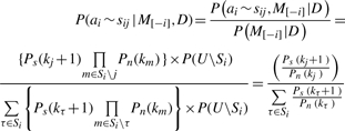(5)

So the normalized likelihood ratio represents the conditional probability for the j-th probable site given the assignment of other tags. Equivalently, this conditional probability serves as our predictive update formula for the Gibbs sampling procedure described below.

In order to calculate likelihood ratios for genomic sites, we need to first map those ambiguous tags to get the number of tags mapped to each specific site. In other words, mapping of ambiguous tags and calculating the likelihood ratios for each site are circular. This circularity led us to adopt Gibbs sampling strategy, which is a stochastic version of EM algorithms, to select reasonable sites for ambiguous tags. To do this, we first initialize the likelihood ratios for genomic sites using the total number of tags that can be probably mapped. Then we map each ambiguous tag to a specific site based on the initial likelihood ratios. To be more specific, we stochastically map each ambiguous tag to a genomic site with the probability equal to the normalized likelihood ratio of the site. Then we update the likelihood ratios given the current mapping of ambiguous tags. We continue the update on the mapping and the calculation of likelihood ratios until there is no significant change. Through the iterative updates (stochastic mapping and parameter updating), the overall likelihood ratios are expected to be optimized, and so we achieve an accurate mapping of ambiguous tags. Since the complete normalized likelihood ratio for a configuration of mapping is proportional to

(6)

where i is the index of genomic sites with tags mapped, we can rewrite this formula based on tag counts and obtain the formula as

(7)

where n(τ) represents the number of sites with τ tags mapped. Here, σ represents the set of tag counts for all sites. For instance, if σ consists of large numbers, it means that most sites are mapped with large number of tags and the mapping is a reasonable one. Otherwise, most sites are mapped with a small number of tags and the set of tags are scattered into diverse sites. Taking the logarithm of this formula and dividing by Z, the total number of tags, we get

(8)

When Z is sufficiently large, it approaches the relative entropy between P_s and P_n on the subset of σ. So essentially, the Gibbs sampling procedure described above searches a certain subset σ to maximize the relative entropy. When σ consists of only large numbers, the relative entropy is larger. This analysis further demonstrates that our algorithmic design is reasonable. Equation (8) shows that by using normalized likelihood ratios, our objective function is equivalent to the relative entropy.

In theory, Gibbs sampling will have good performance given a sufficient number of iterations. Thus, there may be concerns about the time necessary for the algorithm to converge. However, since unique tags count for the majority of the whole set of tags, and these help to guide the mapping of ambiguous tags, this has the effect of shortening the algorithm time significantly. In our experience, about five iterations are sufficient for convergence.

2.3 Algorithm

Next we describe each step of the algorithm in detail along with the definitions of necessary concepts. The scheme of the method is shown in Figure 1.

Phase 1. Initialization

Step 0. The program Bowtie (Langmead et al., 2009) is used to map all sequence tags to the genome and only genomic loci with significant sequence similarities are used for the following steps. Sequence tags are classified into unique tags and ambiguous tags by the Bowtie mapping algorithm.

Step 1. To calculate the likelihood ratios, we need to model the distributions of tag counts for real modified sites (P_s) and for background (P_n). For real modified sites, we use the Normal distribution to approximate the real distribution of tag numbers

(9)

To identify genomic sites that are most likely to actually be modified (i.e. real-modified sites), we use sites with large numbers of mapped unique tags. We then use the numbers of unique tags associated with those sites to calculate the average tag count and standard deviation for each site genome wide. Note that the average tag count calculated here is corrected by a factor which takes into consideration that the real average tag count will be greater once ambiguous tags are included. For background, we use the Poisson distribution to approximate the background distribution of tag counts

(10)

The Poisson distribution is an appropriate model for counting processes that produce rare random events and thus can be applied here to describe the background tag count distribution. We count the total number of tags (both unique and ambiguous tags) and calculate the average tag number for each site. The average tag number serves as the parameter (λ) of Poisson distribution. After getting all the parameters, we calculate the likelihood ratios for various tag counts

(11)

and get a table of likelihood ratios which will be used in subsequent steps.

Step 2. In order to obtain the initial settings of likelihood ratios for all the probable genomic loci, we use the number of tags of each site (both unique and ambiguous tags) to calculate the likelihood ratios. Since the ambiguous tags have not been assigned to a specific genomic site, here we assign each ambiguous tag to all the probable sites to initialize the likelihood ratios. The calculation of likelihood ratios for various tag numbers has already been done in Step 1 and the algorithm only needs to search the table of likelihood ratios. A special notion here is that we introduce the information content factor (0 < f < 1) of ambiguous tags compared to unique tags. Since the nature of uncertainty of ambiguous tags, the information content of ambiguous tags is smaller than unique tags. Thus, the effective number of ambiguous tags (k_e) is corrected by f and the number of tags used to calculate likelihood ratio is:

(12)

where k_u is the number of unique tags and k_a is the number of ambiguous tags. By the user, f can be set based on their confidence of ambiguous tags and provide flexibility of the method. The suggested value of f is the inverse of the mean number of associated sites of ambiguous tags. If the mean number of associated sites of ambiguous tags is larger, then f should be made smaller to weight unique tags more heavily for the mapping.

Phase 2. Iterative weighted mapping

Step 3. Given the likelihood ratio (LR_i) of probable site j (j = 1, 2, …, n_j) for ambiguous tag a_i, the algorithm stochastically selects a probable site and assigns it as the site of the corresponding ambiguous tag. The probability (P_ij) of probable site j to be selected for a_i is proportional to the likelihood ratio of site j.

(13)

where k = 1, 2, …, n_j.

Thus, probable sites with higher likelihood ratios will have a greater chance of being assigned.

Step 4. Based on the current assignments of sites for ambiguous tags obtained from Step 3, the likelihood ratios of all the probable sites are updated. The new likelihood ratio of each probable site is obtained accordingly to the current number of tags assigned to the site.

Step 5. Iterate through Steps 3 and 4 until no significant changes occur, i.e. until convergence. For a given threshold, if the number of reassignments of ambiguous tags is smaller than the threshold, then the iterations will stop and output the final mapping of tags.

3 RESULTS

3.1 Sequence tag datasets

In order to test the performance of our algorithm, we randomly selected ∼50 000 sites of the human genome as a benchmark. Each site is 147 bp in length (i.e. mono-nucleosomal) and the set of sites contains transposable elements and simple repeats in the same fractions as the human genome. Then we generate short sequence tags from these sites under a range of set of parameters. These parameters include sequence tag length (L), signal-to-noise ratio (SNR) and sequencing error level (SE). In theory, shorter sequence tags are expected to have more ambiguous tags. To test the performance of our algorithm on different sequence tag lengths, we generate libraries with 20 bp tags and libraries with 35 bp tags. SNR corresponds to the specificity of the ChIP experiments. Noise here means the fraction of sequence tags derived from sites which are not the real modified sites. In experiments with high specificity, the majority of sequence tags are derived from the real modified sites, while in experiments with high level of noise, there are increased number of sequence tags derived from other sites. And we define the SNR as the ratio of the probability that a sequence tag is derived from the real modified sites over the probability that a sequence tag is derived from other sites. To test our algorithm's performance under different SNRs, we generate libraries with SNR set as 99 (corresponds to 99% tags derived from real modified sites) and libraries with SNR set as 9 (corresponds to 90% tags derived from real modified sites). The sequencing error level corresponds to the probability of errors in high-throughput sequencing. We generate libraries with sequencing error levels as 2/5L and 4/5L. The reason to set SE this way is as follows. We assume that the sequencing errors on different sites are independent from each other. This is not completely true in reality but is acceptable as a first-order approximation. Then the total number of errors for each sequence tag with length L would follow binomial distribution. So under SE = 2/5L, the fraction of sequence tags without errors is ∼60% and under SE = 4/(5L), the fraction is ∼50%. It means that the quality of the simulated sequencing is not very good. Under such conditions, some sequence tags might be mis-mapped or become ambiguous tags. The purpose of this setting is to make sure that our algorithm test results are conservative.

Since each of these three parameters only has two optional values, there are eight combinations of different values of those parameters and so we generate one sequence tag library for each combination of the parameter values. The parameters for each library are listed in Supplementary Table S1.

We also used a second larger benchmark set consisting of 173 877 sites of the human genome. These sites were obtained from a ChIP-seq study of histone modifications based on ABI SOLiD sequencing platform (Victoria V. Lunyak, unpublished data) that only used unique sequence tags, and each site has significant number of tags. This dataset was used because it mimics conditions one would expect for real sites: a larger number of total sites and a realistic distribution of sites along the human genome. In order to test our algorithm, we generated sequence tags for these sites the same way as described above under one set of parameters (Supplementary Table S1).

After preparing sequence tags, we ran the program Bowtie (Langmead et al., 2009) to map the sequence tags to the human genome. The fractions of ambiguous tags in the nine libraries range from 9.7% to 37.6%. The fraction of sites undetected using unique tags alone are influenced by the tag threshold used. Higher threshold cause more undetected sites. For the lowest threshold (four tags) used in our analyses, the fractions of undetected sites range from 16.4% to 28.4%. These values underscore the importance of accurately mapping ambiguous tags to recover undetected sites.

3.2 Fraction of correctly mapped ambiguous tags

The first and most direct measurement of the algorithm performance is the fraction of correctly mapped ambiguous tags. Since the fraction method does not assign the ambiguous tags to a specific site, this measurement is not applicable. So we compared our algorithm against the MAQ software method, which randomly selects a site for each ambiguous tag. The comparison on the eight sequence tag libraries shows that our algorithm correctly maps from 49% to 71% of ambiguous tags, while the MAQ method correctly maps from 8% to 23% of ambiguous tags (Fig. 2). Over all eight sequence tag libraries evaluated, our algorithm maps from 38% to 51% more tags than MAQ. In the best case, our algorithm maps the majority of ambiguous tags (71%) and only a small fraction of information is lost.

Fig. 2.

Fractions of correctly mapped ambiguous tags for each library. Library descriptions are given in Supplementary Table S1. Gray bars show result based on MAQ, and black bars show results based on our Gibbs sampling algorithm.

3.3 Comparison of rescued sites

The other measurement of the algorithm's performance is the numbers and fractions of correctly ‘rescued’ genomic sites, which can not be observed by unique tags alone. An important issue regarding the rescued sites is the tag number threshold, above which a site is called rescued with a certain number of tags (Fig. 3A). Different thresholds will result in different sets of true positives, false positives and false negatives. Since there are various methods to decide the threshold and different users usually set different thresholds, we tested our algorithm's performance on a set of three different thresholds (four, six and eight tags). Together with the previously described the nine sequence tag libraries we use, this results in a set of 27 conditions for analysis.

Fig. 3.

Compariion of algorithm performance. (A) Illustration of data used to test algorithm performance. (B) Variant tag count thresholds could used in the algorithm tests. (C) Recall and precision fractions for map sites are shown for the algorithms compared here (MAQ, blue; fraction method, dark blue; Gibbs sampling method, green) over eight tag libraries. (D) Recall and precision are shown for the larger tag library across three tag thresholds.

The first thing we did was to compare the numbers of genomic sites identified using unique tags alone to the numbers of genomic sites identified by including ambiguous tags with our method (Supplementary Table S2). Over the 27 conditions, the inclusion of ambiguous tags yields an average increase of 11.46% in the fraction of genomic sites accurately identified. The use of ambiguous tags resulted in the identification of 2602–51 508 sites missed with unique tags alone.

Next, we compared our method for including ambiguous tags to the MAQ and fraction methods. To do this, after excluding sites that can be found by unique tags alone, we divide the set of sites rescued by ambiguous tags into two subsets by comparing the set with the benchmark. The correctly rescued sites are true positives (TP) and other sites are false positives (FP). The sites in the benchmark which remain undiscovered are false negatives (FN) (Fig. 3B). In order to test the performances, we employ recall RE = TP/(TP + FN) and precision PE = TP/(TP + FP) as measurements.

For the four libraries with 35 bp tags and the four libraries with 20 bp tags, our algorithm shows the highest recall over all conditions (six-tag threshold shown in Figs. 3C and 4 and eight-tag thresholds shown in Supplementary Fig. S1 and numbers of sites shown in Supplementary Table S3). Our algorithm also has the highest precision for these libraries over 14 of the 24 conditions evaluated (Fig. 3C, Supplementary Fig. S1). For the 10 cases where our algorithm did not show the highest precision, the difference from the fractional method was marginal (Supplementary Table S3). In general, when recall increases precision may be expected to decrease. The simultaneous increase in both recall and precision in 14 cases evaluated here supports the improved performance of our algorithm. To more quantitatively evaluate the improvement in the performance of our algorithm for both recall and precision together, we used the harmonic mean (F) of the recall and precision values for each condition (i.e. each library and threshold combination). The F-values are higher for our algorithm over all conditions, indicating an improvement in performance when recall and precision considered together (Supplementary Table S4). Similar results can be seen when the larger tag library is evaluated with our algorithm over the three thresholds. Recall improves substantially in all cases, and precision decreases marginally for thresholds 6 and 8 (Fig. 3D and Supplementary Table S5). The F-values showing the combined recall and precision performance are higher for our method over all three thresholds (Supplementary Table S4).

Fig. 4.

Examples of ambiguous tag mapping results. Tracks are shown through UCSC Genome Browser. The track of real sites shows the sites in the benchmark libraries. The track of Fraction method shows the mapping result by fraction method and the track of Gibbs method shows the mapping result by our Gibbs method. The heights of data represent the number of tags mapped to those sites. The tracks of repetitive genomic regions (segmental duplications, interspersed repeats and simple repeats) are also shown.

In Figure 4, we provide two examples of our mapping results with the comparison against the benchmark and the result of fraction method. It can be seen that our algorithm rescues more sites than fraction method, and that the average number of tags at rescued sites is higher than seen for the fraction method. This can be attributed to the fact that the fraction method assigns a fraction of ambiguous tags on each site and wastes information on other sites. The greater number of tags per rescued site can help to ensure that these sites are robust to different user thresholds that are employed to distinguish signal from noise.

It should be noted that the two examples shown here represent segmental duplications (Fig. 4A) and satellite regions (Fig. 4B), respectively. It is expected that such highly repetitive regions will produce many ambiguous tags and thus would be difficult to uncover with ChIP-seq. However, our method achieves good performance in such repetitive regions. Furthermore, the second example is located very near to the centromere of chromosome 7. Centromeric regions are important in various cellular processes, such as cell division, and correct mapping of ambiguous tags to centromeric regions could help to uncover specific biological roles for such regions.

3.4 Biological relevance

Transposable elements, simple repeats, micro-satellites, segmental duplications and pericentromeric regions are genomic regions rich in repeat sequences. These regions could produce large numbers of ambiguous tags and will be difficult to uncover due to the technical problem of mapping ambiguous tags. The ability to correctly map ambiguous tags may facilitate novel discoveries regarding the biological significance of such repeat regions, many of which have been ignored in past chromatin immunoprecipitation studies. For instance, we show that our method is able to detect previously uncharacterized segmental duplications and satellite regions in Figure 4. In addition, our method uncovered a previously undetected modified histone site in the proximal promoter region of the CWF19-like one cell cycle control protein.

To further investigate whether our algorithm really helps us to find more sites in genomic repeats, we used the UCSC genome browser (Karolchik et al., 2004; Kent et al., 2002) to count the numbers and fractions of rescued sites in those regions and compared them against using unique tags alone (Fig. 5). This analysis demonstrates that our algorithm is able to rescue substantial numbers of sites in genomic repeat regions, especially for segmental duplications and pericentromeric regions. Unique tags can only uncover around half of the sites in segmental duplications and pericentromeric regions, while our algorithm could uncover the majority of those sites (Fig. 5B). It is evident that our method has the potential to generate additional biological knowledge from ChIP-seq experiments.

Fig. 5.

(A) The number of correctly discovered sites in various genomic features by unique tags alone (white) and our Gibbs method (black) compared with the corresponding numbers in the benchmark library. (B) The fractions of correctly discovered sites in various genomic features by unique tag alone (white) and our Gibbs method (Black). [TE, transposable element; s_r, simple repeats; microSat, microsatellites; seg_dup, segmental duplication; centro, peri-centromeric region].

4 DISCUSSION

Based on the results described above, we have shown that our algorithm significantly improves the accuracy of mapping ambiguous tags. The essential information used by the algorithm is the association between co-located sequence tags, which was originally utilized by Faulkner et al. (2008) in the fraction method. Our contribution to this class of approach is to employ iterative probabilistic methods to achieve better performance. The use of likelihood ratios not only reflects the information on sequence tag associations, but also the background distribution information. Furthermore, likelihood ratios are not linear to tag counts, but increase sharply for large tag counts and thus efficiently avoid wasting signal on sites with small tag counts. The Gibbs sampling procedure enables us to sample in the space of mapping and achieve a reasonable assignment of sites to sequence tags. For most experiments, unique tags are the majority of tags and they can guide the sampling efficiently. Thus, Gibbs sampling does not require too much time to reach the final result. We have also shown that correct mapping of ambiguous tags can facilitate our understanding of biology by recovering repeated genomic sites which are prone to produce ambiguous tags.

Although the length of sequence tags is increasing, there will still be a certain amount of ambiguous tags. As shown in Figure 4, genomic sites, such as segmental duplications and microsatellites will always produce ambiguous tags by their nature: with multiple copies in the genome. So the task of mapping ambiguous tags will not disappear due to the experimental technique advancements in short term, and our algorithm provides an efficient way to solve this problem.

Funding: Bioinformatics Program at the Georgia Institute of Technology (to J.W.); Alfred P Sloan Research Fellowship in Computational and Evolutionary Molecular Biology (BR-4839, to I.K.J. and graduate student A.H.); National Institutes of Health pilot projects (UL1 DE019608 to V.V.L.); Buck Institute Trust Fund (to V.V.L.).

Conflict of Interest: none declared.

REFERENCES

- Barski A, et al. High-resolution profiling of histone methylations in the human genome. Cell. 2007;129:823–837. doi: 10.1016/j.cell.2007.05.009. [DOI] [PubMed] [Google Scholar]
- Bock C, Lengauer T. Computational epigenetics. Bioinformatics. 2008;24:1–10. doi: 10.1093/bioinformatics/btm546. [DOI] [PubMed] [Google Scholar]
- Faulkner GJ, et al. A rescue strategy for multimapping short sequence tags refines surveys of transcriptional activity by CAGE. Genomics. 2008;91:281–288. doi: 10.1016/j.ygeno.2007.11.003. [DOI] [PubMed] [Google Scholar]
- Feschotte C. Transposable elements and the evolution of regulatory networks. Nat. Rev. Genet. 2008;9:397–405. doi: 10.1038/nrg2337. [DOI] [PMC free article] [PubMed] [Google Scholar]
- Hashimoto T, et al. Probabilistic resolution of multi-mapping reads in massively parallel sequencing data using MuMRescueLite. Bioinformatics. 2009;25:2613–2614. doi: 10.1093/bioinformatics/btp438. [DOI] [PubMed] [Google Scholar]
- Karolchik D, et al. The UCSC Table Browser data retrieval tool. Nucleic Acids Res. 2004;32:D493–D496. doi: 10.1093/nar/gkh103. [DOI] [PMC free article] [PubMed] [Google Scholar]
- Kent WJ, et al. The human genome browser at UCSC. Genome Res. 2002;12:996–1006. doi: 10.1101/gr.229102. [DOI] [PMC free article] [PubMed] [Google Scholar]
- Langmead B, et al. Ultrafast and memory-efficient alignment of short DNA sequences to the human genome. Genome Biol. 2009;10:R25. doi: 10.1186/gb-2009-10-3-r25. [DOI] [PMC free article] [PubMed] [Google Scholar]
- Lawrence CE, et al. Detecting subtle sequence signals: a Gibbs sampling strategy for multiple alignment. Science. 1993;262:208–214. doi: 10.1126/science.8211139. [DOI] [PubMed] [Google Scholar]
- Li H, et al. Mapping short DNA sequencing reads and calling variants using mapping quality scores. Genome Res. 2008;18:1851–1858. doi: 10.1101/gr.078212.108. [DOI] [PMC free article] [PubMed] [Google Scholar]
- Neuwald AF, et al. Gibbs motif sampling: detection of bacterial outer membrane protein repeats. Protein Sci. 1995;4:1618–1632. doi: 10.1002/pro.5560040820. [DOI] [PMC free article] [PubMed] [Google Scholar]
- Park PJ. ChIP-seq: advantages and challenges of a maturing technology. Nat. Rev. Genet. 2009;10:669–680. doi: 10.1038/nrg2641. [DOI] [PMC free article] [PubMed] [Google Scholar]
- Thurman RE, et al. Identification of higher-order functional domains in the human ENCODE regions. Genome Res. 2007;17:917–927. doi: 10.1101/gr.6081407. [DOI] [PMC free article] [PubMed] [Google Scholar]
- Zhang Y, et al. Model-based analysis of ChIP-Seq (MACS) Genome Biol. 2008;9:R137. doi: 10.1186/gb-2008-9-9-r137. [DOI] [PMC free article] [PubMed] [Google Scholar]
Associated Data
This section collects any data citations, data availability statements, or supplementary materials included in this article.