

Abstract
Motivation: The rapid development of next-generation sequencing technologies able to produce huge amounts of sequence data is leading to a wide range of new applications. This triggers the need for fast and accurate alignment software. Common techniques often restrict indels in the alignment to improve speed, whereas more flexible aligners are too slow for large-scale applications. Moreover, many current aligners are becoming inefficient as generated reads grow ever larger. Our goal with our new aligner GASSST (Global Alignment Short Sequence Search Tool) is thus 2-fold—achieving high performance with no restrictions on the number of indels with a design that is still effective on long reads.
Results: We propose a new efficient filtering step that discards most alignments coming from the seed phase before they are checked by the costly dynamic programming algorithm. We use a carefully designed series of filters of increasing complexity and efficiency to quickly eliminate most candidate alignments in a wide range of configurations. The main filter uses a precomputed table containing the alignment score of short four base words aligned against each other. This table is reused several times by a new algorithm designed to approximate the score of the full dynamic programming algorithm. We compare the performance of GASSST against BWA, BFAST, SSAHA2 and PASS. We found that GASSST achieves high sensitivity in a wide range of configurations and faster overall execution time than other state-of-the-art aligners.
Availability: GASSST is distributed under the CeCILL software license at http://www.irisa.fr/symbiose/projects/gassst/
Contact: guillaume.rizk@irisa.fr; dominique.lavenier@irisa.fr
Supplementary information: Supplementary data are available at Bioinformatics online.
1 INTRODUCTION
Next-generation sequencing (NGS) technologies are now able to produce large quantities of genomic data. They are used for a wide range of applications, including genome resequencing or polymorphism discovery. A very large amount of short sequences are generated by these new technologies. For example, the Illumina-Solexa system can produce over 50 million 32–100 bp reads in a single run. A first step is generally to map these short reads over a reference genome. To enable efficient, fast and accurate mapping, new alignment programs have been recently developed. Their main goals are to globally align short sequences to local regions of complete genomes in a very short time. Furthermore, to increase sensitivity, a few alignment errors are permitted.
The seed and extend technique is mostly used for this purpose. The underlying idea is that significant alignments include regions having exact matches between two sequences. For example, any 50 bp read alignments with up to three errors contains at least 12 identical consecutive bases. Thus, using the seed and extend technique, only sequences sharing common kmers are considered for a possible alignment. Detection of common kmers is usually performed through indexes localizing all kmers.
Recently, several index methods have been investigated and implemented in various bioinformatics search tools. The first method, used by SHRiMP (Rumble et al., 2009) and MAQ (Li,H. et al., 2008), creates an index from the reads and scans the genome. The advantage is a rather small memory footprint. The second method makes the opposite choice: it creates an index from the genome, and then aligns each read iteratively. PASS (Campagna et al., 2009), SOAPv1 (Li,R. et al., 2008), BFAST (Homer et al., 2009) and our new aligner GASSST (Global Alignment Short Sequence Search Tool); use this approach. The last method, used in CloudBurst, indexes both the genome and the reads. Although more memory is needed, the algorithm exhibits better performance due to memory cache locality. Another short read alignment technique, used in Bowtie (Langmead et al., 2009), SOAPv2 (Li et al., 2009) and BWA (Li and Durbin, 2009), uses a method called backward search (Ferragina and Manzini, 2000) to search an index based on the Burrows–Wheeler transform (BWT; Burrows and Wheeler, 1994). Basically, it allows exact matches to be found before using a backtracking procedure that allows the addition of some errors. Although this technique reports extremely fast running times and small memory footprints, some data configurations lead to poor performances. (http://bowtie-bio.sourceforge.net/manual.shtml).
Moreover, in order to speed-up computations, some methods restrict the type or the number of errors per alignment to a few mismatch and indel errors. In the building alignment process, computing the number of mismatches requires linear time, whereas indel errors require more costly algorithms such as the dynamic programming techniques used in the Smith–Waterman (Smith and Waterman, 1981) or Needleman–Wunsch (NW; Needleman and Wunsch, 1970) algorithms. For instance, MAQ, Eland and Bowtie do not allow gaps. EMBF (Wendi et al., 2009), SOAPv1 and SOAPv2 allow only one continuous gap, while PASS, SHRiMP, BFAST and SeqMap (Jiang and Wong, 2008) allow any combination of mismatch and indel errors. GASSST, as well, considers any combination of mismatch, insertion or deletion errors. In most applications, when reads are very short, dealing with a restricted number of errors is acceptable. On the other hand, when longer reads are processed, or when more distant reference genomes are compared, this restriction may greatly affect the quality of the search.
In this article, we introduce GASSST, a new short read aligner for mapping reads with mismatch and indel errors at a very high speed. We show how a series of carefully designed filters allows false positive positions to be quickly discarded before the refinement extension step. In particular, GASSST is compared with similar state-of-the-art programs: BFAST, BWA, PASS and SSAHA2.
2 APPROACH
GASSST uses the seed and extend strategy and indexes the genome. The seed step provides all potentially homologous areas in the genome with a given query sequence. The traditional way to accomplish this step is through a hash-table of kmers for selecting regions sharing common kmers with query sequences. To include gaps, the extend step is carried out with a dynamic programming algorithm (NW). This approach provides a high degree of accuracy, but is prohibitively expensive due to the high number of costly NW extensions that must be performed.
To tackle this issue, several approaches have been proposed. The SHRiMP implementation (Rumble et al., 2009) provides an improved seed step with spaced seeds and Q-gram filters to restrict the size of the candidate hit space. Then, a carefully optimized vectorized Smith–Waterman extension is run to perform the extend step. BFAST (Homer et al., 2009) uses long spaced seeds to limit the amount of candidate locations, yet still achieves high sensitivity through the use of multiple indexes. PASS (Campagna et al., 2009) implements another solution: a filter is introduced before the full extend step to rule out areas that have too many differences with the query sequence. A precomputed table of all possible short words, aligned against each other, is built to perform a quick analysis of the flanking regions adjacent to seed words.
The GASSST strategy is similar: a traditional anchoring method is used followed by a NW extension step. However, fast computation is achieved thanks to a very efficient filtering step. Candidate positions are selected through a new carefully designed series of filters of increasing complexity and efficiency. Two main types of filter are used. One is related to the computation of an Euler distance between nucleotide frequency vectors as defined by Wendi et al. (2009). The idea is this: if one sequence has, for example, three more ‘T’ nucleotides than another, then the alignment will have at least three errors (mismatches or indels).
The other includes precomputed tables, as in PASS, to produce a score based on the NW algorithm, but brings the strategy to a higher level; instead of addressing large tables, as PASS does, we designed an algorithm able to reuse small tables along the whole query sequence. In this way, the filter is much more selective and discards a very large number of false positives, thus drastically decreasing the time spent in the final extend step.
GASSST's originality comes then from the use of a small lookup table. More precisely, the precomputed alignment scores of all possible pairs of words of length w can be stored in a memory of size 42w bytes, if a score is memorized in a single byte. For PASS, the size of the lookup table is 414 = 256 MB. This fits into any computer's main memory, but not in the first-level CPU cache. Hence, random accessing of the table, even if it avoids many computations, may still be costly. On the contrary, the GASSST algorithm manipulates a small table of 64 KB which easily fits into the cache memory, providing fast filtering compared with non-precomputed calculations.
3 METHODS
GASSST algorithm has three stages: (i) searching for exact matching seeds between the reference genome and the query sequences; (ii) quickly eliminating hits that have more than a user-specified number of errors; and (iii) computing the full gapped alignment with the NW algorithm. These three steps are referred to, respectively, as seed-filter-extend. The novelty of the GASSST approach relies on a new highly efficient filter method.
3.1 Seed
GASSST creates an index of all possible kmers in the reference sequence and then scans every query sequence to find matching seeds. When seeds longer than 14 are selected the algorithm uses a simple hash-table mechanism. For each seed position in the reference sequence, the index contains the sequence number, the position where it occurs and the flanking regions (binary encoded). Up to 16 nt are stored on the left and on the right of the seed in order to speed-up the next filtering steps. The size of the index is equal to 16 × N bytes, with N the size of the reference sequence. If large reference sequences which exceed the memory size are considered, a simple partitioning scheme is provided; the reference sequence is split into as many parts as necessary to fit in the available RAM. Each part is then processed iteratively.
3.2 Tiled-NW filter
A lookup table, called pre-computed score table PSTl, containing all the NW alignment scores of all possible pairs of l nt long words is first computed. PASS uses a PST7 to analyze discrepancies near the 7 nt long flanking region adjacent to the seeds. The bigger the table, the better the filtering. But unfortunately, the table grows exponentially with l. To address this issue, GASSST analyzes discrepancies in a region of any length thanks to the reuse of a small PST4 table. The goal is to provide a lower bound approximation of the real NW score along the whole alignment. If estimated lower bounds are greater than the maximum number of allowed errors, then alignments are eliminated. If not, alignments are passed to the next step.
The following values are used for the NW score computation: 0 for a match, and 1 for mismatch and indel errors. Consequently, the final score indicates the number of discrepancies in the alignment.
In the following, only the right side of the seed is considered, the other side being symmetrical.
Definition 1. —
We call TNWl(n) the score of a region of n nucleotides which are adjacent to the right of the seed and which are computed with a PSTl. TNW stands for Tiled NW. TNWl(full) operates on the maximum length available, i.e. from the right of the seed to the end of the query sequence.
Definition 2. —
If S1 and S2 are the two sequences directly adjacent to the right of the seed, we call PSTl(i, j) the pre-computed NW score for the two l nt long words S1(i, i + l − 1) and S2(j, j + l − 1).
If Gm is the maximum number of allowed gaps, TNWl(n) is computed with the following recursion:
If n ≤ l then
| (1) |
Else
| (2) |
With
Figure 1B shows a graphical representation of this recursion.
Fig. 1.

Computation of a semi-global alignment (only the query sequence needs to be globally aligned), in the case of a maximum of 1 error. (A) Dynamic Programming. With 12 nt long sequences and a traditional dynamic programming algorithm, cell calculations can be limited in a band, but there are still 34 cells to compute. (B) Tiled Algorithm. With a precomputed table score of size 4 × 4, the tiled algorithm is performed in only three steps. The first step requires one table access, while the second and third steps both require three table accesses. Here, the score given by the tiled algorithm is the same as the full dynamic programming algorithm—there are two errors in the alignment. In the general case, the tiled algorithm only gives a lower bound of the number of errors present in the alignment.
Complexity of the filter. GASSST uses a PST4 lookup table. By storing each score in a single byte, its size is equal to 64 KB. This small size allows the PST4 to fit in a CPU cache of today's desktop computers. But if TNW4(4) requires a few clock cycles to be accessed, its filtering power is limited.
In the general case, the number of PSTl accesses Nacc[TNW(n)] needed for the computation is in 𝒪(n). If Gm is the maximum number of allowed gaps, the exact formula is:
| (3) |
The filter works with iterative l-sized levels. The first one takes one access, then each following level requires (1 + 2 · Gm) PSTl accesses. Each new level filters more and more false positive alignments. Large PSTl tables lead to fewer levels and better accuracy, but they imply longer execution times since the number of memory cache misses increases rapidly with bigger tables.
3.3 Frequency vector filter
The frequency vector filter of GASSST is the same as the one used in EMBF (Wendi et al., 2009). The idea is quite simple: if one sequence has, for example, three more ‘G’ nucleotides than another sequence, then their alignment will have at least three errors. If the user-specified maximum number of errors is 2, then the alignment can be directly eliminated.
For a sequence S = s1s2…n of characters in the alphabet Σ = {a1, a2,…, ap}, the frequency vector F = {f1, f2,…, fm} is defined as:
| (4) |
With
| (5) |
The Euler distance has to be computed on similar frequency vectors, i.e. referring to sequences of equal length. The distance is computed with:
| (6) |
In GASSST, frequency vectors of sequences of up to 16 nt on both sides of the seed are computed. Actually, this value is often limited by the length of the reads, and forbids vectors of the reference sequence to be computed at runtime. Indeed, the size of subsequences depends on the size available on the read, which is often less than 16 and which is only known at compute time. The Euler distance is computed between the frequency vectors of the read and the genome. If the result is greater than the maximum number of errors then the alignment is discarded.
The computation of the frequency vectors is vectorized and quickly performed thanks to the binary format of the seed flanking regions. The frequency vectors and the Euler distance computations are both vectorized to benefit from vector execution units present in modern processors. Since a 16 nt sequence is 32-bit encoded, counting the frequency of a single nucleotide can be done with bit-level logical operations that operate on traditional 32-bit words. The vectorization consists of simultaneously computing values for the four nucleotides of the alphabet and operates on 128-bit wide words. The frequency distance vectorized filter is referred to as FD-vec.
3.4 Filters combination
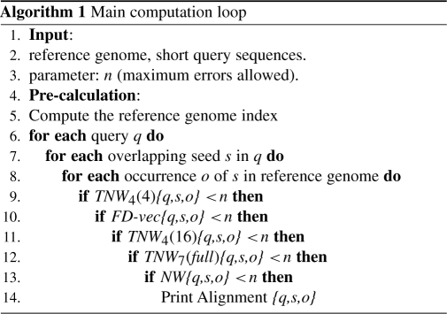
The goal of the filter step is to eliminate as many false positive alignments generated by the seed step as possible, and in the fastest possible way. This is done by ordering the individual filters from the fastest to the most complex and powerful. Algorithm 1 shows the main computation loop of GASSST with the series of filters. TNW4(4) is first since it is the fastest. It is followed by the vectorized frequency filter that rules out remaining false positive alignments. Then a more thorough filter is used (TNW4(16)). The last filter is a TNW7(full) filter which is applied on the full length of the sequence and with a PST7 in order to eliminate a maximum number of false positive alignments. It is computationally intensive, but it comes at the end when most alignments have already been ruled out.
Finally, the true NW alignment is computed on alignments that go through all filters. This combination of filters ensures an efficient and fast filtering in a wide range of configurations, from short to longer reads, with low or high polymorphism.
One important point is that these filters only discard alignments which are proven to have too many errors and that would have been eliminated by the NW algorithm. They never eliminate good alignments, hence they do not decrease sensitivity.
Moreover, to reduce running time, the search is stopped when a maximal number of occurrences of a seed in the reference sequence has been reached. This kind of limitation is present in most other aligners. The only difference here is that a threshold is also checked in some stage of the filtering process. The threshold is automatically computed according to seed length and reference sequence size. Users can control the speed/sensitivity trade-off of this heuristic through a parameter s in 0–5 which modulates this threshold.
3.5 Extend
The extend step receives alignments that passed the filter step. It is computed using a traditional banded NW algorithm. Significant alignments are then printed with their full description. It should be noted that if the filter step provides good efficiency, no optimization of the extend step is required. Indeed, if most false positive alignments have already been ruled out, the extend step should only take a negligible fraction of the total execution time.
4 RESULTS
4.1 Implementation
GASSST is implemented in C++ and runs on Linux, OS X and Windows. It benefits from vector execution units with the use of SSE (streaming SIMD extensions) instructions, and is multi-threaded. It performs accurate and fast gapped alignments and allows the user to specify the number of hits given per read (option -h). A tool is provided to convert GASSST results to SAM format and compute GASSST mapping quality. GASSST is distributed under the CeCILL software license (http://www.cecill.info). Documentations and source code are freely available from the following web site: http://www.irisa.fr/symbiose/projects/gassst/.
4.2 Evaluated programs
The performance of GASSST is compared with four other programs: PASS 0.74 (Campagna et al., 2009) BFAST 0.6.3c (Homer et al., 2009), BWA 0.5.7 (Li and Durbin, 2009) and SSAHA 2.5.2 (Ning et al., 2001) . PASS indexes the genome and scans reads. It uses a precomputed NW table to filter alignments before conducting the extension with a dynamic programming algorithm. BFAST is currently one of the most popular tools. It relies on large spaced seeds for a fast execution, and on many different indexes for sensitivity.
BWA uses another approach, based on the BWT, and is probably one of the fastest aligners to date for alignments with a low error rate. We also tested the BWA-SW variant intended to work best for longer reads. In the following, ‘BWA’ refers to the BWA short read mode and ‘BWA-SW’ to the long read variant.
The computer used for the tests is an Intel Xeon E5462 with 32 GB RAM running at 2.8 GHz. Although all programs tested are able to benefit from multi-threaded computations, we choose to compare performance on a single thread, as it is enough to assess their respective strong or weak points.
We ran experiments with real datasets to give an indicative behavior. Detailed program analysis was conducted on simulated data where alignment correctness could be assessed.
4.3 Evaluation on real data
Performance was evaluated on three real datasets of short reads obtained from the NCBI Short Reads Trace Archive. The three sets contain, respectively, 11.9 million sequences of 36 bases, 6.8 million sequences of 50 bases and 8.5 million sequences of 76 bases of accession numbers SRR002320, SRR039633 and SRR017179. They are all aligned with the whole human genome.
BWA short read aligner was run with default options, BFAST was run with its 10 recommended indexes and default options, GASSST and PASS were set to search for alignments with at most 10% errors. We measured the execution time and the percentage of mapped reads having a mappinq quality greater than or equal to 20. The results are presented in Table 1.
Table 1.
Evaluation on real data
| Read | Software | Index (s) | Align (s) | Q20% | Q20 |
|---|---|---|---|---|---|
| length | Error rate (%) | ||||
| 36 bp | GASSST | 1712 | 3211 | 34.5 | 0.14 |
| BFAST | 520 800 | 17 520 | 41.8 | 0.12 | |
| BWA | 5158 | 3739 | 35.4 | 0.17 | |
| PASS | 2312 | 5072 | 41.4a | – | |
| 50 bp | GASSST | 1719 | 4090 | 73.7 | 0.04 |
| BFAST | 520 800 | 22 799 | 80.4 | 0.10 | |
| BWA | 5158 | 3043 | 74.5 | 0.17 | |
| PASS | 2144 | 5384 | 79.3a | – | |
| 76 bp | GASSST | 1701 | 8483 | 81.3 | 0.04 |
| BFAST | 520 800 | 161 220 | 85.4 | 0.28 | |
| BWA | 5158 | 3101 | 86.4 | 0.53 | |
| PASS | 1951 | 118 541 | 87.7a | – |
Datasets consisted, respectively, of 11.9, 6.8 and 8.5 millions of reads of size 36, 50 and 76 bp, of accession numbers SRR002320, SRR039633 and SRR017179. The three datasets were aligned with the whole human genome. The time required to compute the genome index is shown in column 3. For BFAST and BWA, the index was computed only once and stored on disk. Column 4 shows the time required in seconds to align reads, running on a single core of a 2.8 GHz Xeon E4562. Column 5 shows the percentage of reads with a mapping quality greater than or equal to 20 (Q20). Last column is the percentage of Q20 alignments that are probably wrong given the results of other aligners: if a program gives a high mapping quality to a read and another program finds a different alignment of similar alignment score for that read, then the first program is probably wrong.
aSince PASS does not compute mapping qualities, fifth column shows for PASS the percentage of reads with a unique best alignment, and error rate is not computed.
Evaluation on real data is difficult since true alignment locations are unknown. However, it is possible to compare results of different aligners to estimate accuracy, as it is done by Li and Durbin (2010) for their evaluation of BWA-SW. If an aligner A gives a high mapping quality to a read and another aligner B finds an alignment at another position for that same read with an alignment score better or just slightly worse, then A alignment is probably wrong. A score for each read is computed as the number of matches minus three multiplied by the number of differences (mismatches and gaps). We say that A alignment is questionable if the score derived from A minus the score derived from B is less than 20. Since this evaluation method is approximate, a full evaluation was conducted on simulated data in Section 4.5.
On short 36 bp reads, GASSST performance is comparable to BWA. On longer 76 bp reads both PASS anf BFAST becomes very slow. On the other hand, the GASSST combination of filters still works well for the 76 bp dataset.
GASSST and PASS currently cannot store the index on disk, yet index computation time is amortized when working on very large sets of reads. BFAST index time is very long because it uses 10 different indexes, however they are computed only once.
4.4 Filter behavior analysis
We measured the filtering power of the filter combination on the same three datasets of the previous section to validate their efficiency on different configurations. The allowed similarity rate was set to 90% minimum so the number of allowed errors was 3, 4 and 7, respectively. Other program options are possible and would result in different behavior, so the results presented here cannot be generalized and are only intended to provide an indicative example.
Hits coming from the seed step are pipelined through the filters. At each filter step, we calculate the filtering percentage of the individual step as well as the cumulative percentage of hits filtered so far. The NW alignment is seen as the last filter and its result is also included. Table 2 shows the results. The first thing that can be noted is that in all cases the percentage of hits arriving at the NW step is limited to 0.2% of the number of hits generated by the seed phase. This means that without filters, this step would take at least 500 times longer.
Table 2.
Filtering rate on three datasets
| Data Set | Filter Step | Step filter (%) | Total filter (%) |
|---|---|---|---|
| 36 bp | TNW4(4) | 64.9 | 64.9 |
| FD − vec | 72.8 | 90.5 | |
| TNW4(16) | 96.6 | 99.7 | |
| TNW7(full) | 45.9 | 99.8 | |
| NW | 63.8 | 99.9 | |
| 50 bp | TNW4(4) | 41.7 | 41.7 |
| FD − vec | 80.4 | 88.6 | |
| TNW4(16) | 97.5 | 99.7 | |
| TNW7(full) | 88.5 | 99.97 | |
| NW | 67.5 | 99.99 | |
| 76 bp | TNW4(4) | 0.1 | 0.1 |
| FD − vec | 49.8 | 49.9 | |
| TNW4(16) | 93.7 | 96.8 | |
| TNW7(full) | 94.8 | 99.8 | |
| NW | 70.2 | 99.95 |
The first column gives the percentage of hits filtered by a given filter. The second column gives the total percentage of hits filtered by the sequence of filters. Reads were aligned with 10% errors maximum, which means a maximum of 3, 4 and 7 errors, gaps or mismatches, respectively.
Second, one interesting thing to observe is the number of false positive alignments that passed the filters and still arrive at the NW step. The NW step filters about two-thirds of incoming hits, meaning that previous filters have efficiently ruled out most false positive alignments—one alignment out of three that enters the NW step is valid. As expected, on the last dataset (seven allowed errors), the TNW4(4) filter efficiency is very poor since it can only manage a maximum of four errors on each side of the seed. In the current implementation, this filter is deactivated when the number of errors exceeds 7.
To complete this analysis, we measured the total time spent inside each filter. The program was profiled for a typical execution with the 50 bp dataset. For each step, both the computation time of a single hit in nanoseconds and the total execution time of the step in percentage of the total time of the program were measured. The results are shown in Table 3. The General Overhead mostly represents the cost of line 8 of Algorithm 1, which iterates through hits and loads the associated information. The TNW4(4) filter takes only 5.8 ns, which represents, as expected, only a few clock cycles of the processor. We can also verify that the filters are indeed ordered from the most simple to the most complex. The NW step takes only 3% of the total time, which validates the assessment formulated in Section 3.5 that we do not need to be concerned about its optimization.
Table 3.
Filters execution time
| Step | Execution time | Total percent time |
|---|---|---|
| for one hit (ns) | spent in this step | |
| General Overhead | 13.9 | 33 |
| TNW4(4) | 5.8 | 14 |
| FD − vec | 22.4 | 32 |
| TNW4(16) | 78.5 | 15 |
| TNW7(full) | 356.7 | 3 |
| NW | 4486.5 | 3 |
Average time taken by each filter step for one hit of a 50 bp query, in nanoseconds. Note that only the times of TNW7(full) and NW actually depends on query size since the others only work on a bounded size subsequence.
4.5 Evaluation on simulated data
We simulated 12 datasets containing one million reads each from the entire human genome, with lengths of 50, 100, 200 and 500 bp and with error rates of 2, 5 and 10%. The error rate is the probability of each base being an error, 20% of errors are indel errors with indel length l drawn from a geometric distribution of density 0.7 × 0.3l−1. BFAST is run with options −K 8 and −M 1280 with 10 indexes. GASSST was tested in two different configurations, a fast one with option −s0 and an accurate one with −s3, which controls the speed/sensitivity trade-off of the algorithm by setting a maximum number of occurrences per seed. It is roughly the equivalent of options −K and −M of BFAST. Other GASSST options such as seed length and maximum number of allowed errors were tuned accordingly to the different datasets. BWA and PASS options were also tuned to allow more mismatches and gaps when necessary, and BWA-SW was run with default configuration. Finding the most efficient set of options for each program and each dataset is a lengthy process, so although we did our best to tune options and provide a fair evaluation, in some cases different options may yield better performance. The results are presented in Table 4. Supplementary Table S1 gives the list of options parameters used.
Table 4.
Evaluation on simulated data
| Program | Mode | Metrics | 50 bp |
100 bp |
200 bp |
500 bp |
||||||||
|---|---|---|---|---|---|---|---|---|---|---|---|---|---|---|
| 2% | 5% | 10% | 2% | 5% | 10% | 2% | 5% | 10% | 2% | 5% | 10% | |||
| GASSST | fast | Align sec | 584 | 781 | 1720 | 794 | 981 | 1160 | 2030 | 2314 | 3051 | 6573 | 8453 | 11 859 |
| Sensitivity% | 45.8 | 42.8 | 36.1 | 54.2 | 53.3 | 44.9 | 58.6 | 56.3 | 53.8 | 61.0 | 59.8 | 58.8 | ||
| Accuracy% | 99.2 | 98.5 | 93.8 | 90.5 | 89.4 | 86.9 | 91.9 | 91.5 | 89.7 | 93.0 | 92.8 | 91.7 | ||
| GASSST | accurate | Align sec | 1709 | 2741 | 4706 | 1290 | 1887 | 3262 | 3452 | 6173 | 8744 | 12 864 | 18 737 | 34 222 |
| Sensitivity% | 46.7 | 44.6 | 37.5 | 51.0 | 50.3 | 43.5 | 53.4 | 52.8 | 51.7 | 57.5 | 55.7 | 55.5 | ||
| Accuracy% | 99.8 | 99.3 | 93.5 | 99.7 | 99.4 | 97.5 | 99.9 | 99.8 | 99.3 | 99.9 | 99.9 | 99.7 | ||
| BFAST | Align sec | 2279 | 2044 | 1756 | 15 263 | 15 787 | 11 452 | – | – | – | – | – | – | |
| Sensitivity% | 46.5 | 43.0 | 32.1 | 52.7 | 51.0 | 48.5 | – | – | – | – | – | – | ||
| Accuracy% | 98.8 | 96.1 | 85.2 | 99.0 | 98.7 | 95.8 | – | – | – | – | – | – | ||
| BWA | Align sec | 792 | 1392 | 1572 | 1862 | 4941 | 3364 | 4660 | 2145 | 185 | – | – | – | |
| Sensitivity% | 48.2 | 38.6 | 16.8 | 54.8 | 41.0 | 7.3 | 53.3 | 11.9 | 0.1 | – | – | – | ||
| Accuracy% | 99.2 | 97.4 | 93.5 | 99.7 | 99.0 | 97.9 | 99.8 | 99.6 | 96.7 | – | – | – | ||
| BWA-SW | Align sec | – | – | – | – | – | – | 4699 | 3546 | 2365 | 13 027 | 9646 | 7835 | |
| Sensitivity% | – | – | – | – | – | – | 54.9 | 50.3 | 25.2 | 57.3 | 56.1 | 45.4 | ||
| Accuracy% | – | – | – | – | – | – | 99.4 | 96.9 | 85.7 | 99.2 | 96.8 | 85.2 | ||
| SSAHA2 | Align sec | – | – | – | 27 740 | 41 978 | 45 295 | 22 285 | 27 504 | 65 420 | 179 095 | 415 252 | 275 622 | |
| Sensitivity% | – | – | – | 45.3 | 43.5 | 38.6 | 53.2 | 51.4 | 48.4 | 59.5 | 58.8 | 55.8 | ||
| Accuracy% | – | – | – | 99.8 | 99.1 | 95.3 | 99.8 | 99.1 | 96.0 | 99.8 | 99.2 | 95.3 | ||
| PASS | Align sec | 2012 | 2281 | 5085 | 14 387 | 26 033 | 30 022 | 103 338 | 139 436 | 180 943 | – | – | – | |
| Sensitivity% | 50.0 | 43.8 | 31.3 | 51.6 | 37.5 | 16.4 | 49.3 | 16.6 | 2.8 | – | – | – | ||
| Accuracy% | 96.6 | 93.2 | 82.4 | 98.5 | 94.0 | 86.8 | 97.2 | 93.6 | 92.4 | – | – | – | ||
Data sets containing one million reads each are simulated from the human genome with different lengths and error rate. Twenty percent of errors are indel errors with indel length l drawn from a geometric distribution of density 0.7 · 0.3l−1. The alignment time in seconds only includes the fraction of the total time proportional to the number of reads, i.e, not the time spent in computing or loading the index of the human genome, running on a single core of a 2.8 GHz Xeon E4562 . Computed alignment coordinates are compared to the true simulated coordinates to find sensitivity and accuracy. Sensitivity is the percentage of reads correctly mapped, while accuracy is the percentage of mapped reads that are correctly mapped. A read is considered mapped if it has a unique best alignment. A mapped read is considered correct if it is within 10 bp of its true coordinates. We filtered alignments having a mapping quality less than 20, except for PASS, which does not give mapping quality.
For each run, we reported accuracy, sensitivity and running time. A read is considered to be mapped if it has a unique best alignment. A mapped read is considered correct if it is within 10 bases of the true location. We filtered all alignments that had a mapping quality less than 20, except for PASS which does not compute mapping quality. Sensitivity and accuracy are then, respectively, defined as the percentage of total or mapped reads that are correct. The running time reported does not include index loading or computing phase. Although this choice penalizes BWA, which is the only one not spending noticeable time recomputing or reloading indexes, it is relevant since time spent for the index of the genome is constant and is amortized when dealing with a very large number of reads.
Tests were also conducted with SHRiMP 1.3.1 but not included here since running times were tens to hundreds of times larger than GASSST, rendering evaluation impractical. This corresponds to observations in other studies that had to extrapolate SHRiMP running time (Homer et al., 2009).
For datasets with a low 2% error rate, GASSST performance is comparable with BWA. For example, on short 50 bp reads, GASSST in fast mode obtained 45.8%/99.2% sensitivity/accuracy in 584 s compared with 48.2%/99.2% in 792 s for BWA. For higher error rates, GASSST becomes better than BWA, for example, on the 100 bp reads with 10% error rate GASSST obtained 43.5%/97.5% sensitivity/accuracy in 3262 s compared with 7.3%/97.9% in 3364 s for BWA.
On datasets simulated with a high 10% error rate, GASSST consistently reports better results than other aligners. On the 200 bp 10% dataset, GASSST was the only one able to provide high sensitivity and accuracy within a reasonable amount of time. On the 500 bp dataset, experiments are only conducted on GASSST, BWA-SW and SSAHA2 since other aligners are not designed for this read length. They show that GASSST still performs very well. For example, on the 2% error rate dataset, GASSST obtained results comparable to BWA-SW. With 10% error rate GASSST is eight times faster than SSAHA2 for similar results, whereas BWA-SW accuracy is dropping. BFAST is efficient on short 50 bp reads only, its execution time increases a lot for longer reads.
Overall, these experiments show that GASSST performs well on a wide range of configurations, as expected with the design of our series of filters.
5 DISCUSSION
In this article, we introduced an original method to speed-up aligner programs. While the BFAST approach is to reduce the number of candidate alignment locations generated in the seed step through the use of large spaced seeds, our approach uses a simple indexing scheme generating many candidate alignment locations, but quickly discards most of them through a series of filters.
Experiments conducted on simulated data showed that the GASSST approach provides fast and high quality results, and that this new series of filters is indeed more efficient than trying to optimize the NW algorithm further. Even a GPU-based implementation of NW, with an optimistic 20-fold speed-up over the SSE vectorized implementation of SHRiMP, would still be slower than our filtering approach. Moreover, since sequencing technologies are evolving toward longer and longer generated reads, many algorithms designed to work best on short reads will become inefficient. On the other hand, our experiments showed that GASSST is already prepared for this evolution: it is efficient on short 50 bp reads as well as on long 500 bp reads.
Table 3 shows that the General Overhead, the cost of iterating through hits, can represent up to a third of the total execution time. This reveals that for the simple indexing scheme we use our filtering technique is close to the optimal solution possible, in the sense that further improvements of filters would not bring much overall speed-up. However, combining state-of-the-art indexing techniques with our series of filters should achieve even better performance. We could, for example, replace our simple unique index with the multiple indexing technique used by BFAST. It would reduce the number of hits to explore, probably increasing performance even further.
GASSST currently uses a simple gap and mismatch scoring scheme, whereas affine gap penalties are sometimes necessary. It could very easily be integrated in the extend step. Yet if the filter and extend step uses different scoring schemes, filters will no longer be guaranteed to discard only false positive alignments. This could be a problem that needs to be investigated. Another solution would be to also include affine gap penalties in the filter step. Although apparently problematic for our tiled NW algorithm, approximate solutions might be designed and will be the focus of future work.
The experiments conducted demonstrate the efficiency of our new filtering approach. This new approach is compatible with all algorithms based on the seed-filter-extend strategy, so other algorithms should be able to use it resulting in a significant performance increase without any decrease in sensitivity.
Supplementary Material
ACKNOWLEDGEMENTS
We are grateful to Jean-Jacques Codani for testing and providing helpful feedback about the software. We also thank Laurent Noé and Matthias Gallé for proofreading the manuscript.
Funding: French Agence Nationale de la Recherche BioWIC (ANR-08-SEGI-005).
Conflict of Interest: none declared.
REFERENCES
- Burrows M, Wheeler D. Technical report 124. Palo Alto, CA: Digital Equipment Corporation; 1994. A block-sorting lossless data compression algorithm. [Google Scholar]
- Campagna D, et al. PASS: a program to align short sequences. Bioinformatics. 2009;25:967. doi: 10.1093/bioinformatics/btp087. [DOI] [PubMed] [Google Scholar]
- Ferragina P, Manzini G. Proceedings of the 41st Symposium on Foundations of Computer Science (FOCS 2000) Redondo Beach, CA, USA: 2000. Opportunistic data structures with applications; pp. 390–398. [Google Scholar]
- Homer,N., et al. Bfast: an alignment tool for large scale genome resequencing. PLoS ONE. 2009;4:e7767. doi: 10.1371/journal.pone.0007767. [DOI] [PMC free article] [PubMed] [Google Scholar]
- Jiang H, Wong W. SeqMap: mapping massive amount of oligonucleotides to the genome. Bioinformatics. 2008;24:2395. doi: 10.1093/bioinformatics/btn429. [DOI] [PMC free article] [PubMed] [Google Scholar]
- Langmead B, et al. Ultrafast and memory-efficient alignment of short DNA sequences to the human genome. Genome Biol. 2009;10:R25. doi: 10.1186/gb-2009-10-3-r25. [DOI] [PMC free article] [PubMed] [Google Scholar]
- Li H, Durbin R. Fast and accurate short read alignment with Burrows-Wheeler transform. Bioinformatics. 2009;25:1754–1760. doi: 10.1093/bioinformatics/btp324. [DOI] [PMC free article] [PubMed] [Google Scholar]
- Li H, Durbin R. Fast and accurate long-read alignment with Burrows-Wheeler transform. Bioinformatics. 2010;26:589. doi: 10.1093/bioinformatics/btp698. [DOI] [PMC free article] [PubMed] [Google Scholar]
- Li H, et al. Mapping short DNA sequencing reads and calling variants using mapping quality scores. Genome Res. 2008;18:1851. doi: 10.1101/gr.078212.108. [DOI] [PMC free article] [PubMed] [Google Scholar]
- Li R, et al. SOAP: short oligonucleotide alignment program. Bioinformatics. 2008;24:713. doi: 10.1093/bioinformatics/btn025. [DOI] [PubMed] [Google Scholar]
- Li R, et al. SOAP2: an improved ultrafast tool for short read alignment. Bioinformatics. 2009;25:1966–1967. doi: 10.1093/bioinformatics/btp336. [DOI] [PubMed] [Google Scholar]
- Needleman S, Wunsch C. A general method applicable to the search for similarities in the amino acid sequence of two proteins. J. Mol. Biol. 1970;48:443–453. doi: 10.1016/0022-2836(70)90057-4. [DOI] [PubMed] [Google Scholar]
- Ning Z, et al. SSAHA: a fast search method for large DNA databases. Genome Res. 2001;11:1725. doi: 10.1101/gr.194201. [DOI] [PMC free article] [PubMed] [Google Scholar]
- Rumble S, et al. SHRiMP: accurate mapping of short color-space reads. PLoS Comput. Biol. 2009;5:e1000386. doi: 10.1371/journal.pcbi.1000386. [DOI] [PMC free article] [PubMed] [Google Scholar]
- Smith T, Waterman M. Identification of common molecular subsequences. J. Mol. Biol. 1981;147:195–197. doi: 10.1016/0022-2836(81)90087-5. [DOI] [PubMed] [Google Scholar]
- Wendi W, et al. Short read DNA fragment anchoring algorithm. BMC Bioinformatics. 2009;10(Suppl. 1):S17. doi: 10.1186/1471-2105-10-S1-S17. [DOI] [PMC free article] [PubMed] [Google Scholar]
Associated Data
This section collects any data citations, data availability statements, or supplementary materials included in this article.