Estimation of Coronary Blood Flow by Washout of Diffusible Indicators

Abstract

In 13 canine hearts, 158 disappearance curves for ¹³³Xe and antipyrine-¹²⁵I, given by intra-arterial slug injection, were recorded at a wide range of perfusion rates. Flow rates (ml/100 g/min) calculated from these curves by a variety of methods were compared with measured flow rates (F_a) per weight of perfused tissue. Perfusion of isolated, supported hearts and of anterior descending coronary arteries in open-chest dogs provided similar data. The semilogarithmic slope of curves from apex or whole heart decreased with time, particularly at high flow rates. There was a small, consistent difference in shape between antipyrine and xenon curves, suggesting that radioactivity in fat contributed somewhat to this tailing. Estimation of flow rate from the steepest semilog slope yielded an average value of 1.1F_a for all rates; estimation from slope at 30% of peak radioactivity gave 0.9F_a. The curves were closely described by a two-exponential equation which gave flow estimates of 0.95F_a when collimation limited the observations to the heart apex, and lower values when the whole heart was observed. Peak height/area methods gave values of approximately 0.75F_a in spite of various compensations for the impossibility of recording the curve until radioactivity = 0.

A wide variety of methods for estimation of tissue blood flow rate from indicator washout curves have evolved (1-4), differing in choice of indicator and in method of analysis. All assume steady flow, and some assume continuous diffusion equilibria between capillary blood and tissues. This latter assumption is reasonable for highly diffusible indicators (heat, water, xenon) at low flow rates through well-perfused organs lacking arteriovenous anastomoses because, under these conditions, diffusional exchanges will be rapid compared to removal from the tissue by convective transport of blood in the capillaries. It is also clear that if the diffusion distances between capillaries are large and the capillary transit times are short and the flow is rapid, diffusion gradients will exist and will be large for the less readily diffusible substances.

It is the purpose of this report to show that there is little apparent diffusion limitation for the washout of the highly diffusible indicators, water-soluble antipyrine and lipid-soluble xenon, from the perfused hearts of dogs. Xenon is clinically useful because it is cleared by the lung but has the disadvantage of high solubility in fat. Because antipyrine is as soluble in muscle as in fat, a comparison of xenon and antipyrine clearances in a nonrecirculating system is pertinent. The report also presents a critique if some variations on three of the mathematical approaches to the analysis of the washout curves: monoexponential analysis, multiple exponential analysis, and the use of the height of the externally monitored curve divided by its area.

Methods

Preparation of Hearts

Isolated hearts of dogs were perfused by one of two methods. The first preparation was a Langendorff-type perfusion in which the isolated hearts were from dogs that weighed approximately 8 kg. The support or blood-donor dog weighed between 16 and 20 kg. Arterial blood was pumped by a calibrated, 360° roller pump from the femoral artery of the support dog into a cannula tied into the aorta of the perfused heart. Blood temperature was maintained at 37° C by a heat exchanger in the arterial flow line. The venae cavae and azygos and pulmonary veins of the isolated heart were ligated before perfusion. A cannula was inserted into the right ventricle of the isolated heart via the pulmonary artery, and the coronary venous return was thus directed into a reservoir connected to the femoral vein of the support dog. A small Silastic tube was inserted into the left ventricle via the apex to vent that chamber of any blood which might enter it. By diverting the coronary venous return into a calibrated cylinder, we could directly measure the perfusion flow rate of the isolated heart at any time throughout the experiment. Generally, two such measurements of flow rate were made during the recording of an isotope-washout curve. In addition, when desired, the recirculation of blood containing the indicator could be prevented or greatly delayed by temporarily withholding the coronary venous return from the circuit and replacing it with fresh blood from another donor animal.

Prior to insertion into the perfusion circuit, all isolated hearts were perfused briefly with oxygenated Ringer's solution. Perfusion pressure and flow rate, blood temperature, and heart rate were measured continuously throughout the experiment.

In the second preparation, the left anterior descending coronary artery was cannulated, and its cognate bed was perfused with blood taken from the dog's own left subclavian artery. The perfusion circuit was arranged to permit either “natural” or “pump” flow. In natural flow the blood passed directly from the left subclavian artery through an electromagnetic flowmeter cannulating probe (Carolina Medical Electronics, Winston-Salem, North Carolina) into the cannulated coronary artery. In pump flow the blood first passed through a calibrated, 360° roller pump before entering the flowmeter probe and coronary artery. Thus, the perfusion by the pump could be adjusted so that the rate of flow was the same as or different from that obtained when the myocardium was perfused directly at the animal's own aortic pressure. A bypass line around the flowmeter probe permitted the frequent recording of zero flow; a sequence of calibration flows was obtained at the end of the experiment. Aortic pressure, perfusion pressure and flow rate, heart rate, and blood temperature were measured continuously throughout the experiment.

In both preparations the perfusion flow rate was varied by increasing or decreasing the perfusion pressure or by decreasing the peripheral coronary vascular resistance by intra-arterial infusion of l-epinephrine (5 to 12 μg/min). By these means, maximal flow rates of at least 6 and up to 10 times the minimal flow rates were obtained. No flow rates of less than 30 ml/100 g/min or mean perfusion pressures greater than 180 mm Hg were used. Both preparations were heparinized, with 3.0 mg/kg initially, and 0.6 mg/kg hourly thereafter.

At the end of the experiment the isolated heart was trimmed of the aorta, pulmonary artery and veins, and extraneous tissue and weighed. In the perfused coronary artery preparation, approximately 20 ml of concentrated Evans Blue solution was injected via the coronary cannula to demarcate the perfused segment of myocardium. The aorta and pulmonary artery were clamped immediately to prevent recirculation of the Evans Blue dye, the heart was removed, and the stained segment was cut out and weighed.

The actual flow rate, F_a (ml/100 g tissue/min), was calculated from the measured perfusion flow rate divided by the appropriate weight, either of the whole heart or of the perfused portion.

Indicators

The indicators, ¹³³Xe and antipyrine-¹²⁵I, were injected into the perfusion line supplying the coronary arteries. The ¹³³Xe (supplied by The Radiochemical Centre, Amersham, England) was dissolved in sterile isotonic saline to give about 0.2 mc/ml; the antipyrine-¹²⁵I (The Radiochemical Centre, Amersham, England) was dissolved to give 0.1 to 0.2 mc/ml. Intra-arterial injection of 0.1 to 0.4 ml of these solutions resulted in peak count rates of 150,000 to 600,000 counts/min. Intramuscular injections were used in preliminary experiments (see Fig. 1) but were abandoned because they often produced a little bleeding at the injection site.

Figure 1.

Semilogarithmic plots of xenon washout curves at various blood flow rates in four experimental situations (i.m. = intramuscular, i.a. = intra-arterial). The curves of each panel were obtained from the same preparation within 2 hours of each other. The actual flow rate (ml/100 g tissue/min) is indicated for each curve. The nonlinear plots seen in all panels illustrate that monoexponential washout does not occur, even when recirculation is prevented (all panels except the upper right) and even when intramuscular injection was used, upper left.

Detectors

The disappearance rates of the isotopes were estimated from the count rates obtained from sodium iodide (Tl) crystals (1 inch thick, 2 inches in diameter) coupled to a two-channel pulse-height analyzer and counter (Picker Digital Dual Rate Computer) with a response linear to well above 1,500,000 counts/min. The energy windows of the pulse-height analyzer were set to record the primary gamma radiation from these isotopes. The data were recorded on punched paper tape, which was later converted to standard IBM punched cards for convenience in digital computer analysis. The counts were accumulated over periods of 1 to 3 seconds, the shorter intervals being used at the high flow rates. To minimize the statistical error in the counts per period and to have it approximately the same for all experiments, the indicator dose was adjusted so that the smallest peak count rates were 3,000 to 10,000 counts per period. Typical doses at high flow rates were 100 μc for ¹³³Xe and 80 μc for antipyrine-¹²⁵I.

Probe Position and Collimation

To obtain count rates from the whole of the isolated heart, the detector face was 5 cm from the heart and essentially uncollimated except that the lead shield surrounding the crystal extended 2.8 cm beyond the crystal face toward the heart. Data on xenon washouts so obtained are presented in the lower left panels of the figures to follow and are labeled “whole isolated heart.”

To obtain count rates from only the apex of the heart, the crystal face was 9 cm from the heart and shielded completely by lead except for an opening (1.5 cm in diameter) held 1 cm from the surface of the muscle at the apex. The line from this opening to the crystal face was parallel to the interventricular septum so that counts would be obtained from only left ventricular muscle. Data so obtained are labeled “apex of isolated heart.” In some experiments, count rates were measured simultaneously from the whole heart and from the apex by using two detectors.

For the perfused artery preparation, the chest of the dog was opened widely. The collimating shield extended 5 cm beyond the crystal face, and the crystal face was 6 to 7 cm from the wall of the left ventricle. The data are labeled “perfused coronary artery.”

Because fewer antipyrine disappearance curves were obtained and no significant differences could be shown, data from the apex and from the whole heart are graphed together in the upper right panels of the figures and labeled “antipyrine isolated heart.” Curves “resulting from antipyrine injections into the perfused coronary artery were not used in the analysis because of the recirculation of indicator.

Methods of Analysis

Monoexponential Analysis

The formula, based on Kety's equations (5), which assume continuous tissue-blood equilibrium, is

$$\text{F}=100\lambda \cdot k(\text{ml}/100\text{g}/min),$$ (1)

in which F is flow rate per 100 g of tissue, λ is the tissue-blood partition coefficient, and k is the slope of the exponential curve fitted to the downslope of the isotope disappearance curve. The partition coefficients used were 0.7 for xenon and 1.0 for antipyrine. It is clear that none of the washout curves shown in Figure 1 has a purely monoexponential slope, so that k differs for different parts of the curve; the errors due to these varying values of k can be estimated by defining rigidly how k is to be measured. The precise method of approximating the slope is important because even from a curve which is only slightly curved on the semilogarithmic plot (for example, upper right panel of Fig. 1) one may obtain flow estimates ranging from well above to very significantly below the actual flow rate, depending not only on where along the curve the exponential is fitted but also on the length of the segment to which it is fitted. Even with minimal curvature of the semilogarithmic plot, more than 50% variation in estimate was frequently obtained, the estimates being higher when fitting over a short segment near the peak and lower when obtained from the tail of the curve.

For this reason the curves were analyzed in three specific fashions for monoexponential analysis:

1. Flow estimates were obtained along the entire disappearance curve by using exponential curves fitted over successive overlapping segments, each segment comprising nine counting intervals and beginning one interval later. Groups of three consecutive flow values were averaged and the highest average was defined as “flow by steepest exponential slope.” This technique reduces scatter in the estimates.

2. To approximate what one ordinarily does when fitting a straight line to a semilogarithmic plot of the washout curve, we estimated the flow rate from the slope of a monoexponential equation fitted by a least-squares method to the curve over the 38-second period centered at the time when count rate was 30% of the peak count rate, which is linearly halfway down the upper decade of the disappearance curve. This was termed “flow by slope at 30% of peak,” or “flow by slope at 0.3 Cp” where Cp is peak counting rate (Fig. 2).

3. To make it obvious that estimates of flow obtained at a particular time after injection were dependent on flow, the flow was estimated from the exponential slope (k of equation 1) of an arbitrarily chosen segment of the washout curve centered at 70 seconds after injection and extending from the fifty-first to the eighty-ninth second (slope at 70 seconds).

Figure 2.

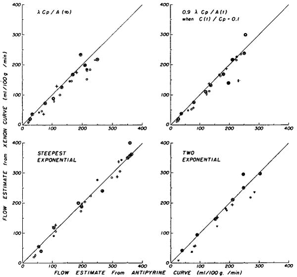
Flow calculated from exponential slope of portion of the curve centered at a time when C(t)/Cp = 0.3. (F = estimate flow and F_a = actual flow.) Data of each panel are summarized by regression equations given in Table 1. Each symbol refers to the same dog heart.

If monoexponential analysis were completely appropriate, all methods would yield similar results. All of these methods were applied by the digital computer using least-squares fitting of the exponential and therefore produced consistent results and eliminated personal bias (apart from the choice of the three methods). A comparison of the three methods is useful: the steepest slope gives the maximal overestimate; the slope at 0.3 Cp is more or less the standard method of applying monoexponential analysis; the slope at 70 seconds inevitably provides underestimates at high flow rates.

Two-Exponential Analysis

The recorded curves were fitted by the sum of the two exponentials by the equation:

$$\text{C}(\text{t})={\text{W}}_1{\text{f}}_1{\text{D}}_{1}exp(-{\text{f}}_1\text{t}/100{\lambda }_1)+{\text{W}}_2{\text{f}}_2{\text{D}}_{2}exp(-{\text{f}}_2\text{t}/100{\lambda }_2),$$ (2)

in which C(t) is count rate per minute, W₁ and W₂ are the relative weights of two types of homogeneous tissue, f₁ and f₂ are the flow rates (ml/100 g/min) through each of these two tissues, D₁ and D₂ are factors related to the dose of isotope injected and to the counting efficiency in each of the tissues (it is assumed that D₁ = D₂), t = time, and λ₁ and λ₂ (ml/g) are the tissue-blood partition coefficients for the two tissues or the volume of distribution of the isotope per gram of tissue. The assumptions involved in applying this formula will be discussed later. For this study, λ₁ = λ₂, with the same values as given above. From this formula the mean flow rate, F, is calculated by:

$$\text{F}={\text{W}}_1{\text{f}}_1+{\text{W}}_2{\text{f}}_2,$$ (3)

as Høedt-Rasmussen and associates (6) have done. The curve fitting was done by computer analysis using a variation of the semirandomized search technique of Hazelrig and associates (7), in which both exponentials are found simultaneously, rather than a peel-off technique, and using a weighting of 1 divided by the count rate at each point for the least-squares minimization, so that all data points have the same weight of influence on the curve fitting.

Analysis Using the Residue Function

The residue function, H*(t), the complement of the cumulative residue time distribution, H (t), has been described by Zierler (3) who called it l-H(t). It is the probability that the residence time exceeds t. When all of the isotopic indicator is within the organ at time zero, the curve recorded by an external counter is C(t) and

$$\text{H}\ast (\text{t})=\frac{\text{C}(\text{t})}{\text{C}(0)},$$

where C(0) is the count rate at time zero. H(t), the complement of H*(t), is the integral of the transport function, h(t), which is the probability density function of transit times through the organ.

Zierler's simple formula for calculating the organ flow is:

$$\text{F}=\frac{100\lambda \cdot \text{height}}{\text{area}}=\frac{100\lambda \text{C}(0)}{{\int }_0^{\infty }\text{C}(\text{t})\text{dt}}=\frac{100\lambda }{{\int }_0^{\infty }\text{H}\ast (\text{t})\text{dt}}.$$ (4)

The integral, ${\int }_0^{\infty }\text{H}\ast (\text{t})\text{dt}$, is the mean transit time. Because the long time required for complete washout of isotope makes it impractical to record the complete curve, several variations on the formula were tested. The most useful of these, given below by equation 7, is a variant of the intensity function which is used in chemical engineering to describe the probability of departure of indicator from systems such as chemical reactors (8).

Statistical Analysis

Linear regression equations for calculated flow rate, F, versus actual flow rate, F_a, were obtained for each isotope for each of the experimental situations described above for each heart. Multiple regression analyses were also performed to detect the influences of heart rate, perfusion pressure, drug infusion, heart weight, and actual flow rate on each of the methods of analysis of flow.

Results

One hundred and fifty-eight isotope disappearance curves were recorded from 13 dog hearts. Eight were isolated heart preparations, and five were perfused coronary preparations.

In Figures 2, 4, 7, 8, and 9 each symbol refers to the same dog heart. Except for Figures 8 and 9, all have the same abscissa in all four panels—the actual measured flow rate per 100 g of tissue, F_a. In Figures 2 and 7, the upper left panel represents 29 disappearance curves, the upper right panel 32, the lower left 40, and the lower right 57. In each, the upper right panel includes data acquired with the probe uncollimated and with it collimated to the apex.

Figure 4.

Mean flow from two-exponential analysis calculated by means of equations 2 and 3. Regression equations are given in Table 1.

Figure 7.

Flow rates estimated by height/area (H/A) method of equation 7 using T = time when C(T)/Cp = 0.1 (see Fig. 5, lower left). The consistent underestimation of flow indicates that λ should be larger than 0.7. Regression equations are given in Table 1, symbols in Figure 1.

Figure 8.

Comparison of flows estimated in the isolated heart preparation from antipyrine and xenon curves by four methods (see Table 2). The circled symbols indicate estimates from curves obtained by collimation on the apex. Each xenon curve was recorded 3 to 8 minutes after the antipyrine curve with which it was paired, at constant perfusion rate. Regression equations (Table 3) are given for F_Xe, the flows estimated from xenon curves, versus F_Ap, the flows estimated from antipyrine curves.

Figure 9.

Flows estimated from curves recorded from the whole heart plotted against those from the apical curves, by the method of equation 7 (as in Figure 7, using T at C(T)/Cp = 0.1).

Multiple regression analysis revealed no influences of drug infusion or blood pressure on estimations of coronary blood flow. The clearance of xenon from the whole heart tended to be slightly more rapid at high heart rates than at low heart rates, but no such tendency was seen for antipyrine or for xenon clearance from the apex.

Monoexponential Analysis

Exponential Slope at 30% of Peak Count Rate

This method of calculation yielded approximately linear relationships for F versus F_a (Fig. 2). The regression equations and the average ratios of estimated to actual flow rates, $\overline{\text{F}/{\text{F}}_{\text{a}}}$, are given in Table 1. As is particularly evident in the lower left panel, the scatter around the regression line for any single dog was less than for the group as a whole. For example, in the lower left panel the standard deviations for the closed circles, open circles, and inverted triangles were 13.3, 7.8, and 15.5 ml/100 g/min, respectively, while the standard deviation for the whole group was 31.4.

Table 1. Regression Equations Relating Estimated Flow to Actual Flow, F = y₀ + bF_a.

Method	Indicator	Site	Figure no. and panel	Intercept (y0)	Slope (b)	SD*	r	$\overline{\text{F}/{\text{F}}_{\text{a}}}$	N
Slope at 0.3 Cp	Xe	Apex	2 (LU)	−22	1.14	25	0.97	1.00	29
	Xe	Whole	2 (LL)	−39	0.99	31	0.93	0.76	40
	Ap	Apex and whole	2 (RU)	−25	1.06	27	0.96	0.91	32
	Xe	Coron.	2 (RL)	16.4	0.80	22	0.95	0.90	57
Steepest exponential slope	Xe	Apex		2.8	1.21	21	0.98	1.23	29
	Xe	Whole		−11	1.06	39	0.91	1.00	40
	Ap	Apex and whole		−5	1.19	22	0.98	1.16	32
	Xe	Coron.		28	0.84	19	0.96	1.00	57
Two-exponential equation	Xe	Apex	4 (LU)	−7	1.0	16	0.98	0.95	27
	Xe	Whole	4 (LL)	−19	0.77	2.3	0.94	0.64	37
	Ap	Apex and whole	4 (RU)	−6	0.94	23	0.96	0.91	25
	Xe	Coron.	4 (RL)	21	0.64	23	0.96	0.77	56
H/A (equation 7)	Xe	Apex	7 (LU)	−10	0.89	16	0.98	0.82	29
	Xe	Whole	7 (LL)	−25	0.80	24	0.94	0.66	40
	Ap	Apex and whole	7 (RU)	−9	0.83	18	0.97	0.78	32
	Xe	Coron.	7 (RL)	18	0.68	14	0.97	0.78	57

^*SD = standard deviation from regression; r = correlation coefficient; N = number of observations. Coron. refers to estimates obtained in the perfused coronary artery preparation, CP is the peak count rate, and H/A is height/area analysis. Xe = xenon; Ap = antipyrine. Panels referred to are LU, left upper; LL, left lower; RU, right upper; RL, right lower.

In the perfused coronary preparation only (not in the isolated heart), all methods of analysis resulted in an estimated best straight line with a positive ordinate intercept (for example, Fig. 2, lower right panel).

Steepest Exponential Slope

The estimated flow rate, F, was approximately linearly related to the actual flow rate, F_a. As above, better linear relationships are obtained for individual dogs than for the whole group. The results obtained by this method on the isolated heart preparation provided estimates averaging about 20% higher than from the slope at 0.3 Cp. The regression equations are given in Table 1 for comparison with those of the previous method.

Exponential Slope at 70 Seconds after Injection

Because all of these disappearance curves (Fig. 1) have gradually decreasing semilogarithmic slopes and because the washout is fastest for the highest flow rates, it might be expected that the estimates made at any specific time after injection would be relatively less for the higher flow rates. At high flow rates, the count rates at 70 seconds after injection were less than 10% of peak count rates. By this method one can obtain estimated flow rates which are virtually independent of the actual flow rates. For xenon washout from the whole isolated heart and from the perfused coronary, no estimate of F greater than 120 ml/100 g/min was obtained, even with F_a = 360 ml/100 g/min. The deviation from a single exponential washout was considerable even at flow rates as low as 150 ml/100 g/min.

Although this last test illustrates that monoexponential analysis is invalid in theory and that it should be applied with some caution to the heart, it is also apparent that the maximal overestimates (steepest-slope method) were not much greater than those of the most commonly accepted method (slope at 0.3 C_p) and both methods gave values of flow near the actual value. Moreover, it will be shown in the discussion that the major portion of the deviation from the line of identity in Figure 2 can be corrected by the use of the correct partition coefficient.

Two-Exponential Analysis

Figure 3 shows washout curves (continuous lines), for antipyrine and xenon from the whole isolated heart, fitted with equation 2 (the squares, plotted at intervals three times the length of the experimental intervals). The xenon and antipyrine curves have different shapes although all four sets of curves were from the same heart and the experiments were paired at constant flow, the antipyrine injection preceding the xenon injection by 3 to 8 minutes. The antipyrine curves were consistently straighter on semilogarithmic plots than were the xenon curves. For these curves the same partition coefficients (0.7 for xenon and 1.0 for antipyrine) were used for both compartments. This is reasonable for antipyrine because the partition coefficients for muscle and for fat do not differ. The more marked levelling off of the disappearance curve for xenon after the first minutes might be expected because of its higher partition coefficient for fat and the relatively lower blood flow rate in adipose tissue. For xenon, the partition coefficient for fat may be as high as 8.0 (9), but when such a value was used for λ₂, flow estimates for this compartment, f₂, were 100 to 500 ml/100 g/min, which are obviously ridiculously high. Thus, although fat may contribute to the prolongation of the disappearance slope, it cannot be considered as a second compartment with flow-limited exchange. The evidence provided by Tønnesen and Sejrsen (10) on clearance curves in the gastrocnemius before and after excision of visible fat would support this view. A few curves (13 of the 158) could not be closely fitted with a two-exponential equation and were omitted from the analysis.

Figure 3.

Two-exponential curves (equation 2) fitted to four pairs of isotope disappearance curves from one isolated heart experiment. The antipyrine-¹²⁵I was injected intra-arterially 3 to 8 minutes before the ¹³³Xe injection; flow rate and perfusion pressure were constant for each pair of curves. Equation 3 has been fitted to the xenon count rates, C_Xe, and to the antipyrine count rates, C_Ap, and plotted at every third point. For an example, the equations for the curves of the left upper panel are: C_Ap(t) = 1,160[0.32(47)exp(−.47t/λ) + 0.68(17) exp(−.17t/λ)]; C_Xe(t) = 1,200[0.43(18.3)exp(−.18/λ) + 0.57(2)exp(−.02t/λ)]. F̄_X and F̄_A are flows calculated by equation 3 for xenon and antipyrine curves, respectively.

Figure 4 shows the mean flow rate calculated by equation 2 plotted against the actual flow rate in the same four situations as shown in Figure 2. Disappointingly, the results are no less scattered than those obtained by single exponential analysis using either the steepest slope or the slope at 30% of peak (correlation coefficients and standard deviations not significantly different). The slopes of the regression lines are less, because the tails of the curves influence the estimate of F. Use of a higher value for the partition coefficient, which will be argued in the discussion to be proper, brings the estimates close to the line of identity.

Height/Area Analysis (Residue Function)

In Figure 5, four variations on the theoretical approach are illustrated. The classical method as described by Zierler (3) (equation 4) is modified in the left upper panel in recognition of the fact that the area integration must end at a finite time, T:

Figure 5.

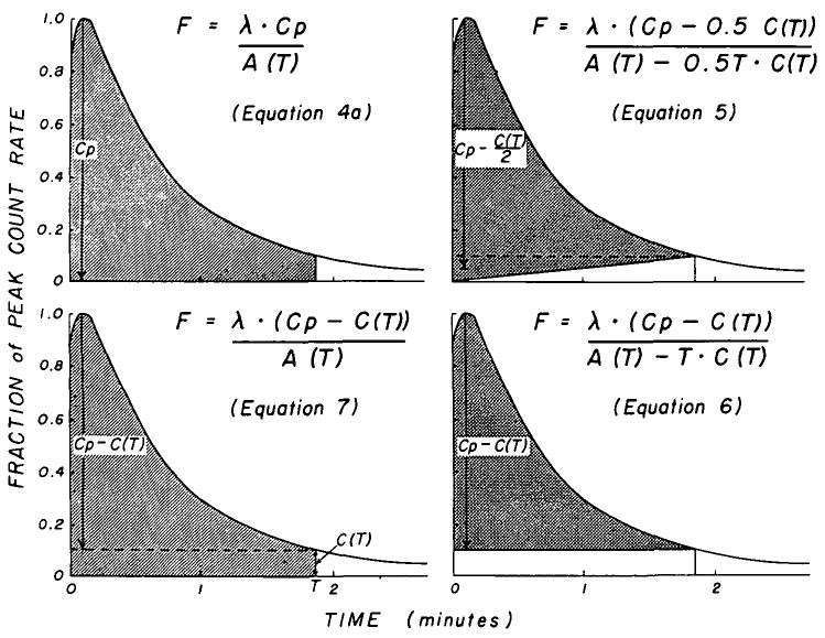
Geometric representation of four variations of the height/area (H/A) formula. The shaded portion represents the area in the denominator of each equation; the vertical arrow represents the height, H. In each, the area increases as the integration period lengthens and in all but the original method (upper left) the height used in the calculation also increases. F is in ml/g/min.

$$\text{F}=100\lambda \text{Cp}/\text{A}(\text{T})$$ (4a)

in which the area $\text{A}(\text{T})={\int }_0^{\text{T}}\text{C}(\text{t})\text{dt}$ and Cp = peak count rate. In the upper right and lower right panels, respectively, are illustrated equations 5 and 6:

$$\text{F}=\frac{100\lambda \left[\text{Cp}-0.5\text{C}(\text{T})\right]}{\text{A}(\text{T})-0.5\text{T}\cdot \text{C}(\text{T})}$$ (5)

$$\text{F}=\frac{100\lambda \left[\text{Cp}-\text{C}(\text{T})\right]}{\text{A}(\text{T})-\text{T}\cdot \text{C}(\text{T})}$$ (6)

The method which we think may be the most useful is given by equation 7 (6) and illustrated in the lower left panel:

$$\text{F}=100\lambda \left[\text{Cp}-\text{C}(\text{T})\right]/\text{A}(\text{T}).$$ (7)

Sensitivity of Height/Area Methods to Length of Observation Period

In Figure 6 are shown the flow rates calculated by these four formulas (equations 4a, 5, 6, and 7) for one isolated heart preparation using xenon injections at a wide variety of actual flow rates. The use of the fractional height, C(T)/Cp, as abscissa compresses the very long, drawn-out tails of the concentration-time curves. In all four formulas the denominator increases with increasing total integration time, most rapidly in equations 5 and 6. The numerator of equation 4a is independent of time, but in equations 5, 6, and 7 it increases. The magnitude of the downward slopes of the lines in Figure 6 indicates the sensitivity of each method to the time or level of C(T)/Cp.

Figure 6.

Dependency of flow estimation by height/area (H/A) on relative count rate at time, T, during tail of curve, for the four variations of the H/A method shown in Figure 5. Each line represents the late portion of one xenon washout curve and all are from the same isolated heart. The numerals on each line represent the actual flow rate, F_a, and the ordinate is the ratio of estimated to actual flow, F/F_a. C(T)/Cp is zero when the isotope washout curve has returned to the base line, and a close approximation to the F/F_a that would be obtained is given by extrapolating each line to C(T)/Cp = 0, for example, at the point F₀ (upper left). Only one method (lower left) is insensitive to the level of C(T)/Cp at which the formula is applied.

The data of the upper left panel show that for this isolated heart experiment equation 4a provides a correct estimate of flow (100% of the measured flow) when the height of the curve at the end of the integrating period is still between 25 and 15% of the peak height, so that ordinarily one will obtain significant underestimations (10 to 30%) if one extends the time for observations and integration until the tail is only 5% of the peak height. With C(T)/Cp = 0.1, the flow estimates are those at the intersections (for example, F₁₀) of the estimates with the vertical line at C(T)/Cp = 0.1. Even at this level, F/F_a averaged 0.91 for xenon at the apex and for antipyrine, 0.72 for xenon from the whole heart, and 0.87 for xenon from the perfused coronary. Equations 5 and 6 (Fig. 6 right-hand panels) show even steeper slopes and greater sensitivity to the point of termination of the integration.

Equation 7 (Fig. 6 lower left panel) produces lines that are flat on this plot and therefore provides estimates of flow rate that are virtually independent of C(T)/Cp. The horizontal nature of the relationship indicates that the washout curves are fairly close to monoexponential over this limited segment of the tail. Flow values obtained when C (T)/Cp = 0.1 were about 20% less than F_a, as shown in Figure 7. While the standard deviations are little better than for the above two methods, the method has the great advantage that the estimates were within 5% of the same value whether C(T)/Cp = 0.1 or 0.25. Therefore, equation 7 offers the great convenience of providing estimates of flow rate from data acquired over relatively short periods, without any apparent loss of accuracy. Similar conclusions may be drawn from the data acquired from all the experiments.

Extrapolation to Complete Washout

Straight lines were fitted by the method of least squares to the line relating flow rate, F, estimated by equation 4a, to C(T)/Cp for each washout curve, as illustrated for the uppermost line of the upper left panel of Figure 6. Linear extrapolation to C(T)/Cp = 0 provides an estimate of flow rate (for example, F₀) which is close to the values which would be obtained by recording for a very long time, as Zierler's theory requires. Consistent underestimations were obtained, F/F_a averaging 0.75 for xenon at the apex and for antipyrine, 0.55 for xenon from the whole heart, and 0.69 for xenon from the perfused coronary. These ratios would be much improved if a λ of 0.9 were used.

Antipyrine Versus Xenon Clearances

Although some actual differences in the shapes of the disappearance curves of xenon and antipyrine were seen (Fig. 3), these two isotopes did not generally provide very different estimates of flow (Fig. 8, and Tables 2 and 3). For curves recorded over the apex of the isolated heart preparation there was no difference between the unpaired means of the ratios $(\overline{\text{F}/{\text{F}}_{\text{a}}})$ for xenon and antipyrine (last two columns of Table 2), but for curves recorded from the whole isolated heart the means of the ratios for xenon were lower (P < 0.01) than those for antipyrine (Table 2).

Table 2. Mean Ratios (± sd) of Calculated to Actual Flow $\overline{(F/F_a)}$ Rates by Four Methods^*.

Method	Open-chest coronary perfusion (xenon) (N = 57	Isolated heart
		Whole		Apex
		Xenon (N = 40)	Antipyrine (N = 19)	Xenon (N = 29)	Antipyrine (N = 12)
Exp. slope at 0.3 Cp (Fig. 2)	0.94† ±.17	0.70†‡ ±.22	0.82† ±.17	0.96‡ ±.18	0.93 ±.15
Two-exp. (Fig. 4)	0.81† ±.15	0.61‡§ ±.17	0.84†§ ±.16	0.94†‡ ±.10	0.94 ±.11
H/A, eq. 4a	0.73† ±.13	0.52†‡§ ±.12	0.69†§ ±.13	0.75†‡ ±.12	0.77† ±.10
H/A, eq. 7 (Fig. 7)	0.82† ±.14	0.62†‡§ ±.16	0.73†§ ±.14	0.80†‡ ±.13	0.80† ±.10
Mean of four methods	0.82	0.61	0.77	0.86	0.87

^*Because, in general, the ratio F/F_a was lower at low perfusion rates, the mean ratios $\overline{\text{F}}/\overline{{\text{F}}_{\text{a}}}$ are lower than the ratios of the means $\overline{\text{F}}/\overline{{\text{F}}_{\text{a}}}$.

^†Ratio is different from 1.0 (P < 0.01).

^‡Ratio from apical curves differs from whole heart ratio for same indicator (P < 0.01).

^§Ratio for xenon data differs from antipyrine ratio from same location (P < 0.01). Abbreviations and symbols as in Table 1.

Table 3. Regression Equations Relating Xenon to Antipyrine Flow Estimates: F_Xe = y₀ + bF_Ap.

Fig. 8; panel	Equation	Whole heart (N = 15)				Apex (N = 10)
		yo	b	sd	r	yo	b	sd	r
LU	4a	−9.1	0.90	14.1	0.98	−4.1	1.02	20	0.98
RU	7	−18	1.08	9.1	0.99	−12	1.11	21	0.97
LL	1	−13	1.04	17	0.99	−9	1.04	19	0.99
RL	2	−16	0.93	14	0.98	−5	1.05	20	0.98

^*See Figure 8; panels and other abbreviations as in Table 1.

The average ratio of F_Xe/F_Ap from whole heart curves was less for those methods which utilize the tails of the recorded curves (Fig. 8: equation 4a, upper left panel; equation 2, lower right panel) than for the method which used only the initial portion of the downslope (Fig. 8: equation 1, lower left panel). Since equation 1 provides a maximal estimate which is necessarily an overestimate of the flow, it is apparent that the λ of 0.7 for xenon is erroneously low for observations made from the whole heart (see Discussion). No differences were observed for the apex ( $\overline{{\text{F}}_{\text{Xe}}/{\text{F}}_{\text{Ap}}}=0.98$, 1.0, 1.0, and 1.02 for equations 4a, 7, 1, and 2, respectively).

A paired comparison of clearances estimated by applying equation 7 to the curves obtained simultaneously from the apex and whole heart via two detectors is given in Figure 9. The average ratio of flow estimates from whole heart curves to those from apex curves is 0.81 ± 0.12 for xenon and 0.91 ± 0.11 for antipyrine. The regression equations are statistically different for the two indicators. These data and the unpaired comparison of the upper left and lower left panels of Figures 2, 4, and 7 suggest that the fatty tissue, in which xenon is highly soluble and which is mainly around the base of the heart and the large coronary vessels, is the main source of the difference between disappearance curves for antipyrine and xenon, and that the partition coefficient used is inappropriately low for the basal region of the heart. These suggestions are compatible with the conclusion, derived from the two-compartmental analysis, that fat alone does not form the second “uniformly mixed compartment.” A relatively low flow through a region with a higher than average proportion of adipose tissue is sufficient to explain the differences between the antipyrine and xenon curves.

Table 2 summarizes the results on the estimates of flow provided by the four most important methods.

Discussion

The isolated heart preparation was chosen for these experiments because it provided a stable, working muscle with a relatively high ratio of blood flow rate to volume, which could be varied over a wide range. The high capillary density and the dearth of arteriovenous shunts make it unlikely that either slow diffusion or arteriovenous shunting would affect the myocardial clearance of such highly diffusible substances as xenon and antipyrine.

The deviation of the observed antipyrine and xenon curves from a single exponential is probably due primarily to the existence of inhomogeneity of regional perfusion such as was observed by Thompson and associates (11). Other factors also can play a role; when there is either limited permeability of the capillary wall or slow diffusion in the tissue, the effect on the shape of the curves is the same as perfusion inhomogeneity. A chemical combination of the indicator with a less diffusible substance in the tissue will have the same effect. All of these situations produce washout curves with exponential slopes which are steeper initially than later. All also vitiate the primary assumption of complete mixing within the organ.

Even when a monoexponential curve is obtained, its slope does not necessarily provide an estimate of flow. Perhaps the situation in which a monoexponential curve is the most likely is one in which the slope has no relation to flow at all. This occurs in organs where there is countercurrent exchange between inflowing and outflowing vessels (venoarterial shunting), which vitiates the fundamental assumption that the inflow concentration is zero. Here, the slope of the disappearance curve is a function of flow and of the efficiency of the countercurrent exchange, and the existence of a monoexponential curve does not imply that there is either uniform concentration throughout the organ or that flow can be estimated. Even if the tissue concentration were uniform, flow could be estimated from the slope only if the efficiency of the exchanger were zero; otherwise, as Aukland and Berliner (12) have pointed out, flow is underestimated. Although arteries and veins do lie in close proximity in the heart, the exchange between them must be negligible because use of the more readily diffusible indicator, xenon, results in less monoexponential curves and provides similar estimates of clearance.

It was originally intended that a comparison between intramuscular and intra-arterial introduction of the indicators might be made. In a series of ten preliminary experiments, using injections into the left ventricular muscle of the isolated perfused heart, 120 apparently reasonable curves were produced (Fig. 1, upper left), but the variation in the flow values estimated from these curves was so great that the intramuscular route was abandoned. While it might be argued that removal from an intramuscular depot is likely to be diffusion-limited, at least initially, it is perhaps more likely that perfusion inhomogeneity becomes more apparent when one makes observations from localized regions. A similar conclusion might be drawn from the results of Doutheil and Rohde (13), who found that after intra-arterial injection of ⁸⁵Kr the curves obtained by counting the beta radiation which came from only the outer 1 to 2 mm of myocardium were widely and randomly different from those simultaneously obtained by counting gamma emissions from krypton throughout the myocardial thickness.

Diffusion in the Myocardium

The three analytic approaches tested are all based on the assumption that flow is steady, which means that the flow through each capillary should be constant. Although flow through the perfusion pump varied less than 5% during each pump cycle, there is certainly much evidence to indicate that the capillary flow changes dramatically with each cardiac contraction (14). One might argue that the time required for reduction of the count rate to 5% of peak count rate included at least 100 beats when the flow rate was highest and up to 1,000 beats at low flow rates and, therefore, that the information content of washout curves at cardiac frequencies is negligible. But less material will be removed when capillary flow is variable than when it is steady at the same mean flow rate, unless there is diffusion equilibrium across the capillary membrane at the venous end of the capillary and throughout the tissue at even the highest flow rates. This systematic deviation from the mean would be most exaggerated if the compression of the contracting muscle had stopped the capillary flow and emptied the capillaries at the beginning of systole, as suggested by the flowmeter curves of Sabiston and Gregg (14), so that all the capillary flow occurred at doubly high rates during diastole only, a situation that could occur normally and is likely to occur with increased systemic pressures. It is therefore possible that, even when mean coronary flow is constant from beat to beat, a limitation in removal rate of a moderately diffusible substance might be manifested merely by an increase in aortic resistance or heart rate, which shortens diastole more than systole. However, no evidence for such a limitation was obtained by the methods used in this study.

The analytic methods are more seriously invalidated if there is continuous redistribution of flow by opening and closing of individual capillaries or arterioles, unless instantaneous diffusion equilibrium occurs despite sudden large changes in diffusion distances. Some idea of the time for near equilibrium to occur may be obtained by determining the time required, after induction of a sudden change of concentration within the capillary, for the concentration in the region supplied by the capillary to come within 1% of the concentration in the capillary. On the basis of Krogh's data (15) for capillary radius (4 × 10⁻⁴ cm) and for capillary density (16) (2,500/mm² of cardiac tissue), a diffusion coefficient (15) in tissue of 6 × 10⁻⁶ (which is near that for antipyrine), and Roughton's (17) equations 3-10 and 3-11 and Figure 1 for a cylindrical capillary in the axis of a cylinder of tissue 12μ in radius, the half-time for diffusion exchange would be about 0.04 second and the time required for the concentration in tissue at the outer edge of the cylinder to differ by less than 1% from the concentration in the capillary would be about 0.16 second. This is a significant fraction of the plasma transport time from the arterial to the venous end of the capillary and, while it was expected that there might be some evidence for a diffusion limitation at the highest flows (350 ml/100 g/min) and heart rates (200/min), there was no significant influence of heart rate and no diminution of clearance at high flows.

Nevertheless, a very small intratissue gradient must remain. If a capillary closes, the diffusion distance for the region it supplies approximately doubles, and the time calculated for equilibrium in this specific region increases to about 2.0 seconds, which is now very significant relative to capillary transit time even though small compared to washout time. While the closure of even 20 or 30% of capillaries would be undetectable at low flow rates, at which the removal rate is limited by flow, the effect might be expected to show up at high flow rates. The linear relationships between estimated and actual flow rates in Figures 2, 4, and 7 are therefore evidence that at high flow rates there is no closure of a significant fraction of capillaries, periodically or ergodically, unless the duration of such closure is somewhat less than transcapillary transit times which could be as small as 0.3 second in these circumstances.

All these graphs and all these methods of analysis showed no definite indication of a diffusion limitation to the removal rate of these two diffusible indicators at the highest flow rates obtained in these experiments. The differences in the shapes of disappearance curves of antipyrine and xenon and of the ratios of F/F_a are probably explicable in terms of differences in distribution to fatty tissues and will be discussed below.

At high flows, the estimates of flow from curves from the cardiac apex in the isolated heart preparation (upper left panels of Figures 2, 4, and 7) were closer to the line of identity than those from the perfused coronary artery preparation (lower right panels of the same figures) but the mean values of F/F_a were not significantly different (Table 2). The difference is also seen as a difference between the slopes of the regression lines. One explanation may be based on the expectation of constancy of pulmonary washout of xenon from the perfused coronary preparation. At high coronary flow rates, the xenon in the lung within the field of the detector would result in a relative prolongation of the downslope. Another likely possibility is that the region perfused by the anterior descending coronary artery is dependent on the perfusion pressure, because, at high pressures, blood from this artery passes through collaterals supplying the adjacent region of the myocardium and reduces the ratio of perfused artery flow to mass of myocardium weighed at the end of the experiment. Contrarily, when the perfusion pressure is low, collaterals in contiguous regions being supplied at higher pressure from the dog's aorta will deliver blood to regions normally supplied by the anterior descending coronary artery. Such phenomena would readily explain not only the slope of F versus F_a in the lower right panels of Figures 2, 4, and 7, but also the positive ordinate intercepts on the regression lines. In none of the experiments and with none of the methods of analysis were the flow estimates with low F_a as small with the perfused artery as with the isolated heart preparation, strongly suggesting that collateral flow contributed significantly. Although this contribution could be estimated by taking into account the slopes of the regression lines, the intercepts, and the relative perfusion pressures, it was thought that the influence of too many other variables would make such computations meaningless.

Another possibility that applies most particularly to a comparison of clearances from the apex versus the whole heart is simply that the abscissa of the upper left panels is not quite appropriate: F_a, the actual flow rate, represents the mean flow rate for the whole isolated heart including the basal skeleton, a small rim of aorta and pulmonary artery, the valves, and the basal fat. No parts of these structures, which have low blood flow requirements, are included in the collimated apical field, and the flow rate in this muscle might easily be 20% greater than the mean rate for all tissues of the heart. This possibility, combined with a higher mean partition coefficient for xenon at the base of the heart (due to its higher fat content), may contribute to the difference between the flow rates estimated from the apex and from the whole heart.

The Partition Coefficient

The methods for calculation of flow are dependent on the use of the appropriate partition coefficient. In this study λ is considered to be the ratio of solubility in tissue to that in blood. Traditionally, values for λ obtained under static equilibrium conditions are equal to the partition coefficient. But it will be seen that when the situation is dynamic, λ may be dependent in a complex fashion on the relative amounts of different tissues in the organ, the time after injection, and the degree of achievement of equilibrium between blood and each type of tissue. Errors due to these three sources may either summate or offset one another. Each source will be considered in turn.

Consider the case in which there is instantaneous and continuous equilibrium between capillary blood and tissue. When an organ consists of two or more types of tissue the appropriate partition coefficient, λ_organ, is a weighted mean of the partition coefficients, λ_i, for the individual tissues. The weighting is the same whether the tissues are intimately mixed and supplied by the same capillary or are separated, are without interdiffusion, and are supplied by separate capillaries. The argument for separated tissues is as follows:

Let W_i = grams of tissue i per gram of organ, λ_i = its partition coefficient, f_i = its blood flow per gram of tissue i, and M = amount of injected indicator. From Zierler's formula,

$${\text{f}}_{\text{i}}={\lambda }_{\text{i}}{\text{H}}_{\text{i}}/{\text{A}}_{\text{i}}.$$ (8)

The height, H_i, contributed to the count rate measured by the external counting device with efficiency, E_i is

$${\text{H}}_{\text{i}}={\text{E}}_{\text{i}}{\text{Mw}}_{\text{i}}{\text{f}}_{\text{i}}/{\text{F}}_{\text{organ}}$$ (9)

where W_if_i/F_organ is the fraction of the dose delivered to tissue i and F_oragan is the organ blood flow per gram of organ. The curve area, from equation 8, is

$${\text{A}}_{\text{i}}=\frac{{\text{E}}_{\text{i}}{\text{Mw}}_{\text{i}}{\text{f}}_{\text{i}}{\lambda }_{\text{i}}}{{\text{f}}_{\text{i}}{\text{F}}_{\text{organ}}}={\text{E}}_{\text{i}}{\text{Mw}}_{\text{i}}{\lambda }_{\text{i}}/{\text{F}}_{\text{organ}}.$$ (10)

An external counter integrates or sums the counts from all the tissues so that H_organ = ΣE_iMw_if_i/F_organ and A_organ is the corresponding summation. Substituting into the equation for the whole organ gives:

$${\text{F}}_{\text{organ}}={\lambda }_{\text{organ}}\frac{{\text{H}}_{\text{organ}}}{{\text{A}}_{\text{organ}}}={\lambda }_{\text{organ}}\frac{\sum {\text{E}}_{\text{i}}{\text{Mw}}_{\text{i}}{\text{f}}_{\text{i}}}{\sum {\text{E}}_{\text{i}}{\text{Mw}}_{\text{i}}{\lambda }_{\text{i}}}$$ (11)

which is the equation that applies to the usual experimental situation. Since F_organ = Σf_iw_i, if equal efficiencies are assumed for all tissues, substitution in equation 11 and cancelling provide the solution,

$${\lambda }_{\text{organ}}=\sum {\text{w}}_{\text{i}}{\lambda }_{\text{i}},$$ (12)

which is the correctly weighted partition coefficient.

This equation holds only under conditions of equilibrium—that is, no net flux between blood and tissue—which, for a slug injection, occurs only when the experimental curve has been recorded until all of the isotope has been washed out. Under most circumstances this is impractical, and therefore the use of λ_organ (equation 12) will result in estimates of flow that are too high or too low depending on the relative washout rates of the constituent tissues. Let λ′_organ be considered as the functional value to be used, which is not necessarily the same as the ratio of solubilities or the ratio of concentrations at steady state, λ_organ. This question of the effective λ′_organ being a time-dependent value has been considered by H. K. Thompson (personal communication) who presented the following argument:

$$\lambda {\prime }_{\text{organ}}(\text{t})=\frac{{\text{C}}_{\text{organ}}(\text{t})}{{\text{C}}_{{\text{v}}_{\text{organ}}}(\text{t})}$$ (13)

by observation of the organ tissue concentration, C_organ, and the mixed venous outflow concentration, C_vorgan, at any time, t. That λ′_organ (t) is variable with time becomes more obvious when the tissue components are recognized. Substituting in equation 13,

$$\lambda {\prime }_{\text{organ}}(\text{t})=\frac{\sum {\text{w}}_{\text{i}}{\text{C}}_{\text{i}}(\text{t})}{\sum {\text{w}}_{\text{i}}{\text{f}}_{\text{i}}{\text{C}}_{{\text{v}}_{\text{i}}}(\text{t})}$$ (14)

$$=\frac{\sum {\text{w}}_{\text{i}}{\text{C}}_{\text{i}}(\text{t})}{\sum \left[{\text{w}}_{\text{i}}{\text{f}}_{\text{i}}{\text{C}}_{\text{i}}(\text{t})/{\lambda }_{\text{i}}\right]}.$$ (15)

Again, equation 15 only applies in the presence of a continuous tissue-blood equilibrium in each tissue and when diffusion from tissue to tissue is negligible.

This time-dependent λ′ (t) could be potentially useful when the recording of the curve cannot be continued to complete washout. What is needed is λ̄′(T), the average λ′ (t) throughout the curve from the beginning to the time, T, at which recording was stopped. This can be obtained by integration of Thompson's equation (equation 15):

$$\overline{\lambda }\prime (\text{T})=\frac{1}{\text{T}}{\int }_0^{\text{T}}\left(\frac{\sum \left[{\text{w}}_{\text{i}}{\text{C}}_{\text{i}}(\text{t})\right]}{\sum \left[{\text{w}}_{\text{i}}{\text{f}}_{\text{i}}{\text{C}}_{\text{i}}(\text{t})/{\lambda }_{\text{i}}\right]}\right)\text{dt}.$$ (16)

As T approaches infinity, λ̄′(T) approaches λ_organ as given by equation 12. When T is finite and there is some knowledge of the values of w_i, f_i, and λ_i, then at least directionally correct estimates of λ̄′(T) may be used instead of λ_organ in the various formulae.

It is clear the λ′_organ (t) obtained early in the disappearance curve will be weighted by those tissues into which the indicator has moved quickly, and λ′_organ (t) obtained late will be closer to the λ_i of the tissues cleared last, which will be those with the lowest ratios of flow to λ_i. This point is illustrated by data from four hearts stopped and quickly dissected soon after intra-arterial xenon injections. In one heart through which the flow was 223 ml/100 g/min, the flow was stopped abruptly 30 seconds after injection, at which time the count rate was 30% of the peak rate. The count rates per gram of adipose tissue at the base of the heart and around the large coronary arteries were 3.1 times those for various portions of ventricular muscle. In three other hearts the flow was stopped when the count rate was 3 to 10% of the peak rate, the flow rates being 210, 150, and 209 ml/100 g/min and the times of stoppage 100, 120, and 200 seconds after injection. In these, adipose tissue count rates averaged 9.5, 9.0, and 10.0 times those of muscle. Three conclusions may be drawn: (1) diffusion of xenon from muscle or blood-vessel wall to adipose tissue has occurred in the first 30 seconds because the ratio 3.1 is higher than the expected ratio (< 0.05) of amounts of indicator delivered by the blood to fat and muscle; (2) the xenon in muscle and that in adipose tissue are not equilibrated with each other in the early portion of the curve because the adipose-muscle ratio was only 3.1 at 30 seconds rather than near the ratio of solubilities (more than 10); and (3) the tails of the curves are more influenced by the amount of xenon in adipose tissue.

In addition to the lack of a muscle-fat equilibrium in the first seconds after injection, it is likely that the large intercapillary distances in adipose tissue result in a diffusion limitation. In dynamic experiments such as these, such a limitation results in a qualitatively predictable influence on the apparent λ′_organ (t). For any tissue i into which diffusion is slow, because of either large intercapillary distances or permeability barriers surrounding some regions, the ratio of tissue concentration to blood concentration, λ′_i (t), is less than the partition coefficient when the blood concentration is increasing soon after intra-arterial injection. After the time of the peak blood concentration resulting from a slug injection, λ′_i (t) will transiently be less than, then equal to, and then, for the remainder of the disappearance phase, greater than the partition coefficient. This phenomenon could contribute excessive area to the tail of the curve. A diffusion limitation in adipose tissue in these experiments should result in the ratio of concentrations of xenon or antipyrine in fat and in muscle being greater than λ_fat/λ_muscle in the late portions of the tail of the washout curve, a point on which we have no data.

A fourth possible influence on λ is the effect of plasma skimming and the differences in hematocrit value in different capillaries, because the partition coefficient for xenon is very dependent on hematocrit (10, 18).

It is therefore clear that fat around the major coronary branches and the base of the heart could and did contribute significantly to the tails of the curves. The possibility of some other causes was eliminated by simple experiments: (1) injection of xenon into the right ventricle showed it to be waslied out in a few seconds; (2) the total amount of xenon dissolved in the polyethylene tubing draining the left ventricle was inconsequential; and (3) the amount of xenon dissolved in the Silastic tubing attached to the cannulas to the aorta and pulmonary artery was small, was readily exchangeable, and was, in any case, shielded from the detecting crystal. The prolonged tails of the curves could also be a result of poor perfusion of some regions of the myocardium, but this is less likely in our nonworking preparation than in the working heart which Kirk and Honig (19) showed to have an increase in perfusion from subendocardial to subepicardial regions. By our crude method, in the nonworking, beating heart, portions of subendocardial muscle had xenon concentration levels no different from those of subepicardial muscle.

λ_organ for the heart

For indicators as highly diffusible as xenon it is not too unreasonable to make the approximation that λ_organ can be calculated by equation 12. (If this λ_organ is applied to analysis using the transport function, then, when the curve is not completed by washout to zero, there is the implicit assumption that there is a diffusion equilibrium during all phases of the curve.) With λ_fat = 8.0 and λ_muscle = 0.7, λ_organ is very dependent on the relative fractions of each tissue. Assuming that Conn's (9) value for λ of 0.72 was obtained on a heart with 1.5% fat, with 5% fat in muscle, λ_organ = 0.72 × (1 − 0.05 + 0.015) + 8.0 × (0.05 −0.015) = 0.98 and with 3% fat, λ_organ = 0.82. A value of 3% fat in the myocardium is too high for apical myocardium (20) but too low for basal regions which have variable large adipose deposits. It is therefore recommended that λ = 0.9 be used for the whole heart for application of these various formulae for calculating flow by clearance of xenon. This number cannot be ascertained with accuracy for any given heart and will be a gross underestimate in patients with large subepicardial and basal adipose tissue deposits or with fatty infiltration of the myocardium. For nonfatty hearts and at the apex in these dog hearts, Conn's value of 0.72 seems more appropriate.

When these values for λ are used, the values for F calculated for the whole heart come closer to F_a but still lie below the line of identity, as do those for antipyrine. This reduces the differences between F_Xe and F_Ap seen for the whole heart (uncircled symbols) in Figure 8. However, F still remains a little less than F_a whether xenon or antipyrine is used and with all methods of analysis (except the use of the steepest exponential slope, which should provide only overestimates). The explanations for this remaining error can only be guessed but include the problems of variable perfusion inhomogeneity and other types of unsteady state.

When using the transport function approach to the estimation of flow, the appropriate λ̄′_organ (T) is given by equation 16. For xenon in the heart, if muscle were cleared first and fat later and there were no diffusion between the two types of tissue, then λ′_organ (t) would be near 0.72 in the early part of the curve and near 8.0 in the final portions of the tail, while the time average, λ̄′_organ (T), would increase gradually toward λ_organ (given by equation 12) as T approaches the time of complete washout. When there is intertissue diffusion, even though it might not be sufficiently rapid to produce continuous equilibrium, at early times λ′_organ (t) is greater than 0.72 and at later times much less than λ_fat.

References

- 1.Herd JA, Hollenberg M, Thorburn GD, Kopald HH, Barger AC. Myocardial blood flow determined with krypton 85 in unanesthetized dogs. Am J Physiol. 1962;203:122. doi: 10.1152/ajplegacy.1962.203.1.122. [DOI] [PubMed] [Google Scholar]
- 2.Ross RS, Ueda K, Lichtlen PR, Rees JR. Measurement of myocardial blood flow in animals and man by selective injection of radioactive inert gas into the coronary arteries. Circulation Res. 1964;15:28. doi: 10.1161/01.res.15.1.28. [DOI] [PubMed] [Google Scholar]
- 3.Zierler KL. Equations for measuring blood flow by external monitoring of radioisotopes. Circulation Res. 1965;16:309. doi: 10.1161/01.res.16.4.309. [DOI] [PubMed] [Google Scholar]
- 4.Lassen NA, Klee A. Cerebral blood flow determined by saturation and desaturation with krypton85: An evaluation of the validity of the inert gas method of Kety and Schmidt. Circulation Res. 1965;16:26. doi: 10.1161/01.res.16.1.26. [DOI] [PubMed] [Google Scholar]
- 5.Kety SS. Measurement of regional circulation by the local clearance of radioactive sodium. Am Heart J. 1949;38:321. doi: 10.1016/0002-8703(49)90845-5. [DOI] [PubMed] [Google Scholar]
- 6.Høedt-Rasmussen K, Sveinsdottir Edda, Lassen NA. Regional cerebral blood flow in man determined by intra-arterial injection of radioactive inert gas. Circulation Res. 1966;18:237. doi: 10.1161/01.res.18.3.237. [DOI] [PubMed] [Google Scholar]
- 7.Hazelrig JB, Ackerman E, Rosevear JW. An iterative technique for conforming mathematical models to biomedical data. Proc 16th Ann Conf Eng Med Biol. 1963;5:8. [Google Scholar]
- 8.Naor P, Shinnar R. Representation and evaluation of residence time distributions. Ind Eng Chem Fundamentals. 1963;2:278. [Google Scholar]
- 9.Conn HL., Jr Equilibrium distribution of radioxenon in tissue: Xenon-hemoglobin association curve. J Appl Physiol. 1961;16:1065. doi: 10.1152/jappl.1961.16.6.1065. [DOI] [PubMed] [Google Scholar]
- 10.Tønnesen KH, Sejrsen P. Inert gas diffusion method for measurement of blood flow: Comparison of bolus injection to directly measured blood flow in the isolated gastrocnemius muscle. Circulation Res. 1967;20:552. doi: 10.1161/01.res.20.5.552. [DOI] [PubMed] [Google Scholar]
- 11.Thompson AM, Cavert HM, Lifson N, Evans RL. Regional tissue uptake of D2O in perfused organs: Rat liver, dog heart and gastrocnemius. Am J Physiol. 1959;197:897. doi: 10.1152/ajplegacy.1959.197.4.897. [DOI] [PubMed] [Google Scholar]
- 12.Aukland K, Berliner RW. Renal medullary countercurrent system studied with hydrogen gas. Circulation Res. 1964;15:430. doi: 10.1161/01.res.15.5.430. [DOI] [PubMed] [Google Scholar]
- 13.Doutheil U, Rohde R. Durchblutungs-bestimmung in oberflächlichen Myokardschichten und im gesamten Ventrikelmyokard mit Hilfe der Krypton-85-Auswaschtechnik. Arch Ges Physiol. 1966;290:258. [PubMed] [Google Scholar]
- 14.Sabiston DC, Jr, Gregg DE. Effect of cardiac contraction on coronary blood flow. Circulation. 1957;15:14. doi: 10.1161/01.cir.15.1.14. [DOI] [PubMed] [Google Scholar]
- 15.Kroch A. Rate of diffusion of gases through animal tissues, with some remarks on the coefficient of invasion. J Physiol (London) 1919;52:391. doi: 10.1113/jphysiol.1919.sp001838. [DOI] [PMC free article] [PubMed] [Google Scholar]
- 16.Krogh A. Anatomy and Physiology of Capillaries. 2. New Haven: Yale Univ. Press; 1929. p. 422. [Google Scholar]
- 17.Roughton FJW. Diffusion and chemical reaction velocity in cylindrical and spherical systems of physiological interest. Proc Roy Soc (London), Ser B. 1952;140:203. doi: 10.1098/rspb.1952.0059. [DOI] [PubMed] [Google Scholar]
- 18.Andersen AM, Ladefoced J. Relationship between hematocrit and solubility of 133Xe in blood. J Pharm Sci. 1965;54:1684. [Google Scholar]
- 19.Kirk ES, Honig CR. Nonuniform distribution of blood flow and gradients of oxygen tension within the heart. Am J Physiol. 1964;207:661. doi: 10.1152/ajplegacy.1964.207.3.661. [DOI] [PubMed] [Google Scholar]
- 20.Dible JH. Is fatty degeneration of the heart muscle a phanerosis? J Pathol Bacteriol. 1934;39:197. [Google Scholar]