Acceleration of Direct Reconstruction of Linear Parametric Images Using Nested Algorithms

Abstract

Parametric imaging using dynamic positron emission tomography (PET) provides important information for biological research and clinical diagnosis. Indirect and direct methods have been developed for reconstructing linear parametric images from dynamic PET data. Indirect methods are relatively simple and easy to implement because the image reconstruction and kinetic modeling are performed in two separate steps. Direct methods estimate parametric images directly from raw PET data and are statistically more efficient. However, the convergence rate of direct algorithms can be slow due to the coupling between the reconstruction and kinetic modeling. Here we present two fast gradient-type algorithms for direct reconstruction of linear parametric images. The new algorithms decouple the reconstruction and linear parametric modeling at each iteration by employing the principle of optimization transfer. Convergence speed is accelerated by running more sub-iterations of linear parametric estimation because the computation cost of the linear parametric modeling is much less than that of the image reconstruction. Computer simulation studies demonstrated that the new algorithms converge much faster than the traditional expectation maximization (EM) and the preconditioned conjugate gradient algorithms for dynamic PET.

1. Introduction

Conventional methods for generating parametric images in dynamic PET usually reconstruct a sequence of emission images from measured projection data first, and then fit the time activity curve (TAC) in each voxel to a linear or nonlinear kinetic model. To obtain an accurate estimate, the resolution and noise distribution of reconstructed emission images should be modeled in the kinetic modeling. However, exact modeling of noise distribution in emission images reconstructed by iterative methods is extremely difficult because the noise is space-variant and object-dependent. Often the space-varying noise variance and correlations between pixels are simply ignored in the kinetic modeling step, which leads to sub-optimal results. Direct reconstruction of parametric images from raw projection data solves this problem by combining kinetic modeling and emission image reconstruction into a single formula. It allows accurate modeling of noise statistics in data and hence is statistically more efficient [1–3].

Both linear and nonlinear temporal representations have been adopted in modeling TAC for parametric image reconstruction [4]. Here we focus on linear models. Compared with nonlinear models [2, 5–8], linear models, such as B-spline [9–12], spectral bases [13–16] and the Patlak model [3, 17], have a concave log-likelihood function, which can guarantee global convergence for maximum likelihood algorithms. For the Patlak model and the spectral analysis model, the model parameters (or combined) have physiological meanings related to the underlying biochemical process.

Researchers have extended gradient-based algorithms that were developed for static PET image reconstruction, such as EM (expectation maximization) and PCG (preconditioned conjugate gradient), to solve the optimization problems of linear parametric image reconstruction [3, 14, 17]. However, it has been found that the coupling between the emission image reconstruction and the temporal model can greatly affect the convergence rate of these algorithms, especially when the temporal basis functions are highly correlated, such as those used in the Patlak model and spectral analysis [18].

This paper presents two fast direct reconstruction algorithms to address this problem. In each iteration, the new algorithms decouple the linear kinetic modeling from the emission image reconstruction using the optimization transfer principle [23]. Once decoupled, the linear kinetic modeling can be run till convergence with little increase in the overall reconstruction time because the total computational cost is dominated by the forward and back projections in the image reconstruction step. The effectiveness of the new algorithms is demonstrated in the EM framework first and is extended to a conjugate gradient algorithm with line search to further improve the convergence rate. The resulting algorithms converge much faster than the traditional EM and PCG algorithms.

2. Reconstruction of Linear Parametric Images

Dynamic PET data are well modeled as a collection of independent Poisson random variables

$$y_{im}\sim \text{Poisson}\{{\overline{y}}_{im}\},i=1,\dots ,n_i;m=1,\dots ,n_m$$ (1)

with the expectation ȳ_im related to the unknown tracer distribution in time frame m, {x_jm}, through an affine transform

$${\overline{y}}_{im}=\sum _{j=1}^{n_j}{p}_{ij}{x}_{jm}+r_{im}$$ (2)

where p_ij, the (i, j)th element of the detection probability matrix P ∈ IR^n_i×n_j, is the probability of detecting an event from the jth pixel at the ith detector pair, and r_im accounts for the presence of scatters and randoms in the data. n_i, n_j, n_m are the numbers of detector pairs, image pixels, and time frames, respectively.

The time activity curve at each pixel can be modeled by linear or non-linear models. Here we focus on linear representations, i.e.,

$$x_{jm}=\sum _{k=1}^{n_k}{b}_{mk}{\theta }_{jk}$$ (3)

where b_mk is the (m, k)th element of a basis matrix B ∈ IR^n_m×n_k of which each column denotes a temporal basis function, and θ_jk is the coefficient (kinetic parameter) of the kth basis function at pixel j. n_k is the total number of basis functions. Then the expectation of the dynamic PET data is related to the kinetic parameters θ_jk through

$${\overline{y}}_{im}=\sum _{j=1}^{n_j}\sum _{k=1}^{n_k}{b}_{mk}{p}_{ij}{\theta }_{jk}+r_{im}$$ (4)

Let ȳ, y, r, x, and θ denote {ȳ_im}, {y_jm}, {r_im}, {x_jm}, and {θ_jk}, respectively, in the same fashion as ȳ = [ȳ₁₁, …, ȳ_ni1, ȳ₁₂, …, ȳ_ni2, …, ȳ_1nm, …, ȳ_ninm]^T. The expectation of dynamic PET data can be written in the following matrix-vector formula

$$\overline{\mathit{y}}=(\mathit{B}\otimes \mathit{P})\mathit{\theta }+\mathit{r}$$ (5)

where ⊗ denotes the Kronecker product.

Maximum likelihood (ML) estimate of the kinetic parameters can be found by

$$\widehat{\mathit{\theta }}=arg\underset{\mathit{\theta }}{max}\mathcal{L}(\mathit{y}\mid \mathit{\theta })$$ (6)

where ℒ(y|θ) is the Poisson log-likelihood function

$$\mathcal{L}(\mathit{y}\mid \mathit{\theta })=\sum _{m=1}^{n_m}\sum _{i=1}^{n_i}{y}_{im}log{\overline{y}}_{im}-{\overline{y}}_{im}$$ (7)

with a constant term omitted. To present the basic idea of the new algorithms, we consider here only the ML reconstruction, but the algorithms can be extended to maximum a posteriori (MAP) reconstruction.

3. The traditional EM and PCG Algorithms

3.1. The traditional EM algorithm

Since the dynamic data model in (5) is linear, the EM algorithm used in static PET can be directly applied to the reconstruction of linear parametric images by considering B ⊗ P as a single system matrix and inserting it into the EM algorithm [19], which results in the following update equation:

$${\widehat{\theta }}_{jk}^{n+1}=\frac{{\widehat{\theta }}_{jk}^n}{({\sum }_m{b}_{mk})({\sum }_i{p}_{ij})}\sum _i\sum _m{p}_{ij}{b}_{mk}\frac{y_{im}}{{\overline{y}}_{im}^n}$$ (8)

where the superscript n denotes the nth iteration and ${\overline{y}}_{im}^n$ is given in (5) with θ being θ̂ⁿ.

3.2. The traditional PCG algorithm

It is well known that the EM algorithm for static PET reconstruction belongs to scaled gradient ascent algorithms [20]. This is also true for the EM algorithm for dynamic image reconstruction shown in (8), which can be written as

$${\widehat{\theta }}_{jk}^{n+1}={\widehat{\theta }}_{jk}^n+q_{jk}^n\left[\sum _{i,m}{p}_{ij}{b}_{mk}\left(\frac{y_{im}}{{\overline{y}}_{im}^n}-1\right)\right]$$ (9)

where the term in the square brackets is the gradient of the log-likelihood function with respect to the kinetic parameters θ_jk and $q_{jk}^n$ is given by

$$q_{jk}^n=\frac{{\widehat{\theta }}_{jk}^n}{({\sum }_m{b}_{mk})({\sum }_i{p}_{ij})}.$$ (10)

An effective way to accelerate convergence of the EM algorithm is to use conjugate directions and line search, which results in the following preconditioned conjugate gradient (PCG) algorithm [21]:

• Step 1: Set the current update direction dⁿ to the EM direction ${\mathit{d}}_{\text{EM}}^n$,

  $${\mathit{d}}^n={\mathit{d}}_{\text{EM}}^n={\mathit{Q}}^n{\mathit{g}}^n$$ (11)

  where ${\mathit{g}}^n=\{g_{jk}^n\}$ denotes the gradient vector and ${\mathit{Q}}^n=\text{diag}\{q_{jk}^n\}$.

• Step 2: Construct the conjugate direction as

  $${\mathit{a}}^n={\mathit{d}}^n+{\gamma }^{n-1}{\mathit{a}}^{n-1}$$ (12)
  where a′ is initialized by a′ = d′. γⁿ⁻¹ can be calculated by a few choices [22]. Here we use the Polak-Ribiere form

  $${\gamma }^{n-1}=\frac{{({\mathit{g}}^n-{\mathit{g}}^{n-1})}^T{\mathit{d}}^n}{{({\mathit{g}}^{n-1})}^T{\mathit{d}}^{n-1}}.$$ (13)
• Step 3: The new estimate at iteration (n + 1) is calculated by

  $${\widehat{\mathit{\theta }}}^{n+1}={\widehat{\mathit{\theta }}}^n+{\alpha }^n{\mathit{a}}^n$$ (14)
  where αⁿ is determined by a line search

  $${\alpha }^n=arg\underset{\alpha }{max}\mathcal{L}(\mathit{y}\mid {\widehat{\mathit{\theta }}}^n+\alpha {\mathit{a}}^n).$$ (15)

A Newton-Raphson algorithm is used to find the optimum step size.

4. The Nested Algorithms

The traditional EM and PCG algorithms described in Section 3 can be slow in convergence for dynamic PET reconstruction, especially when the temporal basis functions are highly correlated [18]. To address this problem, we derive two nested algorithms in this section.

4.1. The nested EM algorithm

To derive the nested EM algorithm, we construct the following surrogate function (θ; θⁿ) for the log-likelihood function [1]

$${\mathcal{S}}_{\mathcal{L}}(\mathit{\theta };{\widehat{\mathit{\theta }}}^n)=\sum _j\left(\sum _i{p}_{ij}\right)\left(\sum _m{\widehat{x}}_{jm}^{n+1}log{x}_{jm}({\mathit{\theta }}_j)-x_{jm}({\mathit{\theta }}_j)\right)+\mathcal{L}(\mathit{y}\mid {\widehat{\mathit{\theta }}}^n)$$ (16)

where $x_{jm}({\mathit{\theta }}_j)={\sum }_{k=1}^{n_k}{b}_{mk}{\theta }_{jk}$ and ${\widehat{x}}_{jm}^{n+1}$ is defined as

$${\widehat{x}}_{jm}^{n+1}=\frac{x_{jm}({\widehat{\mathit{\theta }}}_j^n)}{{\sum }_i{p}_{ij}}\sum _i{p}_{ij}\frac{y_{im}}{{\overline{y}}_{im}^n}.$$ (17)

The above surrogate function (θ; θⁿ) minorizes the original log-likelihood function in (7) and satisfies

$$\mathcal{L}(\mathit{y}\mid \mathit{\theta })-\mathcal{L}(\mathit{y}\mid {\widehat{\mathit{\theta }}}^n)\ge {\mathcal{S}}_{\mathcal{L}}(\mathit{\theta };{\widehat{\mathit{\theta }}}^n)-{\mathcal{S}}_{\mathcal{L}}({\widehat{\mathit{\theta }}}^n;{\widehat{\mathit{\theta }}}^n).$$ (18)

The new kinetic parameter estimate at iteration (n + 1) can be obtained by maximizing (θ; θ̂ⁿ) with respect to θ. Since (θ; θ̂ⁿ) is separable in voxels, the maximization can be carried out voxel-by-voxel, i.e.,

$${\widehat{\mathit{\theta }}}_j^{n+1}=arg\underset{{\mathit{\theta }}_j}{max}\sum _m{\widehat{x}}_{jm}^{n+1}log{x}_{jm}({\mathit{\theta }}_j)-x_{jm}({\mathit{\theta }}_j)$$ (19)

which can be solved by the following EM-like update equation:

$${\widehat{\theta }}_{jk}^{n,l+1}=\frac{{\widehat{\theta }}_{jk}^{n,l}}{{\sum }_m{b}_{mk}}\sum _m{b}_{mk}\frac{{\widehat{x}}_{jm}^{n+1}}{x_{jm}({\widehat{\mathit{\theta }}}_j^{n,l})},l=1,\dots ,n_l$$ (20)

where l is the sub-iteration number and ${\widehat{\theta }}_{jk}^{n+1}\equiv {\widehat{\theta }}_{jk}^{n,n_l+1}$.

Since an EM-type iteration is nested in the M step, it is referred to as “nested EM” to distinguish it from the traditional EM described in Section 3. Each full iteration of the nested EM algorithm consists of one iteration of (17) and multiple iterations of (20). The first step (17) resembles an emission image reconstruction and the second step (20) is an update of the linear kinetic parameters based on the intermediate image { ${\widehat{x}}_{jm}^{n+1}$}.

It is interesting to note that the traditional EM algorithm in (8) can also be rewritten into the following two separate steps by using the intermediate image ${\widehat{x}}_{jm}^{n+1}$:

$${\widehat{x}}_{jm}^{n+1}=\frac{x_{jm}({\widehat{\mathit{\theta }}}_j^n)}{{\sum }_i{p}_{ij}}\sum _i{p}_{ij}\frac{y_{im}}{{\overline{y}}_{im}^n}$$ (21)

$${\widehat{\theta }}_{jk}^{n+1}=\frac{{\widehat{\theta }}_{jk}^n}{{\sum }_m{b}_{mk}}\sum _m{b}_{mk}\frac{{\widehat{x}}_{jm}^{n+1}}{x_{jm}({\widehat{\mathit{\theta }}}_j^n)}.$$ (22)

Therefore, the traditional EM algorithm in (8) is just a special case of the nested EM algorithm with n_l = 1.

Because the size of matrix B is much smaller than that of the system matrix P, the computational cost of (20) is much less than that of (17). Therefore, the nested EM algorithm can accelerate the convergence rate of the direct reconstruction by running multiple iterations of (20) without affecting the overall computational time. A similar concept to improve convergence speed was also used in the coordinate descent optimization for nonlinear kinetic models, where linear parameters were updated more often than nonlinear parameters [2].

4.2. The Nested Conjugate Gradient Algorithm

We extend the nested EM algorithm to a conjugate gradient algorithm described in Section 3.2. This is done by considering the nested EM algorithm as an implicit preconditioner and setting the direction vector dⁿ to the direction calculated by the nested EM, i.e.,

$${\mathit{d}}^n={\widehat{\mathit{\theta }}}_{\text{NestEM}}^{n+1}-{\widehat{\mathit{\theta }}}^n$$ (23)

where ${\widehat{\mathit{\theta }}}_{\text{NestEM}}^{n+1}$ is the new update of θ obtained by the nested EM algorithm using (20). Steps 2 and 3 of the PCG algorithm remain unchanged. The resulting algorithm is referred to as the nested CG algorithm to distinguish from the traditional PCG algorithm. Because of the incorporation of the nested EM direction, the nested CG algorithm is shown to converge much faster than the traditional PCG algorithm.

5. Simulation Results

To validate the proposed nested algorithms, we performed three different simulations: a two-pixel imaging problem, a Patlak parametric reconstruction, and a spectral image reconstruction.

5.1. Two-pixel dynamic imaging

We first illustrate the improvement of the proposed algorithms over the traditional algorithms using a toy example. We simulated a two-pixel dynamic imaging system. The system matrix and temporal basis functions are

$$\mathit{P}={\left[\begin{array}{ccc}0.5& 1& 0\\ 0.5& 0& 1\end{array}\right]}^T,\mathit{B}=\left[\begin{array}{cc}2& 1\\ 1& 2\end{array}\right].$$

The true kinetic parameters for the two pixels are

$${\mathit{\theta }}_1=\left[\begin{array}{c}0.5\\ 1\end{array}\right],{\mathit{\theta }}_2=\left[\begin{array}{c}0.7\\ 0.7\end{array}\right].$$

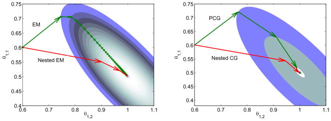
In the nested algorithms, 30 sub-iterations were used. Noise-free data were used in this example. Fig. 1 shows the isocontours of the likelihood function and the trajectories of the iterates for estimating θ₁ while keeping θ₂ fixed at its true values. The nested EM takes 6 iterations to converge to the true solution, while the traditional EM requires more than 60 iterations. For the conjugate gradient algorithms, the nested CG uses 3 iterations and the traditional PCG takes 9 iterations to converge. Since the PCG algorithm is usually much faster than the EM algorithm, we will only show comparisons between the PCG and the nested CG algorithms hereafter.

Figure 1.

Isocontours of the likelihood function of the toy problem and the trajectories of the iterates of the traditional EM and the nested EM (left), and the traditional PCG and the nested CG (right). The nested EM takes 6 iterations to converge to the final solution, while the traditional EM requires more than 60 iterations. For the conjugate gradient algorithms, the nested CG uses 3 iterations and the traditional PCG takes 9 iterations to converge.

5.2. Patlak image reconstruction

The Patlak graphical method is a linear technique which has been widely used in dynamic PET data analysis [24]. The slope of the Patlak plot is a very useful quantitative index for characterizing the kinetic properties of many PET tracers. It can be applied to blood flow data [25], FDG data [26], and has found applications in many disease studies [27, 28]. Under the Patlak plot model, the pixel-wise time acitivity curve c(t) can be described by

$$c(t)=K_i{\int }_0^t{C}_{\text{p}}(\tau )\text{d}\tau +b{C}_{\text{p}}(t),t>t^{\ast }$$ (24)

where C_p(t) is the blood input function, K_i is the Patlak slope, b is the intercept, and t^* is the time for the tracer to reach steady state. The two basis functions in the Patlak model are the blood input function C_p(t) and its integral. Both the PCG algorithm [3] and EM algorithm [17] have been developed for the Patlak parametric image reconstruction and have been shown to achieve better bias-variance trade-off compared with indirect methods, but suffer from slow convergence. Here we show that the nested algorithms can accelerate the convergence.

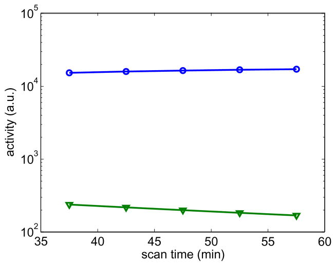
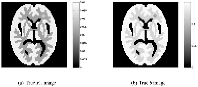
We simulated dynamic PET sinogram data using the same digital Hoffman brain phantom, kinetic parameters, scanning sequence, and blood input function as those used in our previous paper [3]. The corresponding Patlak basis functions B are shown in Fig. 2. Fig. 3 shows the true images of the Patlak slope K_i and the intercept b. A 25% spatially-uniform and temporally-varying background was added to the dynamic sinograms to simulate random and scattered events. Poisson noise was generated, which results in about 4 million events over a period of 25 minutes. We used the PCG and the nested CG algorithms to reconstruct the parametric images of the Patlak slope K_i and the intercept b from the noise-free and noisy sinogram data. The nested CG algorithm used 30 sub-iterations. In both reconstruction algorithms, the expectation of the background events is assumed known exactly and is modeled by the term r in equation (5). While in real situations, scattered and random events do not have a uniform spatial distribution, the correction scheme is the same once their expectations are properly estimated prior to reconstruction and we do not expect that the exact shape of the distribution would affect the relative performance between the two algorithms that are compared here.

Figure 2.

The basis functions used in the Patlak parametric image reconstruction.

Figure 3.

True parametric images of Patlak slope K_i (a) and the intercept b (b).

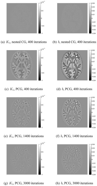
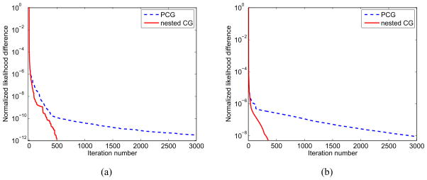
Fig. 4 shows the difference images between the true parametric images and the reconstructions of the noise-free data. When both algorithms were run for four hundred iterations, the nested CG results are much closer to the true images than those obtained by the traditional PCG algorithm. The large difference between the PCG reconstructions and the true images can be reduced by running the PCG algorithm for more iterations (e.g. 3000 iterations). This is also reflected by the plots of the normalized likelihood difference (NLD) as a function of iteration number n shown in fig. 5. The NLD is defined by

Figure 4.

Difference images of K_i and b reconstructed from noise-free sinograms using the PCG algorithm and the nested CG algorithm.

Figure 5.

Normalized likelihood difference of the Patlak parametric image reconstruction for the PCG and the nested CG algorithms: (a) noise-free data case; (b) noisy data case.

$$\mathit{NLD}(n)=\frac{\mathcal{L}(\widehat{\mathit{\theta }})-\mathcal{L}({\mathit{\theta }}^n)}{\mathcal{L}(\widehat{\mathit{\theta }})-\mathcal{L}({\mathit{\theta }}^0)},$$ (25)

where the reference likelihood ℒ(θ̂) is given by the likelihood of the PCG reconstruction with 5000 iterations. For the noise-free case, the PCG algorithm took 1400 iterations to reach a similar likelihood level as that achieved by the nested CG algorithm with 400 iterations. However, even with similar likelihood values, the images reconstructed by the two algorithm are still different as shown in fig. 4, because the two algorithms took different paths along the optimization process and the Patlak reconstruction problem is very ill-posed. For the noisy case, it took the PCG algorithm more than 3000 iterations to reach the likelihood level that is obtained by the nested CG algorithm with 300 iterations. Overall, the NLD plots show that the nested CG algorithm converges much faster than the traditional PCG algorithm for the Patlak image reconstruction.

5.3. Spectral image reconstruction

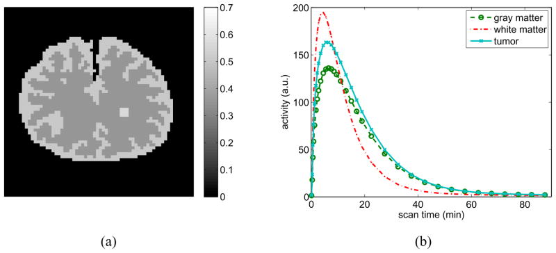
We also apply the nested CG algorithm to a spectral image reconstruction problem. A phantom shown in Fig. 6(a) was used to simulate a ¹¹C-labeled ligand-receptor binding kinetics in brain. The phantom consists of gray matter, white matter and a small tumor inside the white matter. The TACs of the gray matter and tumor region were generated using a two-tissue compartment model with an analytical blood input function [29]. The TAC of the white matter was generated using a one-tissue compartment model. The kinetic parameters used were K₁ = 0.06 min⁻¹, k₂ = 0.25 min⁻¹, k₃ = 0.11 min⁻¹, k₄ = 0.10 min⁻¹ for the gray matter region, K₁ = 0.11 min⁻¹, k₂ = 0.31 min⁻¹ for the white matter region, and K₁ = 0.08 min⁻¹, k₂ = 0.30 min⁻¹, k₃ = 0.11 min⁻¹, k₄ = 0.10 min⁻¹ for the tumor. The fractional volume f_v was set to zero for all regions. The dynamic PET data consists of 34 time frames over 90 minutes: 4×0.25 min, 4×0.5 min, 7×1 min, 5×2 mins and 14×5 mins. The regional TACs are shown in Fig. 6(b). These TACs were integrated for each frame and forward projected to generate dynamic sinograms. Random and scattered events were simulated by adding a 25% spatially-uniform and temporally-varying background to the sinograms. Poisson noise was then generated, which resulted in an expected total number of events over the 90 minutes equal to 50 million.

Figure 6.

The digital phantom (left) and regional time activity curves (right) used in the simulation for the spectral image reconstruction.

The spectral basis functions used in reconstruction are a set of exponential functions convoluted with the blood input function C_p(t),

$$b_k(t)={\phi }_{k}exp(-{\phi }_{k}t)\otimes C_{\text{p}}(t)$$ (26)

where φ_k denotes the rate constant of the kth spectrum. The advantage of using exponential bases is that they are consistent with compartmental models and the volume of distribution (VD) can be directly computed from the spectral coefficients by [30]

$$V_D=\sum _k{\theta }_k.$$ (27)

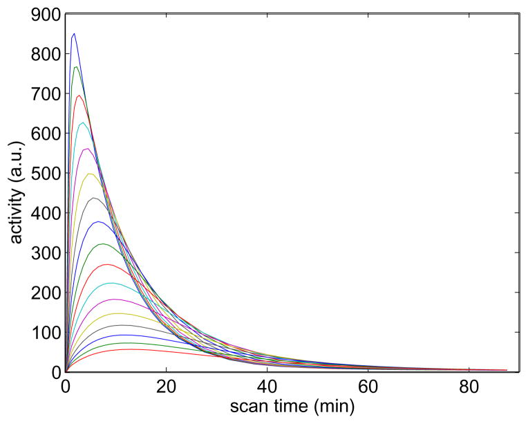
We used 50 spectral basis functions with rate constants log-uniformly distributed between 0.01 and 1.0. A representative subset of the basis functions are shown in figure 7. The data were reconstructed using both the PCG and nested CG algorithm. Fifteen sub-iterations were used in the nested CG algorithm.

Figure 7.

A representative subset of the basis functions used for the spectral image reconstruction.

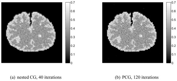
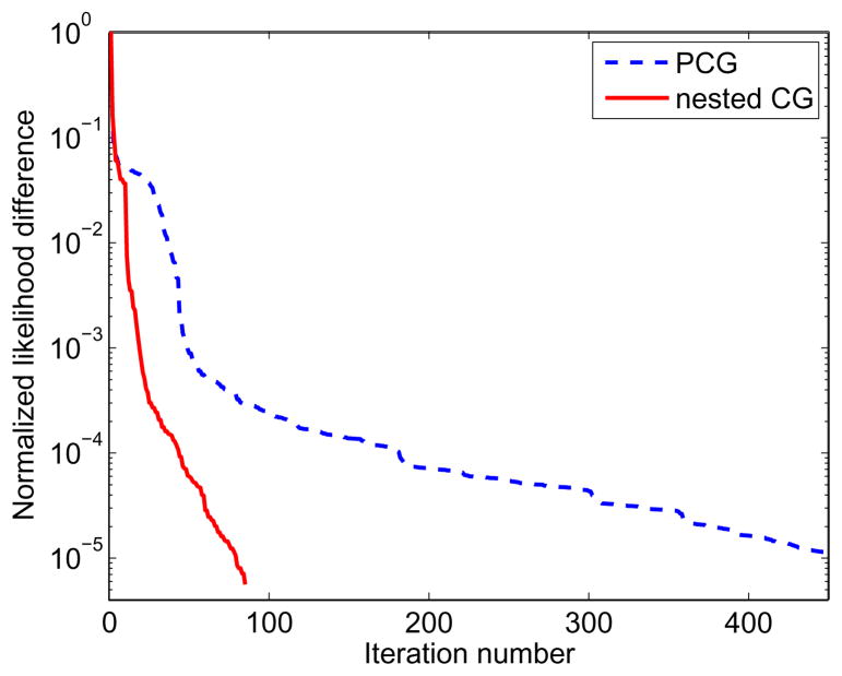
The parametric images of the volume of distribution reconstructed by the PCG and nested CG are shown in Fig. 8. To obtain these two images, the PCG reconstruction took 120 iterations, while the nested CG took 40 iterations. Fig. 9 compares the normalized likelihood difference (defined in equation (25)) of the traditional PCG algorithm and the nested CG algorithm for the spectral reconstruction. Here the reference likelihood in equation (25) was the likelihood achieved by the PCG reconstruction with 500 iterations. The plots clearly show that the nested CG algorithm achieves faster convergence rate than the traditional PCG algorithm.

Figure 8.

Reconstructions of the volume of distribution from a set of noisy sinogram data using the PCG and the nested CG algorithms.

Figure 9.

Normalized likelihood difference of the spectral parametric image reconstruction from a set of noisy data using the PCG and the nested CG algorithms.

6. Conclusion

We have developed a nested EM algorithm for direct reconstruction of linear parametric images from dynamic PET sinograms. The algorithm decouples the image reconstruction and kinetic modeling at each iteration and is faster than the conventional EM algorithm for reconstructing parametric images. We have further accelerated the nested EM algorithm using a conjugate gradient algorithm. Computer simulation studies have shown that the new algorithms converge much faster than the traditional EM and PCG algorithms for dynamic PET.

In this paper we have focused on maximum likelihood reconstruction. The algorithm can be extended to maximum a posteriori (MAP) reconstruction. Depending on whether the regularization is applied to the time activity curve or kinetic parameters, either equation (17) or (20) can be modified to accommodate the prior function.

References

- 1.Carson RE, Lange K. The EM parametric image reconstruction algorithm. Journal of America Statistics Association. 1985;80(389):20–22. [Google Scholar]
- 2.Kamasak ME, Bouman CA, Morris ED, Sauer K. Direct reconstruction of kinetic parameter images from dynamic PET data. IEEE Transactions on Medical Imaging. 2005;24(5):636–650. doi: 10.1109/TMI.2005.845317. [DOI] [PubMed] [Google Scholar]
- 3.Wang G, Fu L, Qi J. Maximum a posteriori reconstruction of the Patlak parametric image from sinograms in dynamic PET. Physics in Medicine and Biology. 2008;53(3):593–604. doi: 10.1088/0031-9155/53/3/006. [DOI] [PubMed] [Google Scholar]
- 4.Rahmim A, Cheng JC, Blinder S, Camborde ML, Sossi V. Statistical dynamic image reconstruction in state-of-the-art high-resolution PET. Physics in Medicine and Biology. 2005;50(20):4887–4912. doi: 10.1088/0031-9155/50/20/010. [DOI] [PubMed] [Google Scholar]
- 5.Reutter BW, Gullberg GT, Huesman RH. Kinetic parameter estimation from attenuated SPECT projection measurements. IEEE Transactions on Nuclear Science. 1998;45(6):3007–3013. [Google Scholar]
- 6.Vanzi E, Formiconi AR, Bindi D, Cava GL, Pupi A. Kinetic parameter estimation from renal measurements with a three-headed SPECT system: A simulation study. IEEE Transactions on Medical Imaging. 2004;23(3):363–373. doi: 10.1109/TMI.2004.824149. [DOI] [PubMed] [Google Scholar]
- 7.Reader AJ, Matthews JC, Sureau FC, et al. Iterative kinetic parameter estimation within fully 4D PET image reconstruction. 2006 IEEE Nucleal Science Symposium and Medical Imaging Conference; 2006. pp. 1752–1756. [Google Scholar]
- 8.Wang G, Qi J. Generalized algorithms for direct reconstruction of parametric images from dynamic PET data. IEEE Transactions on Medical Imaging. 2009;28(11):1717–1726. doi: 10.1109/TMI.2009.2021851. [DOI] [PMC free article] [PubMed] [Google Scholar]
- 9.Reutter BW, Gullberg GT, Huesman RH. Direct least-squares estimation of spatiotemporal distributions from dynamic SPECT projections using a spatial segmentation and temporal B-splines. IEEE Transactions on Medical Imaging. 2000;19(5):434–450. doi: 10.1109/42.870254. [DOI] [PubMed] [Google Scholar]
- 10.Reutter BW, Gullberg GT, Huesman RH. Effects of temporal modelling on the statistical uncertainty of spatiotemporal distributions estimated directly from dynamic SPECT projections. Physics in Medicine and Biology. 2002;47(15):2673–2683. doi: 10.1088/0031-9155/47/15/309. [DOI] [PubMed] [Google Scholar]
- 11.Nichols TE, Qi J, Asma E, Leahy RM. Spatiotemporal reconstruction of list-mode PET data. IEEE Transactions on Medical Imaging. 2002;21(4):396–404. doi: 10.1109/TMI.2002.1000263. [DOI] [PubMed] [Google Scholar]
- 12.Li QZ, Asma E, Ahn S, Leahy RM. A fast fully 4-D incremental gradient reconstruction algorithm for list mode PET data. IEEE Transactions on Medical Imaging. 2007;26(1):58–67. doi: 10.1109/TMI.2006.884208. [DOI] [PubMed] [Google Scholar]
- 13.Meikle SR, Matthews JC, Cunningham VJ, Bailey DL, Livieratos L, Jones T, Price P. Parametric image reconstruction using spectral analysis of PET projection data. Physics in Medicine and Biology. 1998;43(3):651–666. doi: 10.1088/0031-9155/43/3/016. [DOI] [PubMed] [Google Scholar]
- 14.Matthews J, Bailey D, Price P, Cunningham V. The direct calculation of parametric images from dynamic PET data using maximum-likelihood iterative reconstruction. Physics in Medicine and Biology. 1997;42(6):1155–1173. doi: 10.1088/0031-9155/42/6/012. [DOI] [PubMed] [Google Scholar]
- 15.Reader AJ, Sureau FC, Comtat C, Trebossen R, Buvat I. Joint estimation of dynamic PET images and temporal basis functions using fully 4D ML-EM. Physics in Medicine and Biology. 2006;51(21):5455–5474. doi: 10.1088/0031-9155/51/21/005. [DOI] [PubMed] [Google Scholar]
- 16.Reader AJ, Matthews JC, Sureau FC, Comtat C, Trebossen R, Buvat I. Fully 4D image reconstruction by estimation of an input function and spectral coefficients. 2006 IEEE Nucleal Science Symposium and Medical Imaging Conference; 2007. pp. 3260–3267. [Google Scholar]
- 17.Tsoumpas C, Turkheimer FE, Thielemans K. Study of direct and indirect parametric estimation methods of linear models in dynamic positron emission tomography. Medical Physics. 2008;35(4):1299–1309. doi: 10.1118/1.2885369. [DOI] [PubMed] [Google Scholar]
- 18.Tsoumpas C, Turkheimer F, Thielemans K. Convergence properties of algorithms for direct parametric estimation of linear models in dynamic PET. Nuclear Science Symposium Conference Record; 2007; 2007. pp. 3034–3037. [Google Scholar]
- 19.Shepp LA, Vardi Y. Maximum likelihood reconstruction for emission tomography. IEEE Transations on Medical Imaging. 1982 October;1(2):113–122. doi: 10.1109/TMI.1982.4307558. [DOI] [PubMed] [Google Scholar]
- 20.Kaufman L. Implementing and accelerating the EM algorithm for positron emission tomography. IEEE Transations on Medical Imaging. 1987 March;6(1):37–51. doi: 10.1109/TMI.1987.4307796. [DOI] [PubMed] [Google Scholar]
- 21.Mumcuoglu EU, Leahy R, Cherry SR, Zhou ZY. Fast gradient-based methods for Bayesian reconstruction of transmission and emission PET images. IEEE Transactions on Medical Imaging. 1994;13(4):687–701. doi: 10.1109/42.363099. [DOI] [PubMed] [Google Scholar]
- 22.Luenberger DG. Linear and Nonlinear Programming. 2. Addison-Wesley Publishing Company; 1984. [Google Scholar]
- 23.Lange K, Hunter DR, Yang I. Optimization transfer using surrogate objective functions. Journal of Computational and Graphical Statistics. 2000;9(1):1–20. [Google Scholar]
- 24.Patlak CS, Blasberg RG. Graphical evaluation of blood-to-brain transfer constants from multiple-time uptake data: Generalizations. Journal of Cerebral Blood Flow & Metabolism. 1985;5:584–590. doi: 10.1038/jcbfm.1985.87. [DOI] [PubMed] [Google Scholar]
- 25.Choi Y, Huang SC, Hawkins RA, Kuhle WG, Dahlbom M, Hoh CK, Czernin J, Phelps ME, Schelbert HR. A simplified method for quantification of myocardial blood-flow using Nitrogen-13-Ammonia and dynamic PET. Journal of Nuclear Medicine. 1993;34(3):488–497. [PubMed] [Google Scholar]
- 26.Choi Y, Hawkins RA, Huang SC, Gambhir SS, Brunken RC, Phelps ME, Schelbert HR. Parametric images of myocardial metabolic-rate of glucose generated from dynamic cardiac PET and 2-[F-18]Fluoro-2-Deoxy-D-Glucose studies. Journal of Nuclear Medicine. 1991;32(4):733–738. [PubMed] [Google Scholar]
- 27.Gill SS, Patel NK, Hotton GR, O’Sullivan K, McCarter R, Bunnage M, Brooks DJ, Svendsen CN, Heywood P. Direct brain infusion of glial cell line-derived neurotrophic factor in Parkinson disease. Nature Medicine. 2003;9(5):589–595. doi: 10.1038/nm850. [DOI] [PubMed] [Google Scholar]
- 28.Kordower JH, Emborg ME, Bloch J, Ma SY, Chu YP, Leventhal L, McBride J, Chen EY, Palfi S, Roitberg BZ, Brown WD, Holden JE, Pyzalski R, Taylor MD, Carvey P, Ling ZD, Trono D, Hantraye P, Deglon N, Aebischer P. Neurodegeneration prevented by lentiviral vector delivery of GDNF in primate models of Parkinson’s disease. Science. 2000;290(5492):767–773. doi: 10.1126/science.290.5492.767. [DOI] [PubMed] [Google Scholar]
- 29.Feng DG, Wong KP, Wu CM, Siu WC. A technique for extracting physiological parameters and the required input function simultaneously from PET image measurements: Theory and simulation study. IEEE Transactions on Information Technology in Biomedicine. 1997;1(4):243–254. doi: 10.1109/4233.681168. [DOI] [PubMed] [Google Scholar]
- 30.Cunningham VJ, Jones T. Spectral-Analysis of Dynamic PET Studies. Journal of Cerebral Blood Flow and Metabolism. 1993;13(1):15–23. doi: 10.1038/jcbfm.1993.5. [DOI] [PubMed] [Google Scholar]