Automatic Detection of Stress States in Type 1 Diabetes Subjects in Ambulatory Conditions

Abstract

Two levels of control are crucial to the robustness of an artificial β-cell, a medical device that would automatically regulate blood glucose levels in patients with type 1 diabetes. A low-level component would attempt to regulate blood glucose continuously, while a supervisory-level, or monitoring, component would detect underlying changes in the subject’s glucose-insulin dynamics and take corrective actions accordingly. These underlying changes, or “faults,” can include changes in insulin sensitivity, sensor problems, and insulin delivery problems, to name a few. A multivariate statistical monitoring technique, principal component analysis (PCA), has been applied to both simulated and experimental type 1 diabetes data. The objective of this study was to determine if PCA could be used to distinguish between normal patient data, and data for abnormal conditions that included a variety of “faults.” The PCA results showed a high degree of accuracy; for data from nine type 1 diabetes subjects in ambulatory conditions, 33 of 37 total test days (89%), including fault days and normal days, were classified correctly. Thus, the proposed monitoring technique shows considerable promise for incorporation into an artificial β-cell.

Introduction

Diabetes mellitus is a group of metabolic diseases characterized by an inability of the body to properly regulate the glucose concentration, or glycemia, in the blood. Type 1 diabetes is the most severe form of the disease and affects over one million people in the United States alone.¹ In the case of type 1 diabetes, the insulin-secreting β-cells in the pancreas are destroyed through an autoimmune process, rendering the body devoid of any endogenous insulin.²

Insulin is the hormone of central importance to glycemic regulation. It performs several vital functions in controlling blood glucose concentrations, including facilitating glucose uptake from the blood into peripheral cells where it is metabolized for energy. Without the precisely regulated pattern of endogenous insulin secretion by the pancreatic β-cells, glucose levels can and do fluctuate wildly. Both high glucose concentrations, hyperglycemia, and low glucose concentrations, hypoglycemia, are deleterious to one’s health, although they have starkly different health implications.

These drastic glycemic excursions characteristic of type 1 diabetes are responsible for a variety of complications which decrease the quality of life (and sometimes lifespan) of diabetes patients and result in billions of dollars in healthcare expenses. Prolonged hyperglycemia is known to contribute to the development of long-term complications such as retinopathy, neuropathy, nephropathy, and cardiovascular disease. Acute hypoglycemia, on the other hand, can lead to more immediate health risks such as diabetic seizures and comae.¹

The most common current treatment methods for type 1 diabetes involve delivery of exogenous insulin into the subcutaneous tissue via either a syringe or an insulin pump. Typically, a basal insulin dose helps to metabolize glucose in times of fasting (i.e., between meals), and comes in the form of a slow-acting insulin preparation (in the case of a syringe user), or a slow, constant drip of fast-acting insulin (in the case of a pump user). The basal insulin dose is complemented by bolus doses, large amounts of insulin injected quickly in order to offset the effects of a carbohydrate (CHO) meal, or simply to correct for a high glucose concentration. Treatment also necessitates painful finger-stick measurements whereby the patient can gauge his or her glucose concentration.

Although exogenous insulin therapy has profoundly improved the lives of type 1 diabetes patients all over the world since the 1920’s, they are still at risk for the catastrophic health consequences of inadequate glycemic regulation. These risks can be mitigated, however, by regulating blood glucose more diligently through intensive insulin therapy. The costs of this intensive therapy include greatly increased attention to one’s glycemia and constant decision-making, not to mention increased frequency of painful finger-sticks.

To greatly improve the quality of life of type 1 diabetes patients, the probability of complications should be minimized by normalizing blood glucose as best as possible, and the onerous decision-making associated with the disease should be minimized or eliminated. An artificial β-cell is a biomedical device which would accomplish both of these ends. The device consists of three components: a continuous glucose monitor, a continuous insulin infusion pump, and a controller. The controller would continuously calculate the best insulin infusion rate for the current conditions based on recent glucose measurements and insulin infusion information (and possibly a model the subject’s glucose-insulin dynamics), and deliver this insulin dose via the insulin infusion pump.^3,4 The controller will have two “levels” of operation; a low-level component would attempt to regulate glucose on a continuous basis, while a supervisory-level component would monitor controller performance and detect underlying changes in the subject’s glucose-insulin dynamics.⁵ Ideally, this monitoring component would then be able to identify the change (i.e., perform diagnostics) and take corrective action accordingly. For instance, if the monitoring strategy were to detect a significant decrease in insulin sensitivity, it might suggest an increase in basal infusion and meal-related bolus by an appropriate factor.⁶ This ability to adapt to changing conditions is crucial to the robustness of the controller.^7,8

The underlying changes, known as faults, can include changes in insulin sensitivity (e.g., decreases due to illnesses or bouts of stress, or increases due to the onset of a new exercise routine), sensor malfunctions (e.g., an artificial drift or bias in the glucose measurements), or actuator problems (e.g., an occlusion or kink in the insulin infusion catheter).⁹

A statistically based multivariate monitoring technique is investigated in this paper which attempts to distinguish between normal and abnormal days, based on statistical relationships among glucose measurements, insulin infusion rates, and meal information. Two metrics were calculated to determine the effectiveness of the proposed monitoring technique: sensitivity, the frequency with which stress days were classified correctly, and specificity, the frequency with which normal test days were classified correctly.

First, in a proof-of-concept simulation study, a physiological model of type 1 diabetes is used to simulate five realistic faults. Then, data from nine type 1 diabetes subjects in ambulatory conditions are analyzed in which states of decreased insulin sensitivity are achieved through the administration of prednisone, simulating physiological stress.

Methodology

Simulation Study

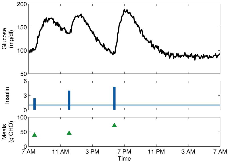
As a proof-of-concept study, a physiological model^10–12 of type 1 diabetes was used to simulate days of normal operation and five realistic faults. The nonlinear model includes dynamics accounting for glucose absorption from meals and subcutaneous-to-intravenous insulin absorption. The simulated normal days included three meals for breakfast, lunch, and dinner, and three corresponding insulin boluses. To simulate realistic, ambulatory conditions, the meal times and amounts (in grams of carbohydrate, or CHO) and insulin bolus times and amounts were randomly chosen from reasonable Gaussian distributions. In addition to the randomness of the meals and boluses, white Gaussian noise^13–15 was added to the glucose concentration measurement. Thirteen days of normal data were simulated, from which ten were used to generate the PCA model (i.e., the training data) and three were retained for use as test data. An example of a normal day is shown in Figure 1.

Figure 1.

Representative normal day for the simulation study. The insulin basal rate (continuous line) is plotted in U/h, while the boluses (bars) are plotted in U.

Three days each of five realistic faults were simulated using the physiological model to determine if the PCA monitoring strategy could distinguish between normal days and faults. Three faults simulated changes in insulin sensitivity (two decreases and one increase); one fault simulated a pump occlusion or kink in the insulin infusion catheter; and the last fault simulated a sensor bias. Table 1 summarizes the datasets used in the analysis.

Table 1.

Simulation conditions.

Type	Number of Runs	Description
NC	10	Normal conditions (training)
NV	3	Normal conditions (testing)
F1	3	Mild decrease in insulin sensitivity (10%)
F2	3	Moderate decrease in insulin sensitivity (25%)
F3	3	Mild increase in insulin sensitivity (10%)
F4	3	Pump occlusion: reduction in basal flow rate (50%)
F5	3	Sensor bias: reduction in glucose measurements (20%)

Three key parameters in the physiological model are related to insulin sensitivity; thus, to simulate changes in insulin sensitivity (faults F₁ − F₃), these parameters were decreased or increased. For the occlusion fault (F₄), the virtual subject was given only half the insulin he or she thought was being delivered. The data used in the PCA, however, corresponded to normal data. The assumption for this fault is that the monitoring system would be unaware of the occlusion, and thus must infer it from the available input-output (i.e., insulin, meal, and glucose) data. For the sensor bias fault (F₅), the glucose measurements were artificially reduced by 20%, simulating a sudden bias in sensor accuracy resulting from, for example, a sensor malfunction.

Ambulatory Subject Data

Nine adult type 1 diabetes subjects (6 women and 3 men) participated in the study, each of whom signed an informed and witnessed consent form approved by the Cottage Health Systems Internal Review Board. The mean (standard deviation) age of the subjects was 38.4 (12.7) years, the body mass index was 23.9 (2.8) kg/m², the hemoglobin A1c was 6.8 (1.0)%, and the duration of diabetes was 19.6 (10.7) years. Subjects were eligible to participate if they had type 1 diabetes without major complications and were using a continuous subcutaneous insulin infusion (CSII) pump. The subjects were trained in the proper use of the CGMS® device (Medtronic MiniMed, Inc., Northridge, CA) and the OneTouch® UltraSmart® blood glucose meter (LifeScan, Inc., Milpitas, CA), and entered at least 4 blood glucose meter values per day into the CGMS for calibration purposes.

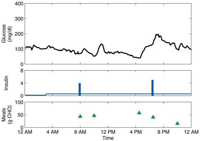
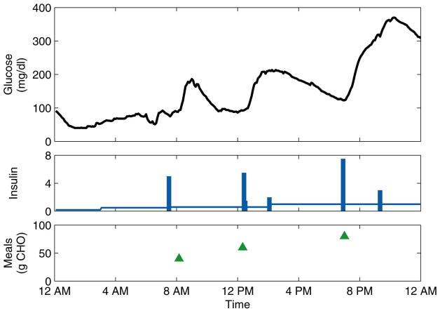
Initially, two to twelve days of data were collected in normal, ambulatory conditions. The data consisted of continuous (5-min) glucose measurements obtained from the CGMS, insulin pump records of basal rates and bolus amounts and times, and subject-recorded estimates of the times and CHO content of meals. PCA models were calculated, on a subject-by-subject basis, from these normal data. All subsequent data were used for model testing. After these first days of normal data, six of the subjects then administered themselves prednisone for three consecutive days, simulating physiological stress by decreasing their sensitivity to insulin. For some subjects, data were collected for days immediately following the stress days, during which the residual effects of the prednisone were largely unknown. These “post-stress” days were not counted in the calculation of the monitoring metrics due to this uncertainty. For all subjects, additional days of normal data were collected. (The three subjects who did not take prednisone were considered “control group” subjects, and their data were used to determine if the PCA models classified the normal test days correctly, a measure of the specificity of the monitoring strategy.) A representative normal day and stress day are shown for one subject in Figure 2 and Figure 3, respectively.

Figure 2.

Representative normal day for Subject 6. The insulin basal rate (continuous line) is plotted in U/h, while the boluses (bars) are plotted in U.

Figure 3.

Representative stress day for Subject 6. The insulin basal rate (continuous line) is plotted in U/h, while the boluses (bars) are plotted in U.

PCA

PCA is a standard statistical technique which finds the directions of greatest variability in multivariate datasets.^16–19 The diabetes datasets in this paper consist of measurements of four variables: blood glucose, insulin basal rate, insulin bolus amount, and meal amount. Consider a dataset X with m rows (observations, or samples) and n columns (variables). This dataset can be expanded as

$$\mathbf{X}={\mathbf{t}}_1{\mathbf{p}}_1^T+{\mathbf{t}}_2{\mathbf{p}}_2^T+\cdots {\mathbf{t}}_k{\mathbf{p}}_k^T+\mathbf{E}=\mathbf{T}{\mathbf{P}}^T+\mathbf{E}$$ (1)

where: P ≡ [p₁ p₂ ··· p_k] is the matrix of n×1 loading vectors (PCs),

T ≡ [t₁ t₂ ··· t_k] is the matrix of m×1 score vectors,

E is the matrix of m × n residuals, and

k is the number of PCs in the model.

There are p_i eigenvectors of Σ, the covariance matrix of X:

$$\mathbf{\sum }=\frac{1}{m-1}{\mathbf{X}}^T\mathbf{X}.$$ (2)

The eigenvalue of Σ associated with the eigenvector p_i is denoted by λ_i. Thus,

$$\mathbf{\sum }{\mathbf{p}}_i={\lambda }_i{\mathbf{p}}_i.$$ (3)

The amount of variance in the dataset X that PC p_i captures is

$$f_{v,i}=\frac{{\lambda }_i}{{\sum }_{j=1}^n{\lambda }_j}i=1,2,\dots ,k.$$ (4)

By definition, the first PC p₁ captures more variance in X than any other PC; therefore its corresponding eigenvalue is λ₁ where the eigenvalues are ordered as

$${\lambda }_1>{\lambda }_2>\cdots >{\lambda }_k>0.$$ (5)

The scores t_i are geometric projections of X onto the PCA model. Thus, to ascertain whether a new (i.e., test) data point x_test is representative of normal operation, it is projected onto the PCA model developed from the training data. Then a score vector t_test for the new data point is calculated as

$${\mathbf{t}}_{\mathit{test}}={\mathbf{x}}_{\mathit{test}}\mathbf{P}$$ (6)

Also calculated for the new data point is a vector of the PCA model residuals:

$${\mathbf{e}}_{\mathit{test}}={\mathbf{x}}_{\mathit{test}}-{\mathbf{t}}_{\mathit{test}}{\mathbf{P}}^T$$ (7)

From these score and model residual vectors associated with the new data point, two statistics known as Q and T² can be calculated and compared to the corresponding statistics for the training data. If the statistics for the new data point violate a reasonable confidence level that describes the training data, say a 95% confidence level, then the new data point is classified as abnormal.

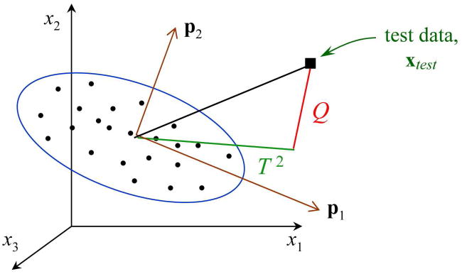
Figure 4 shows a geometric interpretation of the PCA monitoring strategy. In this example, the data consist of measurements of three variables, x₁, x₂, and x₃. The samples used in calculating the PCA model (i.e., the training data) are denoted by dots. Two PCs were retained in the PCA model, p₁ and p₂, which form the plane of the PCA model. The ellipse represents the confidence limits, based on the training data, for the PCA model. A new data point x_test is projected onto the PCA model to determine if it is “similar” to the training data, i.e., if it is described accurately by the PCA model. Two statistics, Q and T², are calculated for the new data point and compared to the corresponding confidence limits for the training data. The Q statistic is the sum of the squared residuals, i.e., $Q={\mathbf{e}}_{\mathit{test}}{\mathbf{e}}_{\mathit{test}}^T$, and thus is related to variability outside the PCA model. The T² statistic describes variability within the PCA model.¹⁹

Figure 4.

Graphical representation of monitoring based on principal component analysis (PCA). Multivariate data consist of measurements of three variables, x₁, x₂, and x₃. Two principal components comprise the PCA model, p₁ and p₂. The Q and T² statistics are shown for a new, test data point x_test.

In the current application of PCA, the X matrix actually consists of three dimensions: samples × variables × days. Thus, this three-dimensional data matrix had to be “unfolded” into two dimensions, where the rows represented days. This technique is known as multiway PCA.¹⁷ For each day, a row for the glucose measurements is listed for the entire day, followed by a row for the basal rates, followed by a row for the boluses, followed by a row for the meals. The training data X consisted only of the first few normal days of data; the test data X_test consisted of all three stress days (if applicable) and at least one normal test day.

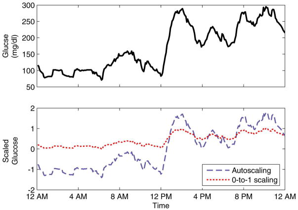
In general, the results of PCA are affected by the manner in which the data are scaled. Scaling in some form is required in this research due to the different orders of magnitude of the measured variables. For example, glucose was measured in mg/dl, for which a physiological range is approximately 40–400 mg/dl, while the basal rate was measured in U/h, for which a reasonable range is approximately 0.5–2 U/h. Two scaling techniques were investigated in this research: autoscaling and “0-to-1” scaling. For autoscaling, the mean and standard deviation are calculated for each variable (e.g., glucose) in the training data. The mean μ is subtracted from each measurement and the result is divided by the standard deviation σ. Thus, for measurements which are normally distributed, autoscaling standardizes the distribution, i.e., N(μ, σ²) is mapped into N(0,1). It should be noted that the data in this research are neither normally distributed nor stationary (i.e., having a constant mean).

In the second scaling method, the data were scaled linearly from 0 to 1. Thus, the minimum value for each variable in the training data was mapped to 0, the maximum to 1, and all data in between were linearly interpolated. It was possible for test data to fall outside the 0-to-1 range, via linear extrapolation. Figure 5 shows a representation of the differences in the scaling methods.

Figure 5.

Comparison of glucose data (top) and scaled data (bottom).

Results and Discussion

Simulation Study

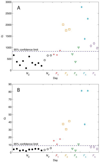
Figure 6(A) shows the PCA monitoring results for the simulation study using the Q statistic and the autoscaled data. The three normal test days, N_V, were classified correctly, thus validating the PCA model developed from the normal training days, N_C. For faults F₁ and F₃, both mild changes in insulin sensitivity, only one of the three days was classified as abnormal based on a 95% confidence limit violation. All three days for the other three faults, F₂, F₄, and F₅, clearly violated the confidence limit, and so were classified correctly. Thus, out of a total of 15 fault days, 11 were classified correctly (73% sensitivity), and all three normal test days were also classified correctly (100% specificity). Because the T² statistic was found to be insensitive to the faults simulated in this study, the results are not shown.

Figure 6.

PCA results for the simulation study using the Q statistic. (A) Autoscaling. (B) 0-to-1 scaling.

Figure 6(B) shows the results for the simulation study using the Q statistic and the 0-to-1 scaled data. Again, the normal test days N_V were classified correctly. All days for faults F₁, F₂, and F₄ were classified correctly, but only one day for F₃ was classified correctly. Fault F₅ went undetected (i.e., classified incorrectly). Thus, 10 of the 15 fault days were classified correctly (67% sensitivity), and all three normal test days were classified correctly (100% specificity). As was the case for the autoscaled data, the T² statistic was found to be insensitive to the faults (results not shown).

Experimental Study

Table 2 summarizes the PCA monitoring results for the experimental data in terms of sensitivity and specificity. Due to the tendency of the T² statistic to be insensitive to faults, a lower confidence limit was investigated for this statistic, namely 75%. This confidence limit may be viewed as a “tuning parameter” if the monitoring strategy were to be implemented in an artificial β-cell. Table 2 shows that, using autoscaled data, the Q statistic is highly sensitive (100%) to the stress days, but only specific about half of the time (47%). In other words, Table 2 indicates that monitoring using autoscaling would tend to identify a high percentage of the stress days correctly, but would produce many “false alarms,” the classification of a normal day as a stress day.

Table 2.

Summary of all experimental results.

		Q (95%)	T2 (75%)
Autoscaling	Sensitivity (%)	100	0
	Specificity (%)	47	100
0-to-1 Scaling	Sensitivity (%)	89	44
	Specificity (%)	89	100

Using 0-to-1 scaling, the Q statistic is both highly sensitive and specific (89% for both metrics). Of 18 stress days, 16 were classified correctly, and of 19 normal test days, 17 were classified correctly. These promising results indicate that monitoring based on the Q statistic with 0-to-1 scaling will result in high sensitivity and specificity levels.

Even for the 75% confidence limits, the T² statistic was still insensitive to the stress days using autoscaling. The sensitivity increased significantly to 44% when using 0-to-1 scaling, but this detection method was unable to detect even half of the stress days.

Table 3 lists the subject-by-subject monitoring results based on the Q statistic. The monitoring method demonstrated consistently accurate results for all subjects, especially when using 0-to-1 scaling.

Table 3.

Subject-by-subject PCA results for the experimental test data using the Q statistic.

Subject ID	Type of Day	Autoscaling		0-to-1 Scaling
		✓	X	✓	X
1	S	3	0	3	0
	N	1	0	1	0
2	S	3	0	3	0
	N	0	1	1	0
3	S	--	--	--	--
	N	0	2	1	1
4	S	--	--	--	--
	N	1	0	1	0
5	S	3	0	2	1
	N	0	3	3	0
6	S	3	0	3	0
	N	1	1	2	0
7	S	3	0	2	1
	N	3	1	3	1
8	S	3	0	3	0
	N	1	1	2	0
9	S	--	--	--	--
	N	2	1	3	0
Total	S	18	0	16	2
	N	9	10	17	2

(S)tress day, (N)ormal day. (✓) correct classification, (X) incorrect classification.

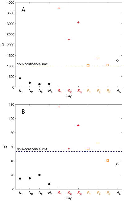
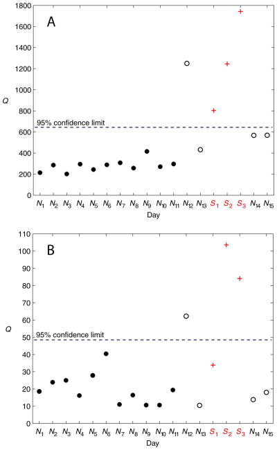
Figures 7 and 8 show PCA monitoring results for two subjects (Subjects 2 and 7, respectively) for the two scaling methods. Figure 7 illustrates the decreased specificity in the monitoring technique using autoscaling (relative to using 0-to-1 scaling), seen by the misclassification of the normal test day N₅. Conversely, Figure 8 illustrates the (slightly) increased sensitivity using autoscaling (again, relative to using 0-to-1 scaling), seen by the correct classification of the stress day S₁.

Figure 7.

PCA results for Subject 2 using the Q statistic. (A) Autoscaling. (B) 0-to-1 scaling. The PCA model was developed from the normal training days N₁ − N₄. All subsequent days are test data. The stress days are denoted by S₁ − S₃. The post-stress days are denoted by P₁ − P₃. Post-stress days are not included in the results due to the unknown residual effects of the prednisone during these days. Day N₅ is a normal test day.

Figure 8.

PCA results for Subject 7 using the Q statistic. (A) Autoscaling. (B) 0-to-1 scaling. The PCA model was developed from the normal training days N₁ − N₁₁. All subsequent days are test data. The stress days are denoted by S₁ − S₃. Days N₁₂ − N₁₅ are normal test days. There were no post-stress days of data collected for this particular subject.

Conclusions

The goal of this research was to determine if a monitoring strategy based on PCA was able to distinguish between normal days of type 1 diabetes data and abnormal days. Several types of abnormal days were investigated in a simulation study, including insulin sensitivity changes, an insulin pump occlusion, and a glucose sensor malfunction. For the type 1 diabetes patients, the abnormal days were days during which physiological stress states were simulated by the administration of prednisone, which served to decrease the subjects’ sensitivity to insulin.

The proposed PCA monitoring technique was capable of distinguishing between the normal days and the abnormal days in both the simulation study and in the data from the diabetes patients. For the experimental data, the monitoring technique exhibited high values for both sensitivity (89%) and specificity (89%). Such an effective monitoring strategy is crucial to the robustness of an artificial β-cell.

References

- 1.Centers for Disease Control and Prevention. National Diabetes Fact Sheet: General Information and National Estimates on Diabetes in the United States, 2007. Atlanta, GA: U.S. Department of Health and Human Services, Centers for Disease Control and Prevention; 2008. [Google Scholar]
- 2.Ashcroft FM, Ashcroft SJH. Insulin: Molecular Biology to Pathology. Oxford University Press; New York, NY: 1992. [Google Scholar]
- 3.Finan DA. PhD Thesis. University of California; Santa Barbara: 2008. Modeling and Monitoring Strategies for Type 1 Diabetes. [Google Scholar]
- 4.Parker RS, Doyle FJ, III, Peppas NA. A Model-based Algorithm for Blood Glucose Control in Type 1 Diabetic Patients. IEEE Trans Biomed Eng. 1999;46(2):148–157. doi: 10.1109/10.740877. [DOI] [PubMed] [Google Scholar]
- 5.Bellazzi R, Siviero C, Stefanelli M, De Nicolao G. Adaptive Controllers for Intelligent Monitoring. Artif Intell Med. 1995;7:515–540. doi: 10.1016/0933-3657(95)00025-x. [DOI] [PubMed] [Google Scholar]
- 6.Bevier WC, Zisser H, Jovanovic L, Finan DA, Palerm CC, Seborg DE, Doyle FJ., III Use of Continuous Glucose Monitoring to Estimate Insulin Requirements in Patients with Type 1 Diabetes Mellitus During a Short Course of Prednisone. J Diabetes Sci Technol. 2008;2(4):578–583. doi: 10.1177/193229680800200408. [DOI] [PMC free article] [PubMed] [Google Scholar]
- 7.Bequette BW. A Critical Assessment of Algorithms and Challenges in the Development of a Closed-loop Artificial Pancreas. Diabetes Technol Ther. 2005;7(1):28–47. doi: 10.1089/dia.2005.7.28. [DOI] [PubMed] [Google Scholar]
- 8.Hovorka R. Management of Diabetes Using Adaptive Control. Int J Adapt Control Signal Process. 2005;19:309–325. [Google Scholar]
- 9.Finan DA, Zisser H, Jovanovic L, Bevier WC, Seborg DE. Identification of Linear Dynamic Models for Type 1 Diabetes: A Simulation Study. Proc IFAC ADCHEM Sympos. 2006:503–508. [Google Scholar]
- 10.Hovorka R, Shojaee-Moradie F, Carroll PV, Chassin LJ, Gowrie IJ, Jackson NC, Tudor RS, Umpleby AM, Jones RH. Partitioning Glucose Distribution/Transport, Disposal, and Endogenous Production During IVGTT. Am J Physiol Endocrinol Metab. 2002;282:992–1007. doi: 10.1152/ajpendo.00304.2001. [DOI] [PubMed] [Google Scholar]
- 11.Hovorka R, Canonico V, Chassin LJ, Haueter U, Massi-Benedetti M, Federici MO, Pieber TR, Schaller HC, Schaupp L, Vering T, Wilinska ME. Nonlinear Model Predictive Control of Glucose Concentration in Subjects with Type 1 Diabetes. Physiol Meas. 2004;25:905–920. doi: 10.1088/0967-3334/25/4/010. [DOI] [PubMed] [Google Scholar]
- 12.Wilinska ME, Chassin LJ, Schaller HC, Schaupp L, Pieber TR, Hovorka R. Insulin Kinetics in Type–1 Diabetes: Continuous and Bolus Delivery of Rapid Acting Insulin. IEEE Trans Biomed Eng. 2005;52:3–12. doi: 10.1109/TBME.2004.839639. [DOI] [PubMed] [Google Scholar]
- 13.Mastrototaro JJ. The MiniMed Continuous Glucose Monitoring System. Diabetes Technol Ther. 2000;2(Suppl 1):S13–18. doi: 10.1089/15209150050214078. [DOI] [PubMed] [Google Scholar]
- 14.Florian JA, Jr, Parker RS. Empirical Modeling for Glucose Control in Critical Care and Diabetes. Eur J Control. 2005;11:601–616. [Google Scholar]
- 15.Finan DA, Zisser H, Jovanovic L, Bevier WC, Seborg DE. Practical Issues in the Identification of Empirical Models from Simulated Type 1 Diabetes Data. Diabetes Technol Ther. 2007;9:438–450. doi: 10.1089/dia.2007.0202. [DOI] [PubMed] [Google Scholar]
- 16.Jolliffe IT. Principal Component Analysis. 2. Springer; New York, NY: 2002. [Google Scholar]
- 17.Nomikos P, MacGregor JF. Multivariate SPC Charts for Monitoring Batch Processes. Technometrics. 1995;37(1):41–59. [Google Scholar]
- 18.Chiang LH, Russell EL, Braatz RD. Fault Detection and Diagnosis in Industrial Systems. Springer-Verlag London Limited; Great Britian: 2001. [Google Scholar]
- 19.Wise BM, Gallagher NB, Bro R, Shaver JM. MATLAB PLS Toolbox 3.0 Manual. Eigenvector Research, Inc; Manson (WA): 2003. [Google Scholar]