Classification of Mycobacterium tuberculosis in Images of ZN-Stained Sputum Smears

Abstract

Screening for tuberculosis (TB) in low- and middle-income countries is centered on the microscope. We present methods for the automated identification of Mycobacterium tuberculosis in images of Ziehl–Neelsen (ZN) stained sputum smears obtained using a bright-field microscope. We segment candidate bacillus objects using a combination of two-class pixel classifiers. The algorithm produces results that agree well with manual segmentations, as judged by the Hausdorff distance and the modified Williams index. The extraction of geometric-transformation-invariant features and optimization of the feature set by feature subset selection and Fisher transformation follow. Finally, different two-class object classifiers are compared. The sensitivity and specificity of all tested classifiers is above 95% for the identification of bacillus objects represented by Fisher-transformed features. Our results may be used to reduce technician involvement in screening for TB, and would be particularly useful in laboratories in countries with a high burden of TB, where, typically, ZN rather than auramine staining of sputum smears is the method of choice.

I. Introduction

The microscope is at the heart of tuberculosis (TB) screening, particularly in low-income countries [1]. Positive sputum smear detection by microscopy makes up the largest fraction of TB detections, according to the World Health Organization (WHO) [2].

A major shortcoming of TB screening with a conventional microscope is that sensitivity is variable: values between 20% and 60% have been reported in some studies, while sensitivity above 80% has been reported in others [1]. Some research efforts have been directed at specimen preparation techniques that improve sensitivity, at the cost of specificity [3]. Technicians may diagnose a positive TB slide as smear negative because of sparseness of acid-fast bacilli, or because too few fields have been examined.

A fluorescence microscope is used to examine auramine-stained sputum smears, while a bright-field microscope is used to examine Ziehl–Neelsen (ZN) stained sputum; fluorescence microscopy is on average 10% more sensitive than bright-field microscopy in detecting TB in sputum smears [1]. We concentrate on TB screening using bright-field microscopy of ZN-stained sputum smears, as this is the method of choice in developing countries, due to the low cost and ease of equipment maintenance compared to fluorescence microscopy; low-cost fluorescence microscopes have, however, recently become available [4]. Fig. 1 shows an example ZN-stained sputum smear image.

Fig. 1.

Example ZN-stained sputum smear image.

The aim of automation in the context of TB screening is to speed up the screening process and to reduce its reliance on technicians and pathologists. The demands on technicians in high-prevalence countries lead to overload and fatigue, which diminish the quality of microscopy [5]. There is a shortage of senior pathologists to verify manual screening—as stipulated by the WHO—in developing countries. Automation may also improve the low sensitivity of conventional TB screening by microscopy and reduce human variability in slide analysis.

Veropoulos et al. [6] and Forero et al. [7] were the first to propose pattern recognition techniques for the identification of TB in images of auramine-stained sputum smears. Canny edge detection has been used to segment TB bacilli in captured images [6], [8]–[10]. Edge pixel linkage [6] and morphological closing [8]–[10] have been applied to segmented objects to complete broken edge contours. Forero et al. [7] used fuzzy thresholding to segment images of sputum smears. Edge detection techniques perform poorly on images of ZN-stained sputum smears because such images have greater background variability than auramine-stained images from a fluorescence microscope.

The literature shows a trend in using classifiers to segment objects from microscope images [11]–[16]. Support vector machines (SVMs) were used in [15] to quantify the amount of Mycobacterium tuberculosis in confocal microscopy images for drug discovery. Santiago-Mozos et al. [16] used pixel classification to detect bacilli in fluorescence images of auramine-stained sputum; each pixel was represented by a square patch of its neighbors.

Pixel classifiers hold promise for the segmentation of bacilli from ZN-stained sputum smear images [17], because of their ability to exploit the color differences between bacilli and background in these images. The red color of the ZN carbol fuchsin stain is absorbed by the waxy coating of bacilli during staining, while the background is stained blue with a methylene blue counterstain.

The advantages of pixel classifiers over edge detection for the segmentation of bacilli in images of ZN-stained sputum are that they respond better to the background variability of ZN-stained images, and that they are less likely to miss objects with poorly defined edges. Their performance is improved by considering the relative distributions of object classes in captured images. The biggest drawback of pixel classifiers is that they do not consider spatial information. We combine individual classifiers to improve performance.

Veropoulos et al. [6] used Fourier descriptors to classify segmented objects as either bacillus or nonbacillus; they used a feedforward neural network with four hidden units for classification. Hu’s moments were used in [9] and [10] to describe segmented candidate bacillus objects, and k-means clustering and a minimum error Bayesian classifier were used for classification [10]. The classifier was unsupervised; it had clustered data as input. These earlier methods were applied to images from a fluorescence microscope. Sadaphal et al. [11] demonstrated color-based Bayesian segmentation of TB bacilli in images of ZN-stained sputum smears. We have previously used one-class classifiers for pixel and object classification in sputum smear images [17].

This paper presents a combination of pixel classifiers for image segmentation to extract candidate bacillus objects from images of ZN-stained sputum smears. The extraction of features that describe segmented objects follows. The most descriptive features are then selected, and the final step in the bacillus detection process is the classification of objects as bacilli or nonbacilli. We use a feature mapping algorithm to enhance the separability between the two classes. The results of segmentation and classification are validated quantitatively.

II. Materials and Methods

A. Image Acquisition

Images were taken using a Nikon Microphot-FX microscope with a 100× oil objective and 1.4 numerical aperture. Attached to the microscope was a Kodak DC290zoom digital camera. The pixel resolution was 720 × 480. The images were stored in JPEG file format, with 24 bits per pixel, in color.

To standardize images, Kohler illumination was applied once and fixed for all slides. White balance was performed for each slide. The microscope was used without any filters, and its 12-V, 100-W halogen lamp was set to 7–9 V. The images were captured in a room lit by a fluorescent light. The camera zoom was set at 65 mm and exposure time at 0.1 s.

Sputum smear slides were prepared by the South African National Health Laboratory Services (NHLS) at Groote Schuur Hospital in Cape Town, South Africa. Nineteen smear-positive slides from 19 different subjects were used. The slides did not have cover slips, and between 20 and 100 images were taken per slide.

B. Segmentation

We use pixel classifiers to segment images of ZN-stained sputum smears. We combine a number of classifiers to produce better segmentation than using pixel classifiers individually. A combination of pixel classifiers was found to be superior to individual pixel classifiers to segment microscope images for lung cancer diagnosis [13].

1) Pixel Classifiers

The Bayes’ classifier minimizes the probability of error in assigning a class to an object. An object is assigned a class whose probability density function dominates at its position [18].

The linear regression classifier finds a linear mapping between stored points and their labels, and uses the mapping to predict labels of query points. The mapping minimizes the errors between classes in the least square sense, using the Euclidean distance. The logistic linear classifier is obtained by iteratively reweighting the least squares solution to the plot of a line separating the two classes [19].

The quadratic discriminant classifier is similar to the linear regression classifier. The training data points are used to establish a quadratic mapping between objects and their labels. The discrimination is drawn using the class mean and covariance matrices [19].

For all pixel classifiers, the input was the captured RGB image, and the output was the logical image used to index segmented objects for feature extraction. Extracted features formed a dataset for input to object classifiers.

2) Classifier Training

Image pixels were used as objects. The dataset of images used to train pixel classifiers was derived from nine subjects and was composed of 28 images, from which pixels of bacilli in the focal plane were labeled as +1. A subset of background pixels was labeled as −1. The dataset contained 40 666 objects, of which 20 637 were bacillus objects.

Bayes’ classifier was trained by estimating the mean and covariance matrices of the two classes in the training dataset. Training of the logistic and Euclidean linear classifiers involved establishing the mapping that classifiers used to label objects of the training dataset. Lastly, the quadratic classifier used the training dataset to find the covariance matrices of the two classes.

3) Combination Schemes

The classifiers were assessed using a dataset of five images from different subjects. Each of the images had a manually segmented version used to validate the segmentation results.

Classifiers were combined using different combination schemes and the segmentation performance of each combination was evaluated. The combination schemes used were the mean, median, minimum, maximum, and the product of classifiers’ output posterior probabilities [13]. All classifiers assigned two posterior probabilities to a pixel, one for each class, namely bacillus and nonbacillus. A pixel assumed the label of the class with the highest probability.

4) Segmentation Validation

Segmentation was validated using the procedure proposed in [14]. A manually segmented reference image was used to provide true or false classification rates. To compute these rates, the common and difference rates are found. The common rate is the number of pixels belonging to objects that are correctly classified and the difference rate is the number of pixels that belong to objects in the reference image but are not identified as the same class in the segmented image and pixels that belong to background in the reference image identified as object pixels in the segmented image. For each class, the common rate is averaged by object pixels in the reference image to give the percentage of correctly classified pixels. The difference rate is averaged by the union of the reference image object pixels and the segmented image object pixels to give the percentage of incorrectly classified pixels. This evaluation procedure was used to select the best combination scheme for segmentation to produce objects from which features may be extracted to classify objects as either bacillus or nonbacillus.

Since manually segmented objects were used as the gold standard in comparing classifiers, the agreement of manual segmentations with segmentations produced by the best combination of pixel classifiers was assessed using the Hausdorff distance [20] and the modified Williams index (MWI) [21].

C. Feature Extraction

The 2-D coordinates of the boundary pixels of an object form a closed shape. Starting at an arbitrary point, the boundary can be represented as a complex sequence of coordinates. The second value of each coordinate s(k) is made imaginary, for k = 0, 1, 2, …, K − 1, where K is the number of boundary pixels. The discrete Fourier transform of s(k) is given by

$$a(u)=\sum _1^{K-1}s(k)e^{(-j\pi 2uk/K)}.$$ (1)

The complex coefficients a(u), u = 0, 1, 2, …, K − 1, can be used as Fourier features [22]. Fourier features can be made invariant to translation and rotation using the transform: $r(u)=\sqrt{{\mid a_x(u)\mid }^2+{\mid a_y(u)\mid }^2}$, where a_x (u) and a_y (u) are the real and imaginary parts of the coefficients or descriptors. The classification accuracy of the nearest-neighbor (NN) classifier was used to determine the number of coefficients to use.

Fourier features are geometric-change invariant, as are moment invariant features. Moment features are derived from the generalized color moment [23]. For an RGB image, the generalized color moment is

$$M_{pq}^{\mathit{abc}}=\int {\int }_{\mathrm{\Omega }}{x}^p{y}^q{[R(x,y)]}^a{[G(x,y)]}^b{[B(x,y)]}^{c}dxdy$$ (2)

where p + q is the order and a + b + c the degree. The moment invariants derived from the generalized color moment have degree confined to two.

The eccentricity of an object is the ratio of its major and minor axes. Compactness provides a measure of how closely the shape of the object approaches a circle, and it is the ratio of the perimeter and area of the object. Eccentricity and compactness capture the long and thin shape of bacilli.

For each color channel, the value of the central pixel was considered as a feature, as were the mean of all and of the perimeter pixel values. The last two color features were the standard deviations of all and of the perimeter pixel values. The features were normalized so that no feature would dominate in the decision making of the classifier, by subtracting the mean of each feature from each feature element, then dividing each feature element by the standard deviation of that feature. The most descriptive set of features was selected from the normalized features.

D. Feature Subset Selection

Several feature selection algorithms were implemented. Population-based incremental learning (PBIL) selects feature subsets probabilistically. The search is progressively prejudiced toward subsets that yield a higher evaluation figure of merit by using weights [24].

The correlation-based feature selection (CFS) algorithm evaluates features using

$$\text{Merit}=\frac{{kr}_{rc}}{\sqrt{k+k(k-1)r_{ff}}}$$ (3)

where r_{r c} is the average feature–class correlation and r_ff is the average feature–feature correlation for a subset with k features. The dot product of two vectors can be interpreted as their correlation and reveals the directional relationships of the two vectors. It is usually normalized by the magnitudes of the two vectors to the range −1 to +1. The evaluation function selects features to a subset that are uncorrelated to current features in a subset, yet highly correlated to the class vector [25].

Sequential floating forward or backward selection (SFFS or SBFS) performs a fixed number of F steps forward or backward to find the next best feature. This is done until a desired number of features is obtained. After inclusion of each feature, backtracking is applied to observe if removing any of the present features increases an evaluation figure of merit [26].

Branch and bound (B&B) feature selection uses an evaluation function to select the best subset of d features out of M features. It models the tree, where the root is the set of all features and the leaves are subsets with d features. The evaluation function is used to follow a path with the highest evaluation. This path leads to the best subset. According to Somol et al. [27], it is an optimal feature selection algorithm in that it cannot miss the best subset of features.

All the feature subset selection algorithms, except CFS, used the classification accuracy of the NN classifier as an evaluation figure of merit.

E. Feature Dimensionality Reduction

Scatter matrices are class separability criteria based on the manner in which feature vectors are scattered in the feature space. Fisher mapping reduces the dimensionality of the feature space based on the optimization of the between-class scatter matrix S_b with respect to the within-class scatter matrix S_w [28]:

$$\begin{array}{l}{S}_b={\sum }_{i=1}^m{N}_i(u_i-u_o){(u_i-u_o)}^T\\ S_w={\sum }_{i=1}^m\sum _{x_k\in X_i}{N}_i(x_k-u_i){(u_k-u_i)}^T.\end{array}$$ (4)

For each of the m classes, N_i is the number of samples in class X_i, u_i is the mean of class X_i, and u_o is the global mean vector. The optimal projection maximizes the determinant of S_b with respect to that of S_w.

The Fisher transformation was applied to the extracted features as an alternative to feature subset selection for optimization of the feature set prior to classification.

F. Object Classification

The last step in the bacillus identification process is the classification of segmented objects. Using the selected subset of features, we compared the Bayes’, linear, quadratic, and kNN classifiers, as well as probabilistic neural networks (PNNs) and SVMs. The first three classifiers are described in Section II-B.

The NN classifier predicts the labels of query objects by comparing them to stored objects whose labels are known [18]. The Euclidean distance between each query point and the stored points is used for comparison. If k points are used instead, NN extends to kNN. Greene [29] proposes the use of the Thornton separability index (SI) to determine the generalization performance of the kNN classifier, in order to avoid evaluation by multiple data splits into train-test sets. SI can be used to determine the value of k to be used in the kNN classifier.

Single-layered radial basis function (RBF) networks are appealing because they are easier to train than multilayered perceptron (MLP) neural networks [18]. Their single hidden layer is composed of RBFs, and Gaussians are frequently used. The output layer of an RBF network is a linear transformation of the outputs of RBFs. It can be optimized using linear techniques that are faster than MLP training techniques. PNNs are RBF networks used for classification [18]. The PNN classifier has one tuning parameter, the kernel width parameter, and leave-one-out validation can be used to search for its optimum.

SVMs [30] select a hyperplane that maximizes the margin between two classes, where the margin represents the sum of the distances of the hyperplane to the closest points of the two classes, and at the same time the number of classification errors is minimized. SVMs avoid several problems associated with artificial neural networks, for example, they control overfitting by restricting the capacity of the classifier and they depend on the solution of a quadratic programming (QP) problem without local extrema [12]. Training of SVMs involves the search for a positive constant parameter introduced to control the cost of misclassified objects and the parameter of a kernel function. Leave-one-out cross-validation error can be estimated by finding the fraction of support vectors that are correctly classified [31].

The classification results were evaluated using sensitivity, specificity, and accuracy.

III. Results

A. Segmentation

The objects of the training dataset had three features—the pixel values of the three channels of the RGB color space.

Table I shows the ratios of correctly and incorrectly classified pixels for individual classifiers. Fig. 2 shows the percentage of correctly classified pixels for different classifier combinations with increasing number of classifiers. Additional classifiers were added in decreasing order of their individual performance; thus, the first combination consists of the Bayes’ and quadratic classifiers.

TABLE I.

Performance of Pixel Classifiers (For Each Classifier, the First Entry is the Ratio of Correctly Classified Pixels, and the Second Entry is the Ratio of Incorrectly Classified Pixels)

Classifier	Bayes	Euclidean distance linear	Logistic linear	Quadratic
	0.8839	0.8573	0.8770	0.8839
	0.3808	0.3733	0.4259	0.3808

Fig. 2.

Percentage of correctly classified pixels for different numbers of combined classifiers, added in decreasing order of performance.

For the first two classifiers, all combination schemes had the percentage of correctly classified pixels as 88.38%, and had the lowest percentage of incorrectly classified pixels, namely 38.08%. The product of the Bayes’, quadratic, and logistic linear classifiers produced a percentages of correctly and incorrectly classified pixels of 89.38% and 39.52%, respectively. Visual inspection of the segmentation results showed that incorrectly classified pixels often occurred at bacillus boundaries without influencing the shape of the segmented object; for this reason, the classifier combination with the highest percentage of correctly classified pixels was chosen and the increased percentage of incorrectly classified pixels regarded as negligible. The increased number of classifiers incurs negligible computational cost. Examples of segmentation results are shown in Fig. 3.

Fig. 3.

Subimages of the results obtained using the product of classifiers overlaid on two images of the test dataset.

A set of 50 bacilli in 20 images was used to study the agreement of contours segmented by two trained researchers under the guidance of a pathologist and by the algorithm. Objects segmented by the algorithm were visually evaluated and manual comparisons were made for those objects that were bacilli in the focal plane of the image. The comparisons in Table II were made using the Hausdorff distance [20]. T11 and T12 represent the first observer outlining bacilli the first and second times, more than 24 h apart, T2 represents the second observer, and AL represents segmentation using pixel classification. Fig. 4 compares segmentations for which the Hausdorff distances between manual and algorithm segmentations were relatively large.

TABLE II.

Comparison of Manual Segmentation and Segmentation by the Combination of Pixel Classifiers Using the Hausdorff Distance (Units are in Pixels); Std: Standard Deviation (The Contours of 50 Bacilli Were Compared)

	T11 & T12	T21 & T22	T11 & T21	T11 & AL	T21 & AL
Mean	3.8801	2.8894	3.0589	3.4941	4.0955
Std	1.6391	1.3328	1.3595	1.7058	2.0453

Fig. 4.

Examples of manual and algorithm segmentation results and associated Hausdorff distances (HDs); image sizes are 22× 54 and 18× 49 pixels, respectively. The contours of 50 bacilli were compared.

The Hausdorff distance was used to obtain the MWI [21] for comparing computer-generated bacillus boundaries with hand-drawn ones. The index comprises the ratio between the average computer–observer agreement and the average observer–observer agreement. If N is the number of observations, the MWI is calculated leaving one observation out at a time, for N −1 observations, resulting in N estimates. The set of manual segmentations comprised four observations per object: two researchers each outlined the objects twice. The value of the MWI was 0.9602; its 95% confidence interval, assuming the standard normal distribution, was (0.9530, 0.9674). These results indicate that the segmentation boundaries produced by the algorithm agree with manual segmentations almost as well as different manual segmentations agree with one another.

B. Feature Subset Selection

The results of the feature subset selection methods applied to the normalized features are summarized in Table III. The dataset was drawn from 185 segmented images and constituted 1629 bacillus objects and 1697 nonbacillus objects.

TABLE III.

Features Selected by Different Selection Methods

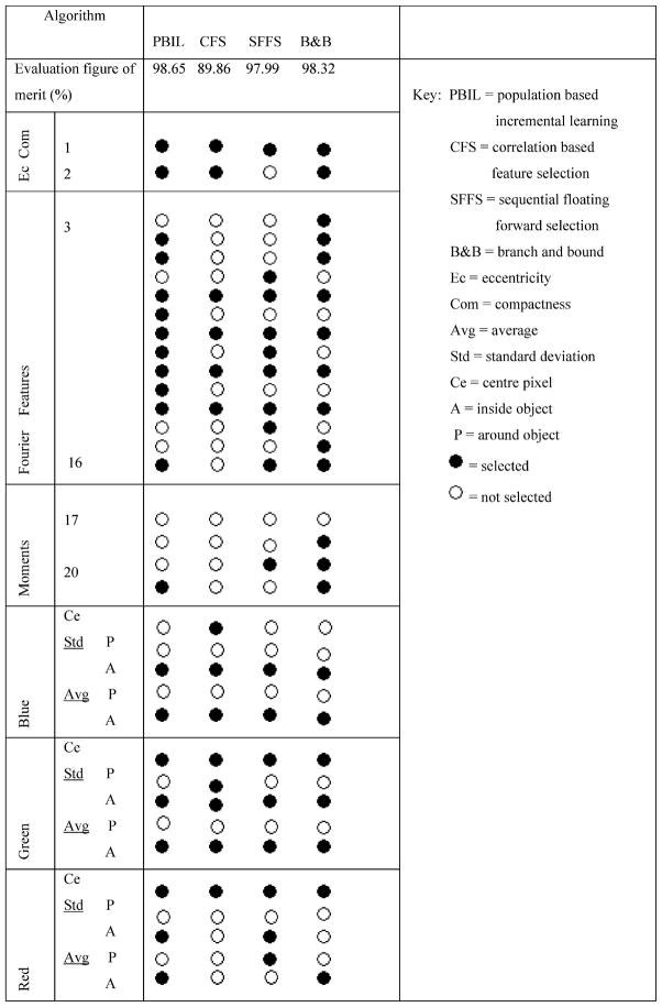C. Object Classification

The training dataset consisted of 6901 objects from 11 subjects. A total of 4999 objects were labeled as bacilli and 1902 were labeled as nonbacilli. The fraction of objects in each class reflects the estimate of the ratio of the objects in each class to the total number objects that the segmentation method yields. Leave-one-out cross-validation was used to train the kNN, PNN, and SVM classifiers. The rest were trained similarly to the pixel classifiers.

Individual bacilli in the focal plane of the image were labeled as bacilli; objects that were clearly not bacilli, such as red stains, as well as touching bacilli, were labeled as nonbacillus objects. Bacilli out of the focal plane of the image were not included in the analysis.

All classifiers were tested using a dataset from eight subjects, with 1838 objects labeled as bacilli and 2520 objects labeled as nonbacilli. Fig. 5 shows shapes of example bacillus and non-bacillus objects.

Fig. 5.

Example bacillus and nonbacillus objects.

The performance of different classifiers with different feature selection procedures, all evaluated at their best operating point as found by cross-validation, is shown in Table IV. Table V shows the performance of classifiers on the Fisher mapping of the full feature set.

TABLE IV.

Performance of Each Classifier at Its Best Operating Point as Found by Cross-Validation

Selection of features	Classifier		Accuracy (%)
			Sensitivity (%)
			Specificity (%)
	kNN	Bayes	Linear	Quad	PNN	SVM
PBIL	88.96	68.24	83.23	76.96	81.02	79.33
	99.13	99.67	99.89	100	99.51	99.13
	81.54	45.32	71.07	60.59	74.44	64.88
B&B	84.47	66.82	82.31	76.07	82.35	77.56
	99.67	99.46	99.73	99.95	99.62	99.29
	73.37	43.02	69.60	58.65	69.76	61.71
CFS	84.37	87.93	83.23	86.85	82.42	80.56
	99.56	99.67	100	99.51	99.40	99.84
	73.29	79.36	70.99	77.62	70.04	66.51
SFFS	87.20	89.01	83.25	75.65	84.83	80.45
	99.62	99.62	99.95	100	99.29	99.51
	78.13	81.27	71.07	57.90	74.29	66.55

TABLE V.

Performance of Classifiers on the Fisher-Mapped Feature Set

	Classifier		Accuracy (%)
			Sensitivity (%)
			Specificity (%)
	kNN	Bayes	Linear	Quad	PNN	SVM
Fisher	98.55	97.67	98.51	97.67	98.53	98.55
mapped	97.77	95.32	97.66	95.32	97.71	97.67
features	99.13	99.37	99.13	99.37	99.13	99.13

IV. Discussion

The aim of our study was to detect TB bacilli in ZN-stained sputum smears, using an algorithm comprising segmentation of candidate bacillus objects and classification of segmented objects.

No evaluation of ZN-stained sputum smear image segmentation was found in the literature for direct comparison with our results. Sadaphal et al. [11] segmented ZN-stained sputum smear images, but did not provide quantitative results. They extracted two shape descriptors from the objects, axis ratio, and eccentricity, and thresholded them to find a range for TB bacilli. Meuric et al. [14] used pixel ratios to assess performance of a combination of classifiers to segment lung cancer images, and obtained satisfactory results. Santiago-Mozos et al. [16] classified patches of pixels in auramine images as either bacillus-containing or not, and they performed sequential tests on detected patches until set false alarm and detection probabilities were met.

The product of three-pixel classifiers produces the best segmentation, as judged by the ratio of correctly classified pixels. No bacillus objects were missed in the focal plane of an image. A theoretical framework and analysis of classifier combination schemes is presented in [32]: improved results are attributed to the possibility of different classifier designs offering complementary information about the patterns to be classified. Using different feature sets for the different classifiers being combined may further improve classification results. A classifier combination for segmentation of candidate bacillus objects based on different color spaces could be considered in future work.

The combined pixel classification algorithm produces segmentation results that agree with manual results almost as often as manual segmentations agree with each other. Fig. 4 shows that the manual and algorithm segmentations associated with larger Hausdorff distances are visually similar and that the features used in classification, namely shape and color, are preserved by both methods. Because segmentation is an intermediate stage in the identification process and influences the classifier results, segmentation algorithms would best be evaluated by comparison of the results of object classification performed on segmented objects produced by different algorithms. However, different segmentation methods produce different segmented objects, and a direct comparison of object classification results to evaluate segmentation is therefore not possible.

The biggest source of error for the segmentation method was red stain deposits that had crystallized, on some slides, possibly due to the delay in washing off the ZN carbol fuchsin with the acid alcohol used to decolorize the slide. One way to eliminate this problem would be automation of the staining procedure, which would further speed up TB screening. Automated staining, or consistency in the staining method, would also allow the methods described here to be applied to datasets obtained in different laboratories, without changes in parameters. The extent to which differences in laboratory practice and the resulting variation in slide features affect the accuracy of bacillus segmentation and classification should be investigated, as should the performance of the algorithm on images from different microscope configurations.

A drawback of our segmentation method is that we used equal priors for both classes in classifier training. It would not, however, be possible, in practice, to predict the relative distribution of bacilli and background pixels in images.

Pixel classifiers segmented fewer nonbacillus objects than would have been produced by conventional low-level image processing techniques such as edge detection. This was the motivation for using the number of objects in each of the two classes defined as priors in object classification. Objects presented to the classifiers for the final identification step were more likely to be bacilli than nonbacilli.

As shown in Table III, the performance of the feature subset selection method appears to be related to the size of the subset of Fourier descriptors. This result highlights the significance of Fourier descriptors in representing shape features.

The 5th, 7th, 9th, and 11th Fourier coefficients were chosen by all feature subset selection methods. The Fourier coefficients chosen most frequently were the central ones. Compactness, which expresses the characteristic rod-like shape of bacilli, is also selected by all methods.

The color features chosen by all feature subset selection methods were the mean and standard deviation of object pixel intensities for the blue and green channels. For the red and green channels, the central pixel value was always chosen. A large portion of misclassified objects had the correct color features, indicating that shape features were more influential in object classification.

With the exception of the CFS algorithm, all feature selection algorithms used a NN-based evaluation function. The good performance of the kNN classifier, as shown in Table III, may, therefore, be expected, as the same inductive method was used for feature selection as for classification [33].

All classifiers performed better on Fisher-mapped features than on subsets of selected features. Fisher mapping was responsible for improved specificity; it pronounced the separability of the two classes. Classifier performance on the Fisher-mapped feature set was balanced, namely sensitivity and specificity were above 95% for the detection of an individual object. Bayes’ and quadratic classifiers had the lowest accuracy of 97.67%.

Veropoulos et al. [6] achieved sensitivity of 94.1% and specificity of 97.4% in the classification of objects in auramine-stained sputum smears (63× magnification) using a feedforward neural network with four hidden units. Thus, our results on ZN-stained sputum are comparable with those reported for auramine-stained sputum, while technicians perform more poorly on ZN-stained smears [1]. Differences in magnification may influence classification accuracy. Forero et al. [10] obtained sensitivity of 97.89% and specificity of 94.67% using a minimum error Bayesian classifier; they calculated accuracies per image (25× magnification) and not per object, thus a direct comparison with bacillus detection is not possible. Our results are also an improvement on those obtained previously using one-class pixel and object classification in ZN-stained smears [17].

Identification may improved by implementing an object filter based on feature values. Objects may be rejected by studying the distribution of each feature and setting thresholds on each. Objects with feature values above a threshold may be declared bacillus objects right away, and only objects with feature values in a specified band sent to the final classification stage.

Future work will include the search for the most descriptive bacillus feature, as simple classifiers may be expected to have good performance with it. Furthermore, there is a need for a feature that will describe touching bacilli, which usually form a T shape. Fig. 6 illustrates the touching bacilli that may be captured with such a feature. The current scheme labels touching bacilli as nonbacilli.

Fig. 6.

Results of the established identification route on an example image; bacillus objects are lighter (red in online version) and nonbacillus objects are darker (blue in online version) in the bottom image; touching bacilli are labeled as nonbacilli.

The classification results presented are based on the distribution of objects in the training dataset. The results may be generalized to a larger population of objects if the properties of the larger set are similar to those of the training set used here, i.e., if proper sampling of the training can be assumed. The assumed prior distribution of the two classes may be verified by determining if, for images from a large set of sputum slides, the segmentation method would yield the same ratio of positive to negative objects as obtained in this study.

V. Conclusion

An automated identification path has been established for M. tuberculosis in images of ZN-stained sputum smears. We report quantitative evaluation of segmentation and classification results for bacilli in ZN-stained sputum smear images. We have found classification accuracies of bacilli in images of ZN-stained sputum smears similar to those reported for auramine-stained sputum smears. The method may be incorporated into an automated microscope for TB detection, which would also feature automatic focusing and stage control. Automated TB microscopy has potential for use in countries with a high TB burden to relieve the shortage of trained technicians.

Biographies

Rethabile Khutlang received the B.Sc. degree in electrical engineering in 2006 and the M.Sc. degree in biomedical engineering in 2009, both from the University of Cape Town (UCT), Cape Town, South Africa.

He is currently with the UCT. His current research interests include image segmentation and classification for automated microscopy, in particular for tuberculosis detection.

Sriram Krishnan received the M.S. degree in electrical engineering from Rensselaer Polytechnic Institute, Troy, NY, in 1993.

He was engaged in several research and development laboratories, including Philips Research Laboratories in Briarcliff Manor, NY, and Bangalore, India, as well as at Analog Devices, Wilmington, MA. He is currently the Project Manager for the automated TB microscopy project at the University of Cape Town, Cape Town, South Africa. His current research interests include signal and image processing, communication systems, applied optics, and systems engineering.

Ronald Dendere received the B.Eng. degree in electronic engineering from the National University of Science and Technology, Bulawayo, Zimbabwe, in 2006, and the M.Sc. degree in biomedical engineering from the University of Cape Town (UCT), Cape town, South Africa, in 2009.

He is currently with the UCT. His current research interests include autofocusing and image processing for microscopy applications.

Andrew Whitelaw received the undergraduate medical training from the University of the Witwatersrand, Johannesburg, South Africa, and the M.Sc. degree in medical microbiology from the University of Cape Town (UCT), Cape Town, South Africa, in 1999.

Since 2003, he has been a Specialist Microbiologist with the National Health Laboratory Service at Groote Schuur and Red Cross Children’s Hospitals, UCT, where he is also a Lecturer. His current research interests include the epidemiology and the laboratory diagnosis of tuberculosis.

Konstantinos Veropoulos received the B.Sc. degree in computer science and engineering from the American University of Athens, Athens, Greece, the M.Sc. degree in parallel computer systems from the University of the West of England, Bristol, U.K., and the Ph.D. degree in machine learning and machine vision from the University of Bristol, Bristol.

He is a researcher in the theory and applications of artificial neural networks and support vector machines and was engaged in machine learning approaches applied to medical, biometric, and atmospheric science applications. He is currently the Environment, Health and Safety Specialist of General Electric (GE) Healthcare, Medical Systems Hellas. He was an External Computer Research Consultant for a number of companies and institutions, including the University of Nevada Reno, the Desert Research Institute, Interscopic Analysis LCC, and the University of Cape Town. He is currently an External Computer Research Consultant with the Guardian Technologies International, Inc., Herndon, VA.

Genevieve Learmonth joined the Department of Anatomical Pathology, University of Cape Town, in 1977, having completed initial training in pathology in Galway and Dublin, and in London at Guys Hospital, National Heart Hospital and Hammersmith Hospital. She qualified as a Specialist Histopathologist in Cape Town, focusing on cytopathology and population screening for the identification and treatment of women who are at risk of developing cervical cancer, in South Africa. She has been involved in the evolution of computer-assisted systems for screening and diagnosis in the detection of abnormal cells, bacteria, and parasites since 1993. She is an Honorary Visiting Senior Lecturer in the Department of Anatomical Pathology, University of Cape Town.

Tania S. Douglas (SM’08) received the B.Sc. degree in electrical and electronic engineering from the University of Cape Town, Cape Town, South Africa, the M.S. degree in biomedical engineering from Vanderbilt University, Nashville, TN, and the Ph.D. degree in bioengineering from the University of Strathclyde, Glasgow, Scotland.

After completing a Postdoctoral Fellowship in image processing at the Japan Broadcasting Corporation, in 2000, she joined the University of Cape Town, where she is currently an Associate Professor of biomedical engineering. Her current research interests include computer-assisted diagnosis of tuberculosis and fetal alcohol syndrome, and pediatric applications of low-dose X-ray imaging.

References

- 1.Steingart K, Henry M, Ng V, Hopewell P, Ramsay A, Cunningham J, Urbanczik R, Perkins M, Aziz M, Pai M. Fluorescence versus conventional sputum smear microscopy for tuberculosis: A systematic review. Lancet Infect Dis. 2006 Sep;6:570–581. doi: 10.1016/S1473-3099(06)70578-3. [DOI] [PubMed] [Google Scholar]
- 2.World Health Organisation. Tuberculosis fact sheets [Online] 2007 Available: http://www.who.int/mediacentre/factsheets/fs104/en/
- 3.Laserson K, Yen N, Thornton C, Mai V, Jones W, An D, Phuoc H, Trinh N, Nhung D, Lien T, Lan N, Wells C, Binkin N, Cetron M, Maloney S. Improved sensitivity of sputum smear microscopy after processing specimens with C18 -carboxypropylbetaine to detect acid-fast bacilli: A study of united states-bound immigrants from vietnam. J Clin Microbiol. 2005 Jul;43(7):3460–3462. doi: 10.1128/JCM.43.7.3460-3462.2005. [DOI] [PMC free article] [PubMed] [Google Scholar]
- 4.Hanscheid T. The future looks bright: low-cost fluorescent microscopes for detection of Mycobacterium tuberculosis and coccidiae. Trans R Soc Trop Med Hyg. 2008 Apr;102:520–521. doi: 10.1016/j.trstmh.2008.02.020. [DOI] [PubMed] [Google Scholar]
- 5.Van Deun A, Salim A, Cooreman E, Hossain M, Rema A, Chambugonj N, Hye M, Kawria A, Declercq E. Optimal tuberculosis case detection by direct sputum smear microscopy: how much better is more? Int J Tuberc Lung Dis. 2002 Mar;6(3):222–230. [PubMed] [Google Scholar]
- 6.Veropoulos K, Learmonth G, Campbell C, Knight B, Simpson J. Automated identification of tubercle bacilli in sputum – a preliminary investigation. Anal Quant Cytol Histol. 1999 Aug;21(4):277–281. [PubMed] [Google Scholar]
- 7.Forero M, Sierra E, Alvarez J, Pech J, Cristobal G, Alcala L, Desco M. Automatic sputum colour image segmentation for tuberculosis diagnosis. Proc SPIE. 2001;4471:251–261. [Google Scholar]
- 8.Forero M, Cristóbal G. Automatic identification techniques of tuberculosis bacteria. Proc SPIE. 2003;5203:71–81. [Google Scholar]
- 9.Forero M, Sroubek F, Cristóbal G. Identification of tuberculosis bacteria based on shape and colour. Real Time Imag. 2004 Aug;10:251–262. [Google Scholar]
- 10.Forero M, Cristobal G, Desco M. Automatic identification of Mycobacterium tuberculosis by gaussian mixture models. J Microsc. 2006 Aug;223:120–132. doi: 10.1111/j.1365-2818.2006.01610.x. [DOI] [PubMed] [Google Scholar]
- 11.Sadaphal P, Rao J, Comstock G, Beg M. Image processing techniques for identifying Mycobacterium tuberculosis in Ziehl–Neelsen stains. Int J Tuberc Lung Dis. 2008 May;12(5):579–582. [PMC free article] [PubMed] [Google Scholar]
- 12.Long X, Cleveland W, Yao Y. Automatic detection of unstained viable cells in bright field images using a support vector machine with an improved training procedure. Comput Biol Med. 2004 Dec;36(4):339–362. doi: 10.1016/j.compbiomed.2004.12.002. [DOI] [PubMed] [Google Scholar]
- 13.Meurie C, Charrier C, Lezoray O, Elmoataz A. Combination of multiple pixel classifiers for microscopic image segmentation. Int J Robot Autom. 2005;20(2):63–69. [Google Scholar]
- 14.Meurie C, Lebrun G, Lezoray O, Elmoataz A. A comparison of supervised pixel-based colour image segmentation methods. Application in cancerology; Proc. WSEAS Trans. Comput., Special Issue ICOSSIP 2003; Jul, pp. 739–744. [Google Scholar]
- 15.Lenseigne B, Brodin P, Christophe T, Genovesio A. Support vector machines for automatic detection of tuberculosis bacteria in confocal microscopy images. Proc. 4th IEEE Symp. Biomed. Imag.; Arlington, VA. 2007. pp. 85–88. [Google Scholar]
- 16.Santiago-Mozos R, Fernandez-Lorenzana R, Perez-Cruz F. On the uncertainty in hypothesis testing. Proc. 5th IEEE Symp. Biomed. Imag.; Paris, France. 2008. pp. 1223–1226. [Google Scholar]
- 17.Khutlang R, Krishnan S, Whitelaw A, Douglas TS. Automated detection of tuberculosis in Ziehl-Neelsen stained sputum smears using two one-class classifiers. J Microscopy. 2010;237:96–102. doi: 10.1111/j.1365-2818.2009.03308.x. [DOI] [PMC free article] [PubMed] [Google Scholar]
- 18.Duda R, Hart P, Stork D. Pattern Classification. New York: Wiley; 2001. [Google Scholar]
- 19.Fukunaga K. Introduction to Statistical Pattern Recognition. ch. 4 San Diego, CA: Academic; 1990. [Google Scholar]
- 20.Huttenlocher D, Klanderman G, Rucklidge W. Comparing images using the Hausdorff distance. IEEE Trans Pattern Anal Mach Intell. 1993 Sep;15(9):850–863. [Google Scholar]
- 21.Chalana V, Kim Y. A methodology for evaluation of boundary detection algorithms on medical images. IEEE Trans Med Imag. 1997 Oct;16(5):642–652. doi: 10.1109/42.640755. [DOI] [PubMed] [Google Scholar]
- 22.Gonzalez R, Woods R, Eddins S. Digital Image Processing Using MATLAB. ch. 11 Englewood Cliffs, NJ: Pearson–Prentice-Hall; 2004. [Google Scholar]
- 23.Mindru F, Tuytelaars T, Van Gool L, Moons T. Moment invariants for recognition under changing viewpoint and illumination. Comput Vis Image Understanding. 2004 Apr;94:3–27. [Google Scholar]
- 24.Baluja S. Tech Rep CMU-SC-94-163. Dept. Comput. Sci., Carnegie-Mellon Univ; Pittsburgh, PA: 1994. Population-based incremental learning: A method for integrating genetic search based function optimization and competitive learning. [Google Scholar]
- 25.Hall M. Correlation-based feature selection for discrete and numeric class machine learning. Proc. 17th Int. Conf. Mach. Learning; Stanford, CA. 2000. pp. 359–366. [Google Scholar]
- 26.Pudil P, Ferri FJ, Novovicova J, Kittler J. Floating search methods for feature selection with non-monotonic criterion functions. Pattern Recognit. 1994;2:279–283. [Google Scholar]
- 27.Somol P, Pudil P, Kittler J. Fast branch & bound algorithms for optimal feature selection. IEEE Trans Pattern Anal Mach Intell. 2004 Jul;26(7):900–912. doi: 10.1109/TPAMI.2004.28. [DOI] [PubMed] [Google Scholar]
- 28.Franco A, Lumini A, Maio D, Nanni L. An enhanced subspace method for face recognition. Pattern Recognit Lett. 2006;27:76–84. [Google Scholar]
- 29.Greene J. Feature subset selection using Thornton’s separability index and its applicability to a number of sparse proximity-based classifiers. presented at the 12th Annu. Symp. South Afr. Pattern Recog. Assoc., Franschoek; South Africa. 2001. [Google Scholar]
- 30.Vapnik V. Statistical Learning Theory. New York: Wiley; 1998. [Google Scholar]
- 31.Joachims T. Estimating the generalization performance of a SVM efficiently. Proc. 17th ICML; Stanford, CA. 2000. pp. 431–438. [Google Scholar]
- 32.Kittler J, Hatef M, Duin R, Matas J. On combining classifiers. IEEE Trans Pattern Anal Mach Intell. 1998 Mar;20(3):226–239. [Google Scholar]
- 33.Blum L, Langley P. Selection of relevant features and examples in machine learning. Artif Intell. 1997;97(1–2):245–271. [Google Scholar]