Thermal Fluctuation Spectroscopy of DNA Thermal Denaturation

Abstract

We have developed the technique of thermal fluctuation spectroscopy to measure the thermal fluctuations in a system. This technique is particularly useful to study the denaturation dynamics of biomolecules like DNA. Here we present a study of the thermal fluctuations during the thermal denaturation (or melting) of double-stranded DNA. We find that the thermal denaturation of heteropolymeric DNA is accompanied by large, non-Gaussian thermal fluctuations. The thermal fluctuations show a two-peak structure as a function of temperature. Calculations of enthalpy exchanged show that the first peak comes from the denaturation of AT rich regions and the second peak from denaturation of GC rich regions. The large fluctuations are almost absent in homopolymeric DNA. We suggest that bubble formation and cooperative opening and closing dynamics of basepairs causes the additional fluctuation at the first peak and a large cooperative transition from a partially molten DNA to a completely denatured state causes the additional fluctuation at the second peak.

Introduction

DNA denaturation or the unzipping of the two strands of a double-stranded (ds) DNA has been a topic of study for several decades (1–4). The unzipping of the two complementary strands can be caused by a number of external physical stimuli that include force, temperature, radiation, etc. Typical force-induced denaturation experiments involve pulling apart of the strands using an optical tweezer or an AFM tip (5,6). A measurement of the length of the DNA gives the number of basepairs (bp) unzipped. Experiments have been done under both constant rate and constant force conditions and there are several theoretical calculations and simulations for studying the unzipping dynamics (5–8).

Similarly, thermal denaturation of DNA can be studied 1), at a constant rate of increase of temperature, and 2), by keeping temperature fixed and studying the dynamics or kinetics under an isothermal condition. Most DNA denaturation experiments are done while the temperature is being increased at a given rate (method 1). In particular, the calorimetric experiments which investigate the thermal denaturation of DNA use differential scanning calorimetry (DSC), where the data are taken while the temperature is increased (or decreased) at a given rate. Although these experiments may help in determining the melting temperature of DNA and the total change in enthalpy (ΔH) or heat capacity (C_p), these are not particularly useful in determining the exact dynamics of the unzipping transition of the DNA. To study the thermal denaturation of DNA, we need an isothermal technique.

In this article, we present:

• 1.Thermal fluctuation spectroscopy (TFS), a technique we developed to study the evolution of a system under isothermal conditions.
• 2.The results of our study of thermal fluctuations during thermal denaturation of DNA.

The most important advantage of TFS is that its energy source and sink are internal to the system being studied. No external heat is applied as is done in conventional calorimetry such as DSC. The enthalpy fluctuations of the system are measured under isothermal conditions and can thus give an idea of the energetics and the timescales of the system as it undergoes any change.

The article is divided into two parts. In the first part, we present the concepts of the TFS technique used and details of the experimental procedure. The studies of thermal fluctuations during thermal denaturation of DNA in a buffer are presented in the second part.

Theory

The technique of thermal fluctuation spectroscopy (TFS) is conceptually close to isothermal calorimetry. A brief description with representative data has been published before (9). The principle is explained in detail below. A few microliters of the sample is pipetted out into a liquid cell constructed on a substrate carrying a platinum film (see Fig. 1 A). The sample can absorb (release) energy only from the substrate (or the calorimeter cell) because the sample is in thermal contact only with the substrate. As the sample absorbs (releases) energy from (to) the substrate, the temperature of the substrate decreases (increases). Thus, the substrate cools down (heats up) as the sample undergoes an endothermic (exothermic) process. The substrate is thermally connected to the reservoir through a weak thermal link of thermal resistance R_th (Fig. 1 B). Therefore, the substrate will reach the temperature of the reservoir with a time constant of

$${\tau }_{th}=R_{th}\left(C_s+C_{sub}\right)=R_{th}{C}_{SSS}$$

where C_s is the heat capacity of the sample, C_sub is the heat capacity of the substrate, and C_SSS is the heat capacity of the sample substrate system, SSS. The SSS also has an internal time constant τ_int (with a thermal resistance between the sample and substrate R_int) for energy exchange between the sample and the substrate. The condition τ_int << τ_th will ensure that over a timescale t of the experiment such that τ_int << t << τ_th, the temperature change of the substrate will give us a measure of the energy release from the sample. Using the thermal model given below, one can extract the enthalpy exchanged for all t.

Figure 1.

Thermal fluctuation spectroscopy technique. (A) Liquid cell design. (B) Schematic of the TFS setup. (C) Thermal model used to analyze the data. (D) SSS temperature as a function of time (squares) due to an energy-releasing pulse of height P_P (line) with τ_P > τ_th.

The essence of the experiment is thus to create a quasiadiabatic condition so that in the timescale of the measurement, the SSS is thermally decoupled from the reservoir and the change in temperature of the substrate ΔT is finite, measurable, and can become a faithful representation of the exchange of energy between the sample and the calorimeter. Eventually, at longer timescales, t >> τ_th, the temperature fall (or rise) of the substrate created by absorbed (or released) energy by the sample will relax back and the substrate will reach the temperature of the reservoir. We call the fall in temperature of the substrate (due to the sample absorbing energy) a cooling jump and the rise in temperature of the substrate (due to the sample releasing energy) a heating jump. These heating and cooling jumps can occur under isothermal conditions as the DNA (or any other biomolecule) undergoes the denaturation transition.

The thermal model which has been used to analyze the data is shown in Fig. 1, C and D. Assuming that the sample releases (or absorbs) an amount of energy in the form of a rectangular pulse of height P_P and width τ_P such that E_P = P_Pτ_P is the enthalpy exchanged, the heat balance equation can be written as

$$\frac{d\Delta T}{dt}+\frac{\Delta T}{{\tau }_{th}}=\frac{1}{C_{SSS}}\frac{d{E}_P}{dt},$$ (1)

where ΔT is the difference between the SSS temperature (T_s) and the reservoir temperature (T_R). Defining the pulse height P_P(t) as P_Pu(t) where u(t) is given by

$$u\left(t\right)=\{\begin{array}{l}0,t<0\\ 1,0\le t<{\tau }_P\\ 0,t>{\tau }_P,\end{array}$$

we get

$$\frac{d\Delta T}{dt}+\frac{\Delta T}{{\tau }_{th}}=\frac{P_P}{C_{SSS}}u\left(t\right).$$ (2)

In this model, we have used the assumption that τ_int is instantaneous in the scale of the experiment.

Solving the above equation using Laplace transform (with boundary conditions ΔT = 0 and dΔT/dt = 0 at t = 0), we get

$$\Delta T\left(t\right)=\{\begin{array}{ll}0\hfill & ,t<0\hfill \\ \frac{{\tau }_{th}{P}_P}{C_{SSS}}\left[1-e^{-t/{\tau }_{th}}\right]\hfill & ,0\le t<{\tau }_P\hfill \\ \frac{{\tau }_{th}{P}_P}{C_{SSS}}{e}^{-t/{\tau }_{th}}\left[e^{({\tau }_P/{\tau }_{th})-1}\right]\hfill & ,t>{\tau }_P\hfill \end{array}\text{.}$$ (3)

(A plot of the SSS temperature as a function of time for a heating jump when τ_P > τ_th is shown in Fig. 1 D.)

The magnitude of the jump height ΔT_jump is given by

$$\Delta T_{jump}=\frac{{\tau }_{th}{P}_P}{C_{sub}}\left(1-e^{-{\tau }_P/{\tau }_{th}}\right).$$ (4)

This equation can be rewritten as

$$P_P=\frac{\mathrm{\Delta }{T}_{jump}{C}_{sub}}{{\tau }_{th}\left(1-e^{-{\tau }_P/{\tau }_{th}}\right)}.$$ (5)

From the time series of temperature fluctuations, ΔT_jump is obtained. The jump width (τ_P) is the time taken from the start of the jump until the slope of dT/dt changes sign (that is, the ΔT reaches a peak) and τ_th is known for the system. In Eq. 5, all the quantities on the right-hand side are known/can be obtained from the time series where ΔT(t) is recorded. The only unknown, the power of the pulse P_P, is obtained by putting in the values for ΔT_jump, τ_P, and τ_th into Eq. 5. The enthalpy exchanged during the jump is E_P = P_Pτ_P. Thus, a measurement of the time series of temperature of the SSS (T_s) can give information about the energetics and time constants of the system.

The cosine transform of the autocorrelation function of the temperature fluctuations gives the power spectral density (PSD) of temperature fluctuations, i.e., S_T(sample)(f). This gives us the time/temperature evolution of the frequency dependence of the fluctuations.

The 〈(ΔT)²〉/T², which quantifies the time-integrated fluctuations is calculated by integrating the PSD over frequency after subtracting out the PSD of the background fluctuations.

Methods

Sample preparation

One-hundred basepair long dsDNA powders (lyophilized) were purchased from Sigma Aldrich (Bangalore, India). The DNA was then suspended in water for the experiment. Forty kilobasepair (kbps) T7 DNA, prepared using the protocol adapted from Nierman and Chamberlin (10) was obtained from the Molecular Biophysics Unit, Indian Institute of Science (Bangalore, India).

Experimental details

The sample is mounted in a liquid cell (of heat capacity C_sub ≈ 0.04 J/K), which consists of a thin capillary (of internal diameter ≈ 2 mm and height ≈ 4 mm) fixed on a substrate such that the sample is in contact with the substrate (shown in Fig. 1 A). The substrate is connected by a weak thermal link (typical thermal resistance R_th ≈ 800 K/W) to a thermal reservoir (heat capacity C_R ≈ 60 J/K). The heat capacity of the thermal reservoir is much larger than that of the calorimeter (C_R >> C_sub). The liquid cell is sealed with a piece of a glass coverslip. The temperature of the reservoir can be varied and is controlled to an accuracy of a mK. The entire assembly is maintained in vacuum at a pressure of 10⁻³ mbar. The substrate relaxes to bath temperature with a time constant of ≈35 s.

The temperature of the substrate is measured using a calibrated platinum thin film deposited on it. The resistance of the platinum film is a linear function of temperature with the temperature coefficient of resistance β = 3.8 × 10⁻³/K. Two identical calorimeters are connected in a bridge arrangement as shown in Fig. 1 B). The sample is mounted on one of the substrates. This creates a differential arrangement that enhances sensitivity. The resolution of our detection system is ∼nV. With this voltage resolution (limited mainly due to 1/f noise of the Platinum thermometer) the minimum resistance change measurable is ∼0.5 μΩ, which gives a temperature resolution ≈ 1.25 μK. The sensitivity of the measurement system is a few parts per billion (ppb) and for the calorimeter that we use, this translates to an enthalpy sensitivity of ∼50 nJ.

The electronics is described here briefly. The bridge is biased using the ac output from a lock-in-amplifier (SR830; Stanford Research Systems, Sunnyvale, CA). The resistances in series with the platinum films are much larger than that of the films, making them current-biased. The bridge is balanced using the variable resistor (R_V) and the voltage difference between the two platinum films is fed to a low noise preamplifier (SR554; Stanford Research Systems). The output from the preamplifier is fed to the lock-in-amplifier. The lock-in-amplifier does a phase-sensitive detection of the signal and gives a direct-current output proportional to the input. This direct-current output is digitized using a 16-bit analog-to-digital card (ADC PCL 816; Advantech, Taipei, Taiwan) and stored in the computer. The data is sampled at a rate of 1024 points/s and is decimated by a factor of 64 to get an effective sampling rate of 16 points/s.

A very important requirement of the experiment is minimization of the various noise sources. We have taken elaborate measures to eliminate extraneous noise. The arrangements of shielding, etc., are similar to those taken during a 1/f noise measurement (11). The complete experiment is carried out in a shielded enclosure to eliminate interference from stray electromagnetic radiation. Use of the shielded enclosure reduces the contribution from external sources such as the power line fluctuations from ∼10⁻¹⁰–10⁻¹¹ V²/Hz to ∼10⁻¹²–10⁻¹³ V²/Hz. Low noise coaxial cables were used for connecting the setup to the electronics.

One question that arises is the temperature stability of the thermal reservoir required for ppb resolution. The temperature stability of the reservoir is approximately mK. However, the temperature fluctuations of the reservoir get low-pass-filtered before reaching the substrate with roll-off at

$$f_c=\frac{1}{2\pi {\tau }_{RS}},$$

where

$${\tau }_{RS}=R_{th}{C}_R,$$

the reservoir to sample time constant. The temperature fluctuation of the reservoir will be reflected as a temperature fluctuation at the substrate with a PSD given by

$$S_T\left(f\right)=\frac{\langle {\left(\Delta T_R\right)}^2\rangle {\tau }_{RS}}{1+4{\pi }^2{\tau }_{RS}^2{f}^2}.$$ (6)

Thus, for f ∼10 mHz, the S_T(f) due to reservoir fluctuation becomes very small (9). The 〈(ΔT)²〉/T² from the reservoir fluctuation is ∼10⁻¹⁷, which corresponds to a resolution of ∼3 ppb.

The experiment starts with a measurement of fluctuations at room temperature. Then the temperature of the reservoir is increased and fluctuations are measured until no temperature jump appears for 30 min. It is then considered that all energy exchanges at that temperature are complete. The reservoir temperature is then increased to the next higher value. This is repeated until the highest desired temperature is reached. Thus, the fluctuations measured are those that occur once the reservoir temperature is changed (from T₁ to T₂) and stabilized at a certain value (T₂).

Results

Preliminary study of DNA denaturation using this technique was reported before (9). The data reported in Nagapriya et al. (9) is for DNA on a substrate with buffer evaporated off and it was shown that DNA denaturation is accompanied by large thermal fluctuations. Here we present results for DNA in a buffer (liquid) that keeps the DNA in its natural conformation. We find that in this case, the fluctuation is even larger than the fluctuation observed when the denaturation occurred in the absence of a buffer. Fig. 2 A shows the relative mean-square fluctuation 〈(ΔT)²〉/T² for a 100-bp heteropolymeric DNA in both the states. It can be seen clearly from Fig. 2 A that DNA denaturation when the DNA is suspended in a buffer occurs with large thermal fluctuations, much larger than when the DNA is on a substrate. The data (in buffer) shows two peaks in the temperature dependence of 〈(ΔT)²〉/T². We mark these two peaks as T_m1 and T_m2. For the 100-bp heteropolymer, T_m1 is at ∼334 K and T_m2 is at ∼361 K. The temperature T_m1 coincides with the temperature at which an ..ATAT.. homopolymer is expected to denature (T_m–AT ≈ 331 K) and T_m2 is ∼7 K lower than the denaturation temperature of a pure ..GCGC.. homopolymer (T_m–GC ≈ 368 K). In Fig. 2 B, the 〈(ΔT)²〉/T² for a 40-kbps-long T7 bacteriophage is shown. This DNA is also heteropolymeric and is much longer than the previous sample. Yet, the same two-peak structure can be observed with the first peak at ∼T_m–AT and the second peak at T < T_m–GC. The T_m2 of the T7 DNA which has 51.6% AT basepair is at 345 K and that for the 100-bp heteropolymer which has 48% AT basepair is at 361 K. Thus, the increase in the AT content decreases the T_m2.

Figure 2.

〈(ΔT)²〉/T² for (A) 100-bp heteropolymeric dsDNA when in buffer and when on a substrate and (B) 40-kbps T7 dsDNA in a buffer. (The two peaks are marked by small vertical arrows in both cases.) Also shown in panel B is the relative absorbance Δα at 260 nm as a function of temperature.

In Fig. 3, we plot the 〈(ΔT)²〉/T² for a 100-bp homopolymer (..ATAT..). The homopolymer shows a small peak at T_m1 ≈ T_m–AT. This single peak is expected in this sample due to the absence of a GC component. For comparison, we have plotted the thermal fluctuation for the 100-bp heteropolymer in the same figure. It can be seen from the plot that the denaturation of the heteropolymer is accompanied by fluctuations which are four-orders-of-magnitude larger than those during the denaturation of the ..ATAT.. homopolymer. This observation establishes that heterogeneity is responsible for the large thermal fluctuations.

Figure 3.

〈(ΔT)²〉/T² for 100 bp ..ATAT.. homopolymer. For comparison, the data for the 100-bp heteropolymer is shown.

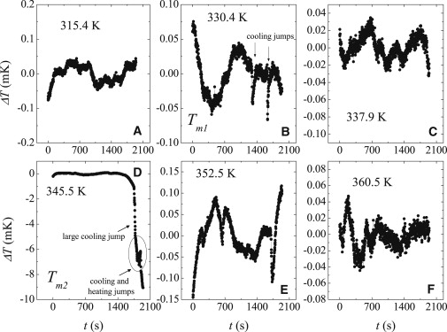
Figs. 4 and 5 show the timeseries of temperature fluctuations at different temperatures for the 100-bp heteropolymer and the 40-kbps DNA, respectively. It can be seen from the plots that the fluctuations evolve as a function of temperature and the observed fluctuation at T ∼ T_m1 is different from that seen at T ∼ T_m2.

Figure 4.

Time series of temperature fluctuations for the 100-bp heteropolymer at different temperatures.

Figure 5.

Time series of temperature fluctuation for the 40-kbps T7 DNA at different temperatures.

Below T_m1, the fluctuations are small and there are similar number of heating and cooling jumps. At T ∼ T_m1 the timeseries is characterized by what can be called “jumps-and-pauses” behavior, which consists of cooling jumps followed by pause periods where the fluctuation is small. To guide the reader, the cooling jumps are marked by arrows in Figs. 4 D and 5 B. These cooling jumps arise due to opening up of basepairs or creation of denaturated bubbles, which causes energy absorption from the substrate. This “jumps-and-pauses” behavior persists until T_m2. As T → T_m2, the timeseries changes nature and the fluctuations become larger. The fluctuations at T_m2 start with several cooling and heating jumps. This is followed by a rather large cooling jump, which is followed by a recovery (the returning of the SSS to the reservoir temperature), as can be seen from the T ≈ 361 K plots for the 100-bp heteropolymer. After this large jump, large fluctuations are completely absent. This means that almost the entire DNA is denatured due to opening of the GC bonds at the major transition which can be thought of as a cooperative or coordinated transition. To our knowledge, such features of the denaturation transition have not been observed before and this gives a new dimension to the denaturation process.

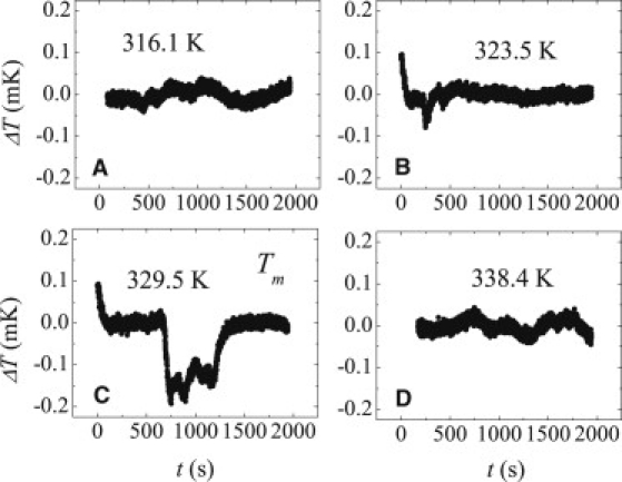
Fig. 6 shows the timeseries for the 100 bp ..ATAT.. homopolymer at temperatures close to its T_m (∼331 K). At, or very close to the melting temperature, the homopolymer shows very small, mostly cooling jumps (few hundred μK). Other than this, there are no large fluctuations. There may be two reasons for the absence of large fluctuations in the homopolymer:

• 1.The fluctuation may actually be small due to the absence of heterogeneity and/or
• 2.They occur at a timescale that is much faster than the detection bandwidth of the calorimeter.

This can be seen from Eq. 4, which in the limit τ_P << τ_th gives ΔT_jump = τ_PP_P/C_sub. As a result, for very small τ_P and/or very small P_P, ΔT_jump can be very small. Unless these experiments are performed using a calorimeter that has a much smaller τ_th that is comparable to τ_P, this particular issue cannot be resolved.

Figure 6.

Time series of temperature fluctuation for the 100-bp homopolymer (..ATAT..) at different temperatures.

A very important issue that arises in an experiment of this type, is the reproducibility of the data. To compare results of fluctuations from different samples, it is important to know how the fluctuations scale with the mass of the sample. For checking the scaling with mass, we carried out the experiments with different amounts of sample. Fig. 7 shows the 〈(ΔT)²〉/T² for 17 μg of 100 bp heteropolymeric DNA. In the same graph, we show 4 × 〈(ΔT)²〉/T² for 8.5 μg of the sample. We see that the two data sets match very well, proving reproducibility of the data and scaling of the fluctuations with mass. (Note: Because ΔT ∝ ΔH and ΔH ∝ m, m = sample mass, the quantity 〈(ΔT)²〉/T² is thus expected to be ∝ m² .)

Figure 7.

Scaling of fluctuations with mass. 〈(ΔT)²〉/T² for 17-μg 100-bp heteropolymeric dsDNA (shown by open squares) and that for 8.5 μg of the DNA multiplied by four (shown by solid circles).

Discussion

Analysis of the time series

We start the discussion by a quantitative analysis of the time series. The enthalpy exchanged between the DNA and the calorimeter can be obtained by analyzing the time series data using Eq. 4. Briefly, for each temperature jump the jump magnitude ΔT_jump and jump width τ_P are obtained. From the jump magnitude the power of the pulse P_P is calculated. The enthalpy exchanged E_P = P_Pτ_P is obtained for each pulse and the enthalpies at a particular temperature are added to get the total enthalpy ΔH = ΣE_P absorbed/released at that temperature.

We calculate that, for the 100-bp heteropolymer, the total enthalpy exchanged in the jumps at T_m1 is ≈ 6.1 J/g. In the heteropolymer, the fraction of AT bases is 48%, giving the bond energy of AT as 12.6 J/g. The total enthalpy exchanged at T_m2 is ≈ 8.8 J/g. The fraction of GC bonds in the heteropolymer is 52%, giving the bond energy of GC as 17 J/g. The energy of the AT/GC bond observed/calculated previously depends on its nearest neighbors (12–14). The reported values vary between 6 J/g and 13 J/g for an AT bond and between 9 J/g and 20 J/g for a GC bond (12–16). (Note that although several works have reported several values of energy (12-16), it is common consensus that an AT bond or an AT-rich region requires lower energy to denature than a GC bond or a GC-rich region.) Our values lie within the reported range of values for AT/GC bonds. Therefore the assignment of T_m1 as the temperature where the AT bonds in the heteropolymer break and of T_m2 as the temperature where the GC bonds break is supported by the energetics of the process. This analysis clearly shows that the first peak corresponds to the denaturation of AT-rich regions forming bubbles. The second peak corresponds to denaturation of GC-rich regions ending with the entire DNA separating out. The first peak T_m1 occurs at a temperature slightly (∼3 K) higher than T_m–AT. The denaturation bubbles are in AT regions but, being a heteropolymer, these regions consist of a small fraction of GC basepairs which raises T_m1 in comparison to T_m–AT. Similarly, T_m2 is lower than T_m–GC. This comes about because at temperatures between T_m1 and T_m2, GC rich regions bind the AT rich loops. Base-stacking interactions lower the energy required for the denaturation of the GC rich regions. This causes them to denature at temperatures lower than a ..GCGC.. homopolymer denaturation temperature.

From the analysis of the temperature jump data we can make an estimate of the distribution of enthalpy exchanged in the jumps. We consider the region close to T_m2. Fig. 8 shows a distribution of E_P per gram of GC bond at 361 K for the 100-bp heteropolymer. The energy scales shown in the figure are in J/g of sample. A quantity of 1 J/g corresponds to 43.8 k_BT per 100-bp dsDNA. The distribution of E_P is rather broad and has both energy-absorbing jumps (negative) and energy-releasing jumps (positive). However, the energy-absorbing jumps occur with a higher probability, showing that the process (melting) is proceeding in a direction where there are more basepairs opening up than closing. Fig. 9 shows the distribution of the pulse-width τ_P for both energy-releasing and energy-absorbing jumps at 361 K. There is a clear asymmetry in the value of τ_P. For the cooling jumps, τ_P is 4.25 ± 0.5 s and for heating jumps, τ_P is smaller and is equal to 1.75 ± 0.5 s.

Figure 8.

Distribution of E_P per gram of GC bond at 361 K (T_m2) for the 100-bp heteropolymer.

Figure 9.

Distribution of τ_P for energy-absorbed and energy-released jumps at 361 K (T_m2) for the 100-bp heteropolymer.

Probability distribution function and nature of the fluctuation

The nature of the observed fluctuation can be studied using the probability distribution function (PDF). According to the central-limit theorem (17), if the fluctuators are uncorrelated, the PDF of the fluctuation is Gaussian. Deviation from Gaussianity arises when the fluctuators are correlated. Thus, the PDF is one way to check whether the system has any cooperativity involved. We find that the observed fluctuation in the heteropolymers is Gaussian above T_m2, while it assumes a strongly non-Gaussian nature close to the melting temperature range. The non-Gaussianity is present even in the homopolymer.

The PDF essentially is a distribution of the probability of occurrence of a temperature jump of certain magnitude. The bin size used in the calculation of PDF is 3 μK. (Note that this particular bin size is selected because the bin size used has to be larger than the thermal background contribution and the resolution of the system. In this case, the system resolution is ≈2 μK.) Shown in Fig. 10 are the PDFs for the 100-bp heteropolymer and the 100-bp ..ATAT.. homopolymer. For a Gaussian distribution, P(ΔT) ∼ exp(– (ΔT)²/(2σ²)), where σ is the variance. Therefore, the plots of lnP(ΔT) versus (ΔT)² should be straight lines. It is immediately obvious that heteropolymeric DNA shows large deviation from Gaussianity close to the melting temperature. We find that the PDF for the heteropolymer can be expressed as a summation of a Gaussian and a power-law behavior, particularly when close to the melting temperature. For the homopolymer the fluctuation is not strictly a Gaussian, but can be expressed as a sum of two Gaussians.

Figure 10.

PDF at a few representative temperatures (which includes their T_m) for (A) 100-bp heteropolymer and (B) 100-bp ..ATAT.. homopolymer.

We explain the appearance of non-Gaussianity using the following scenario: In the DNA, every base can either be bound to its pair or be unbound. Thus, the bond between each basepair can be in either open or closed state. This state of the bond is the fluctuating quantity and is the origin of fluctuation. If the bonds are independent of each other, the temperature fluctuations will be Gaussian. In the case of DNA, the opening up of one basepair can cause adjacent basepairs to open up due to base-stacking interactions. Here, in addition to the energy cost for a basepair opening and the compensatory entropy gained, there is an additional energy cost for disruption of the base stacking (an energy is needed to keep one basepair open and the next one closed). Thus, the fluctuators are not independent. This correlation between the fluctuators is present even for homopolymers and can cause the PDF to become non-Gaussian.

For a heteropolymeric DNA, some regions have a higher probability of opening up than others. This is because the energy required for breaking an AT bond is lower than the energy required for breaking a GC bond. This will cause AT-rich regions to open up at lower temperatures, while GC-rich regions will remain bound until higher temperatures. Here again, the fluctuations are not independent. It can be seen from Fig. 10 that the 100-bp heteropolymer shows a very severe non-Gaussian behavior, particularly at ∼T_m2. It can also be noted that even for T_m2 > T > T_m1, the PDF is non-Gaussian. In this region there are basepairs which are in dynamic equilibrium between open and closed states. This would cause adjacent basepairs also to open and close. This leads to correlations which cause the PDF to become non-Gaussian. The PDF becomes Gaussian above T_m2. This indicates that well above T_m2, the two strands of the DNA are completely separated-out and there is not much interaction between the strands except for, probably, some nonspecific bonding.

Thermal fluctuation in dsDNA—a simple proposed model

The models of DNA denaturation (1,2,18,19) are based on the idea that the bonds have two states accessible to them—open or closed. For the DNA, due to base-stacking energy, it is energetically favorable to have an open basepair next to another open basepair. Thus, competition between the base-stacking energy; the energy required to break a basepair bond; and the entropy of an unbound region decide whether a basepair will be open or closed. These energies and entropy depend on temperature, and thus, the probability of a bond being open or closed will depend on temperature. In our experiments we have studied the DNA denaturation starting from a low temperature (300 K) where we expect the DNA to be fully closed. Increase in temperature will cause an increase in the fraction of open basepairs and open regions. However, DNA being a dynamic system, open (or closed) basepairs will not always remain open (closed), and can close (open) when, due to random walk executed by the loop, the bases come together. This opening and closing of the basepairs has energetics associated with it and causes the temperature fluctuations that we measure. The observed fluctuations using TFS will be large when there is a sudden or cooperative change in state for a large number of basepairs.

In a homopolymer, the bases are identical. Thus, the probability for opening is the same for every bond. It can be expected that the bubbles have an equal probability of existing anywhere in the DNA and there can be coexistence between different similar energy configurations. However, as shown recently, nonlinear localization lifts this degeneracy and causes opening of some specific bonds at low temperature (20). The size of these open regions increases with temperature, leading to bubble formation. Again, these bubbles are more probable in some regions of the DNA, which are called hot patches. Increase in temperature causes more basepairs to open up, leading to a smooth melting transition. As far as the fluctuations are concerned, we observe them to be small, as compared with heteropolymeric dsDNA. This is understandable, as there is no sudden opening up of large regions of dsDNA which could cause large fluctuations.

In a dsDNA heteropolymer, an additional factor comes into play—the bonds are now not identical. The energy of an AT bond is lower than that of a GC bond. In addition, the base-stacking energies are now different. This causes AT-rich and GC-rich regions to behave differently. The sequence of denaturation of a heteropolymeric DNA which can provide a qualitative scenario for the observed data is schematically portrayed in Fig. 11. At temperatures T ≈ T_m1, the AT-rich regions of the heteropolymer denature, giving rise to bubbles. The size of the bubbles depend on the size of the AT-rich regions. The formation of these bubbles causes a lowering of the calorimeter temperature, leading to cooling jumps. The formation of these bubbles thus causes an increase in the thermal fluctuation over the background value. Given the statistical nature of the bubble formation, one obtains a random time series. These bubbles are not allowed to propagate along the DNA by the GC-rich regions. It is this that localizes the bubbles in certain sections of DNA, leading to the jumps-and-pauses behavior seen at ∼T_m1. When the temperature reaches T_m2, some GC bonds, which were acting as barriers to the denaturation, start to open. The opening up of sufficient number of the GC bonds causes the energy barriers for denaturation to collapse. This causes the entire DNA to suddenly open up, leading to a major, cooperative transition which we see in the time series at T = T_m2 (see Figs. 4 and 5). This transition has a large energy associated with it and shows up as a large cooling jump. Superposed on the jumps are the smaller heating and cooling jumps caused by the opening and closing of basepairs. The major transition has associated with it large changes in energy, leading to large changes in the substrate temperature, causing the fluctuation to peak at this temperature. After the transition is complete, the temperature of the substrate recovers back to the reservoir temperature.

Figure 11.

Schematic of the denaturation process for a heteropolymeric DNA. In the case of a heteropolymer, each bond is different from the others and there is interaction between the bonds. (The AT bond is represented by a blue line and the GC bond is represented by a red line.)

To summarize, we have developed the technique of thermal fluctuation spectroscopy to study the denaturation dynamics of a system. We used this technique to study the thermal denaturation of DNA and showed that the denaturation of heteropolymeric dsDNA is accompanied by large, non-Gaussian thermal fluctuations. The thermal fluctuations show a two-peak structure. We calculated the enthalpy exchanges causing the fluctuations and showed from it that the first peak arises due to denaturation of AT-rich regions and the second due to denaturation of GC-rich regions. The large fluctuation is almost absent in homopolymeric DNA. We suggest that bubble formation and cooperative opening and closing dynamics of basepairs causes the additional fluctuation at the first peak and a large cooperative transition from a partially molten DNA to a completely denatured state causes the additional fluctuation at the second peak. Simulation of the denaturation process to explain the observed data will be a welcome step forward.

References

- 1.Poland D., Scheraga H.A. Phase transitions in one dimension and the helix-coil transition in polyamino acids. J. Chem. Phys. 1966;45:1456–1463. doi: 10.1063/1.1727785. [DOI] [PubMed] [Google Scholar]
- 2.Poland D., Scheraga H.A. Occurrence of a phase transition in nucleic acid models. J. Chem. Phys. 1966;45:1464–1469. doi: 10.1063/1.1727786. [DOI] [PubMed] [Google Scholar]
- 3.Rouzina I., Bloomfield V.A. Heat capacity effects on the melting of DNA. 1. General aspects. Biophys. J. 1999;77:3242–3251. doi: 10.1016/S0006-3495(99)77155-9. [DOI] [PMC free article] [PubMed] [Google Scholar]
- 4.Barbi M., Lepri S., Theodorakopoulos N. Thermal denaturation of a helicoidal DNA model. Phys. Rev. E Stat. Nonlin. Soft Matter Phys. 2003;68:061909. doi: 10.1103/PhysRevE.68.061909. [DOI] [PubMed] [Google Scholar]
- 5.Essevaz-Roulet B., Bockelmann U., Heslot F. Mechanical separation of the complementary strands of DNA. Proc. Natl. Acad. Sci. USA. 1997;94:11935–11940. doi: 10.1073/pnas.94.22.11935. [DOI] [PMC free article] [PubMed] [Google Scholar]
- 6.Danilowicz C., Coljee V.W., Prentiss M. DNA unzipped under a constant force exhibits multiple metastable intermediates. Proc. Natl. Acad. Sci. USA. 2003;100:1694–1699. doi: 10.1073/pnas.262789199. [DOI] [PMC free article] [PubMed] [Google Scholar]
- 7.Cocco S., Monasson R., Marko J.F. Force and kinetic barriers to unzipping of the DNA double helix. Proc. Natl. Acad. Sci. USA. 2001;98:8608–8613. doi: 10.1073/pnas.151257598. [DOI] [PMC free article] [PubMed] [Google Scholar]
- 8.Lubensky D.K., Nelson D.R. Pulling pinned polymers and unzipping DNA. Phys. Rev. Lett. 2000;85:1572–1575. doi: 10.1103/PhysRevLett.85.1572. [DOI] [PubMed] [Google Scholar]
- 9.Nagapriya K.S., Raychaudhuri A.K., Chatterji D. Direct observation of large temperature fluctuations during DNA thermal denaturation. Phys. Rev. Lett. 2006;96:038102. doi: 10.1103/PhysRevLett.96.038102. [DOI] [PubMed] [Google Scholar]
- 10.Nierman W.C., Chamberlin M.J. Studies of RNA chain initiation by Escherichia coli RNA polymerase bound to T7 DNA. Direct analysis of the kinetics and extent of RNA chain initiation at T7 promoter A1. J. Biol. Chem. 1979;254:7921–7926. [PubMed] [Google Scholar]
- 11.Ghosh, A., S. Kar, …, A. K. Raychaudhuri. 2004. A set-up for measurement of low frequency conductance fluctuation (noise) using digital signal processing techniques. arXiv:cond-mat/0402130v1 [cond-mat.other].
- 12.Breslauer K.J., Frank R., Marky L.A. Predicting DNA duplex stability from the base sequence. Proc. Natl. Acad. Sci. USA. 1986;83:3746–3750. doi: 10.1073/pnas.83.11.3746. [DOI] [PMC free article] [PubMed] [Google Scholar]
- 13.SantaLucia J. A unified view of polymer, dumbbell, and oligonucleotide DNA nearest-neighbor thermodynamics. Proc. Natl. Acad. Sci. USA. 1998;95:1460–1465. doi: 10.1073/pnas.95.4.1460. [DOI] [PMC free article] [PubMed] [Google Scholar]
- 14.Delcourt S.G., Blake R.D. Stacking energies in DNA. J. Biol. Chem. 1991;266:15160–15169. [PubMed] [Google Scholar]
- 15.Doktycz M.J., Goldstein R.F., Benight A.S. Studies of DNA dumbbells. I. Melting curves of 17 DNA dumbbells with different duplex stem sequences linked by T4 endloops: evaluation of the nearest-neighbor stacking interactions in DNA. Biopolymers. 1992;32:849–864. doi: 10.1002/bip.360320712. [DOI] [PubMed] [Google Scholar]
- 16.Sugimoto N., Nakano S., Honda K. Improved thermodynamic parameters and helix initiation factor to predict stability of DNA duplexes. Nucleic Acids Res. 1996;24:4501–4505. doi: 10.1093/nar/24.22.4501. [DOI] [PMC free article] [PubMed] [Google Scholar]
- 17.Reif F. 1st Ed. McGraw-Hill; New York: 1965. Fundamentals of Statistical and Thermal Physics. [Google Scholar]
- 18.Poland D., Scheraga H.A. 1st Ed. Academic Press; New York: 1970. Theory of Helix-Coil Transitions in Biopolymers. [Google Scholar]
- 19.Nelson D.R. Statistical physics of unzipping DNA. In: Skjeltorp A.T., Belushkin A.V., editors. Forces, Growth and Form in Soft Condensed Matter: At the Interface between Physics and Biology. Springer; Dordrecht, The Netherlands: 2005. [Google Scholar]
- 20.Peyrard M., Farago J. Nonlinear localization in thermalized lattices: application to DNA. Physica A. 2000;288:199–217. [Google Scholar]