How Long Does It Take to Establish a Morphogen Gradient?

Abstract

A morphogen gradient is defined as a concentration field of a molecule that acts as a dose-dependent regulator of cell differentiation. One of the key questions in studies of morphogen gradients is whether they reach steady states on timescales relevant for developmental patterning. We propose a systematic approach for addressing this question and illustrate it by analyzing several models that account for diffusion and degradation of locally produced chemical signals.

One of the key questions in studies of morphogen gradients is whether they reach steady states on timescales relevant for developmental patterning (1–3). Although Crick posed this question 40 years ago (4), a general formalism for addressing this question is still lacking. Here we suggest a method for tackling this problem in an important class of biophysical models that account for diffusion and degradation of locally produced chemical signals.

We begin with a simple model that is commonly used as a first step in the analysis of more complex mechanisms of morphogen gradient formation and interpretation (5). Let C(x,t) be the concentration at a distance x > 0 from the boundary, where a morphogen is produced at a constant rate Q. Signal production begins at t = 0, when C(x,t) = 0 throughout the system. The concentration satisfies

$$\begin{array}{l}\frac{\partial C}{\partial t}=D\frac{{\partial }^{2}C}{\partial x^2}-kC,C\left(x,t=0\right)=0,\\ -D{\frac{\partial C}{\partial x}|}_{x=0}=Q,C(x=\infty )=0.\end{array}$$

Here D is the diffusivity and k is degradation rate constant.

First, we consider the total amount of morphogen accumulated in the system by time t:

$$N\left(t\right)=\underset{0}{\overset{\infty }{\int }}C\left(x,t\right)dx\text{.}$$

One can show that N(t) starts from zero and exponentially approaches its steady-state value N_s = Q/k,

$$N\left(t\right)=N_s\left(1-\exp \left(-kt\right)\right)\text{.}$$

To quantify the approach to the steady state, we introduce the relaxation function, denoted by R_N(t). This function is defined as the ratio of the difference between the current and steady-state values of N(t) to this difference at t = 0,

$$R_N\left(t\right)=\frac{N\left(t\right)-N_s}{N\left(0\right)-N_s}=\exp \left(-kt\right)=\exp \left(-t/{\tau }_N\right)\text{,}$$

where the decay time, τ_N = 1/k, is independent of the diffusivity and the signal production rate. Thus, for the total amount of morphogen in the system, the relaxation to the steady state is exponential.

Similarly, we introduce the local relaxation function, R(x,t), to analyze the approach of C(x,t) to C_s(x), its steady-state value at a given x:

$$R\left(x,t\right)=\frac{C\left(x,t\right)-C_s\left(x\right)}{C\left(x,0\right)-C_s\left(x\right)}=1-\frac{C\left(x,t\right)}{C_s\left(x\right)}\text{.}$$

This function monotonically decays with time from unity at t = 0 to zero as time tends to infinity. The initial and final values of R(x,t) are independent of x, but the relaxation kinetics clearly depends on position.

To characterize this kinetics by a single timescale we use the fact that the fraction of the steady-state concentration at point x accumulated between t and t+dt is given by

$$\left[-\partial R\left(x,t\right)/\partial t\right]dt\text{.}$$

Therefore, the negative derivative of the relaxation function is the probability density for the time of the local accumulation process,

$$\phi \left(t|x\right)=-\partial R\left(x,t\right)/\partial t\text{.}$$

We use this probability density to find the mean time τ(x),

$$\tau \left(x\right)=\underset{0}{\overset{\infty }{\int }}t\phi \left(t|x\right)dt=\underset{0}{\overset{\infty }{\int }}R\left(x,t\right)dt\text{,}$$

which is the local relaxation time to steady state at point x.

To show how this formalism works, we first use the known solution for C(x,t) (3):

$$C\left(x,t\right)=C_s\left(x\right)\left[1-\frac{1}{2}erfc\left(\frac{\sqrt{Dt}}{\lambda }-\frac{x}{2\sqrt{Dt}}\right)-\frac{1}{2}{e}^{\frac{2x}{\lambda }}erfc\left(\frac{\sqrt{Dt}}{\lambda }+\frac{x}{2\sqrt{Dt}}\right)\right]\text{,}$$

where erfc(z) is the complementary error function, $\lambda =\sqrt{D/k}$, and C_s(x) is the steady state (Fig. 1 A):

$$C_s\left(x\right)=\frac{Q}{\sqrt{Dk}}\exp \left(-\frac{x}{\lambda }\right)\text{.}$$

From this, we find the local relaxation function,

$$R\left(x,t\right)=\frac{1}{2}erfc\left(\frac{\sqrt{Dt}}{\lambda }-\frac{x}{2\sqrt{Dt}}\right)+\frac{1}{2}{e}^{2x/\lambda }erfc\left(\frac{\sqrt{Dt}}{\lambda }+\frac{x}{2\sqrt{Dt}}\right)$$

and then integrate over time to obtain the local relaxation time,

$$\tau \left(x\right)=\frac{1}{2k}\left(1+\frac{x}{\lambda }\right)\text{.}$$

The linear dependence of this time on x is surprising. Indeed, one can think about two timescales associated with the relaxation to steady state at point x, namely, the characteristic times of reaction and diffusion, defined respectively as τ_r = 1/k = τ_N and τ_d(x) = x²/2D. One might expect that the relaxation is controlled by the larger of the two times. The formula for τ(x) shows that this argument is applicable only when x << λ and fails when x >> λ. Indeed, when x << λ, the relaxation time is determined purely by degradation and τ(x) ≈ τ_r/2. However, when x >> λ, both degradation and diffusion are equally important, and the relaxation time is given by

$$\tau \left(x\right)\approx {\left({\tau }_r{\tau }_d\left(x\right)/2\right)}^{1/2}\text{.}$$

For practical purposes, however, one is interested in the intermediate regime, because gradients typically control gene expression on length scales comparable to λ.

Figure 1.

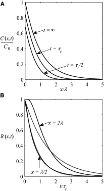
(A) Concentration profile at three different times. The concentration has been scaled by the maximal concentration at x = 0, $C_0=Q/\sqrt{Dk}$. (B) The exact relaxation function, R(x,t), is plotted as a function of dimensionless time for x = λ/2 and x =2λ. (Dashed lines) Exponential approximation of the relaxation function, R_exp(x,t).

We can use the derived expression for τ(x) to discuss the steady-state approximation in the analysis of the first identified morphogen gradient. This gradient is formed by Bicoid (Bcd), a transcription factor which patterns the anteroposterior axis of the Drosophila embryo by specifying the expression boundaries of multiple genes (6). In the textbook model of this gradient, Bcd forms an exponentially distributed concentration profile, which is believed to result from the combined effects of localized production, diffusion, and uniform degradation. The observed gradient is indeed well approximated by an exponential function with λ ∼75 μm. However, whether this function can be interpreted as the steady state of an underlying reaction-diffusion model is currently a matter of debate, mainly due to the uncertainty in the values of Bcd diffusivity and degradation rate constant (7).

The most distant gene expression boundary controlled by Bcd is located 375 μm from the source of Bcd production, hence x/λ ≈ 5. Because the Bcd gradient is formed in 90 min, the expression for τ(x) provides an upper limit on the Bcd lifetime: τ_r > 30 min. Furthermore, based on the expression for λ, we obtain the following lower limit for Bcd diffusivity: D > 3 μm²/s. Similar calculations can be carried out for more complex models to evaluate the candidate or the experimentally measured values of Bcd diffusivity and lifetime.

Above we discussed the model for which a closed form solution for the dynamics of the morphogen field is known. However, our approach is equally applicable to linear models where a closed form solution is unavailable. These models, which play an important role in the current literature on morphogen gradients, may account for the effects of a spatially distributed source of morphogen production, finite length of the patterned field, reversible binding of morphogen molecules by localized traps, and cascades of reaction-diffusion modules (5).

Analysis of these models can be based on the Laplace transform of the relaxation function:

$$\widehat{R}\left(x,s\right)=\underset{0}{\overset{\infty }{\int }}R\left(x,t\right)e^{-st}dt\text{.}$$

From this expression, it follows that

$$\tau \left(x\right)=\widehat{R}\left(x,s=0\right)\text{.}$$

An important advantage of the Laplace transform-based approach is that it does not require the explicit solution for C(x,t).

As an example, we use a model where the source of morphogen production is not sharply localized, as above, but distributed in a gradient with a characteristic length scale λ_s:

$$Q\left(x\right)=\left(Q/{\lambda }_s\right)\exp \left(-x/{\lambda }_s\right)\text{.}$$

Such a model has been recently proposed for the Bcd gradient, based on the visualization of the spatial distribution of bcd mRNA (8). The discussion of this model in the context of other mechanisms of the Bcd gradient formation can be found in recent reviews (6,7). The steady state in this model is given by the expression

$$C_s\left(x|{\lambda }_s\right)=\frac{Q{\lambda }^2}{D\left({\lambda }^2-{\lambda }_s^2\right)}\left(\lambda e^{-x/\lambda }-{\lambda }_s{e}^{-x/{\lambda }_s}\right)$$

and the relaxation time is given by

$$\tau \left(x|{\lambda }_s\right)=\frac{1}{2k}\left[\left(1+\frac{x}{\lambda }\right)\frac{\lambda e^{-x/\lambda }}{\lambda e^{-x/\lambda }-{\lambda }_s{e}^{-x/{\lambda }_s}}+\frac{2{\lambda }_s^2}{{\lambda }_s^2-{\lambda }^2}\right]\text{.}$$

When λ_s << λ, the formula reduces to the local relaxation time derived above. On the other hand, when λ << λ_s, the relaxation time is independent of x and equal to the characteristic time of reaction, τ(x) = τ_r = 1/k. Note that if the Bcd gradient is indeed established in the regime where λ << λ_s, then Bcd diffusivity can be much smaller than the values allowed by the localized source model.

As another example, we consider the model where the length of the patterned interval is finite. In addition to morphogenetic patterning, this model is relevant for the analysis of intracellular chemical gradients, e.g., when a protein is phosphorylated at the cell membrane, diffuses inside the cell, and is degraded by a uniformly distributed phosphatase (9). In this case, the steady-state concentration is given by

$$C_s\left(x|L\right)=\frac{Q\cosh \left(\left(\left(L-x\right)\right)/\lambda \right)}{\sqrt{Dk}\sinh \left(L/\lambda \right)}\text{,}$$

where L is the size of the system. Using the Laplace transform, we derived the local relaxation time:

$$\tau \left(x|L\right)=\frac{1}{2k}\left[1+\frac{L}{\lambda }\coth \left(\frac{L}{\lambda }\right)-\frac{L-x}{\lambda }\tanh \left(\frac{L-x}{\lambda }\right)\right]\text{.}$$

When L → ∞, τ(x|L) reduces to the local relaxation time for the semiinfinite interval. In the opposite extreme, when λ >> L, the relaxation time is independent of x and is equal to the degradation time 1/k.

Based on the local relaxation time, one can estimate the time needed to reach a specific concentration threshold value θ, at a given point x (2,3). This time, denoted by t_θ(x), satisfies the C(x,t_θ(x)) = θ, which is equivalent to

$$1-R\left(x,t_{\theta }\left(x\right)\right)=\theta /C_s\left(x\right)\text{.}$$

An approximate solution can be obtained by constructing an exponential approximation of the exact relaxation function (Fig. 1 B):

$$R\left(x,t\right)\approx R_{\exp }\left(x,t\right)=\exp \left(-t/\tau \left(x\right)\right)\text{.}$$

Then, the approximate solution for t_θ(x) is given by

$$t_{\theta }\left(x\right)\approx \tau \left(x\right)\ln \left(\frac{C_s\left(x\right)}{C_s\left(x\right)-\theta }\right)\text{.}$$

Importantly, this expression does not depend on the time-dependent solution and can be used to analyze problems where a closed form solution for C(x,t) is unavailable.

In conclusion, we proposed formalism for analyzing how the local concentration of a morphogen approaches its steady state in models that account for diffusion and uniform degradation of a locally produced signal. For systems where there are direct measurements of the diffusivity and degradation rate constant (10,11), our results can be used to directly calculate the timescale for reaching the steady state. For systems where D and k are unavailable, our results can be used to constrain their values based on the experimentally observed gradients and estimates of the time during which the gradient is acting.