

Abstract
Obtaining quantitative kinetic parameters from fluorescence recovery after photobleaching (FRAP) experiments generally requires a theoretical analysis of protein mobility and appropriate solutions for FRAP recovery derived for a given geometry. Here we provide a treatment of FRAP recovery for a molecule undergoing a combined process of reversible membrane association and lateral diffusion on the plasma membrane for two commonly used bleach geometries: stripes, and boxes. Such analysis is complicated by the fact that diffusion of a molecule during photobleaching can lead to broadening of the bleach area, resulting in significant deviations of the actual bleach shape from the desired bleach geometry, which creates difficulty in accurately measuring kinetic parameters. Here we overcome the problem of deviations between actual and idealized bleach geometries by parameterizing, more accurately, the initial postbleach state. This allows for reconstruction of an accurate and analytically tractable approximation of the actual fluorescence distribution. Through simulated FRAP experiments, we demonstrate that this method can be used to accurately measure a broad range of combinations of diffusion constants and exchange rates. Use of this method to analyze the plextrin homology domain of PLC-δ1 in Caenorhabditis elegans results in quantitative agreement with prior analysis of this domain in other cells using other methods. Because of the flexibility, relative ease of implementation, and its use of standard, easily obtainable bleach geometries, this method should be broadly applicable to investigation of protein dynamics at the plasma membrane.
Introduction
To understand the dynamic processes that underlie the structure, organization, and diverse behaviors of cells, we require kinetic information about the behavior of proteins involved. Ideally, this information will be obtained within the milieu where these processes occur—inside living cells. Fluorescence recovery after photobleaching (FRAP) is an attractive method for such purposes due to its relative ease of implementation using the current generation of confocal microscopes.
In a typical FRAP experiment, a fluorescent molecule is irreversibly bleached within a small region of interest (ROI) using high intensity laser light. Fluorescence then recovers as the population of bleached molecules is replaced by unbleached molecules from outside the ROI. Because the kinetics of this recovery reflect the underlying dynamics of the molecule of interest, FRAP experiments can tell us a great deal about the mobility of molecules within cells. Much has been gained from simple inspection of FRAP recovery curves, including determining the rates of local protein turnover, identifying immobile fractions, and demonstrating exchange between cellular compartments or lack thereof (1). At the same time, because a molecule's dynamics within the cell will be determined by a combination of molecular mobilities, including both diffusion and bulk transport, and its binding interactions with components within the cell, FRAP experiments have the potential to allow measurement of key kinetic parameters, including the relevant rate constants.
Here we examine the case of FRAP analysis of a membrane-associated molecule. We consider a common case in which the mobility of this molecule within the cell is determined by three behaviors: reversible plasma membrane association, lateral diffusion in the membrane-associated state, and free, rapid diffusion in the cytoplasm. Analysis of FRAP recovery when binding reactions dominate is relatively straightforward. In such cases where binding can be uncoupled from the effects of diffusion, recovery should follow an exponential (2). However, if diffusion contributes significantly to protein mobility at the relevant length and timescales, FRAP analysis is significantly more complicated. Notably, because recovery by diffusion is not spatially uniform across the bleached region, diffusion will change the shape of the bleached region over time, a phenomenon which itself provides evidence for lateral diffusion within cells (3–6).
Mathematical solutions for extracting diffusion constants have been derived in several cases (5,7,8), including solutions for mixed recovery due to lateral diffusion and binding (9–11). However, many FRAP regimes for analyzing molecular diffusion make unrealistic assumptions. For example, most assume instantaneous bleaching and neglect the effect of diffusion of molecules during the bleach period. For fast diffusing species, diffusion during bleaching leads to significant deviations of the actual bleach spot from the theoretical bleach spot. This phenomenon leads to a so-called halo effect in which the edges of the bleached region are not sharp (e.g., Fig. S1 B in the Supporting Material), but, instead, fluorescence intensity undergoes a smooth transition between the bleached and unbleached regions. If not properly accounted for, such factors can easily lead to significant errors in FRAP analysis (12–15). Recently, efforts have been made to avoid these effects and to make use of the spatiotemporal aspects of the recovery to extract additional mobility properties (14,15).
To circumvent the difficulties in analysis introduced by diffusion, one can attempt to describe, more accurately, the initial fluorophore distribution (i.e., the initial state) and minimize the deviation between the actual and theoretical bleached area. Several solutions have been proposed. One is to take the initial fluorescence distribution and numerically calculate the expected evolution using a kinetic model and identify the parameters that yield the best fit to experimental data (16,17). In practice, it is often favorable to have an analytical description of the expected recovery for a set of simple bleach geometries that can be used for fitting. To date, analytic solutions exist for only a subset of shapes (e.g.. box, disk, stripe), most of which are defined by sharp boundaries and thus are not capable of accurately capturing an actual bleach profile that exhibits spreading due to lateral diffusion. One exception: Gaussian bleach profiles, which have the advantage that they remain Gaussian through time (5). Here we present a solution for two common non-Gaussian bleach geometries—a simple box or square, and its one-dimensional equivalent, a stripe—both of which are easily implemented and offer advantages over Gaussian spots in certain applications.
The method we describe relies on the fact that a distribution of particles initially characterized by a step-function (e.g., a sharp boundary) will progressively evolve into a smooth distribution if subjected to diffusion. Specifically, the distribution of particles in such a system can be described analytically in terms of an error function at all times (see Eqs. 4, 6, and 7). Therefore, we can use error functions to describe the boundaries of a given bleach region to capture both the extent of the bleach region (e.g., box width) and the gradient of fluorescence at the edges. The evolution of the fluorescence distribution can then be determined by calculation of the time evolution of these error functions.
We provide a closed-form solution that describes the evolution of fluorescence intensity integrated over the bleach area after photobleaching for recovery due to membrane-cytoplasm exchange and lateral diffusion. This solution should exactly describe an experiment in which a region with sharp edges is bleached instantaneously, but the first postbleach frame is captured at some inevitable time delay. In reality, the bleach period will be of finite duration resulting in diffusive spreading of the bleach region during bleaching. Optical limitations also ensure that the edges of a bleach region are not infinitely sharp. Such effects give rise to distributions that do not take the exact form of error functions. However, the resulting smoothening of the boundary is still well described by error functions. As long as the initial bleach distribution is reasonably well characterized by error functions, the solution we provide allows for accurate measurements of diffusion and exchange kinetics. Importantly, one is left free to choose an initial postbleach frame best suited to the particular experimental details. As such, we believe this method should provide a useful tool for analyzing the behavior of membrane-associated proteins in a variety of systems.
Theory
Reversible membrane binding and lateral diffusion
Let us consider a spatially extended system consisting of a cytoplasmic volume surrounded by a membrane, populated by a molecule of interest, the total quantity of which is conserved. This molecule exists in one of two states, membrane-associated or cytoplasmic. Its local density on the membrane is given by a and in the cytoplasm by b. We will consider the case where the mobility of this molecule can be described by three processes: Lateral diffusion on the membrane is described by a diffusivity D, diffusion in bulk cytoplasm is described by Dc, and transitions between the two states are governed by mass action kinetics with binding coefficients kon and koff. These transitions take the form of a boundary flux for diffusion in bulk. This system can be described as
| (1) |
| (2) |
where ∇2 denotes the two-dimensional Laplace operator, the diffusive flux is given by
within the cytoplasm, and b|surf denotes the volume concentration of proteins in the infinitesimal bulk volume element that interacts with the surface at a. Conservation of protein number is ensured through the boundary conditions for Eq. 2 at the membrane-cytoplasm interface, which take the form of an additional flux
at the surface, where is the unit vector normal to the surface, pointing outwards.
Several simplifying assumptions allow us to treat b as constant in both space and time for purposes of FRAP analysis. To begin, we limit ourselves to cases where the timescale for cytoplasmic diffusion is short compared to the timescale for membrane-cytoplasmic exchange and diffusion on the membrane. In such cases, spatial variations in b vanish rapidly compared with the timescales for processes occurring at the membrane. As a result, b can be taken to be uniform in space. This uniform concentration can, in principle, change in time because of a net flux of molecules from the membrane to the cytoplasm. However, we assume that our system is at steady state before FRAP, with steady-state concentrations in the membrane and cytoplasm of a0 and b0, respectively. The perturbation induced by FRAP, where a small region of the membrane is bleached with a laser, corresponds to a conversion of some fraction of a into an invisible species ableached within this region. As long as the total amount of bleached molecules is much smaller than the total number of molecules in the system, this local depletion of molecules will have a negligible effect on the system as a whole and as a result, the uniform cytoplasmic concentration b can be taken to remain at its steady-state level b0 throughout the FRAP experiment. Therefore, the evolution of the membrane concentration of unbleached fluorescent molecules during the FRAP experiment is given by
| (3) |
where kon∗ ≡ kon b0 and is constant in space and time.
We should note that this model considers the existence of a single membrane-associated state. In principle, one could consider alternative scenarios such as cooperative membrane association, or multiple binding sites with distinct binding coefficients, in which case Eq. 3 would no longer hold, and a more complicated theoretical framework would be required. Due to the assumption of steady state before FRAP, however, some of these scenarios can give rise to recovery kinetics that are indistinguishable from those expected from Eq. 3, and thus care must be taken to assure that the theoretical model used for FRAP analysis accurately describes the underlying dynamics.
Solving for a stripe bleach geometry
We now assume a flat geometry of a planar membrane supported by a cytoplasm and consider the one-dimensional case in which a varies in x but not in y. This corresponds to a FRAP experiment utilizing a stripe geometry (Fig. S1 A). For such a system, we can solve for a(x, t) in terms of an infinite space Green's Function (G), which gives
| (4) |
where
| (5) |
Here, a(x, 0) describes the initial distribution of fluorescent molecules in the membrane just after bleaching. This solution is strictly valid for an infinitely large system. Corrections to Eq. 5 for finite systems are necessary if molecules tend to reach the boundary of the system within the typical time of fluorescence recovery, trec. For a species that undergoes lateral diffusion only, trec ∼d2/D, where d describes the extent of the bleach area. In contrast, the time to reach the boundary of the system (tboundary) scales as ∼L2/D, where L describes the extent of the system. Thus, for L >> d, such corrections are negligible. For example, for d = L/10, the ratio of timescales (trec/tboundary) is ∼0.01, and very few particles will interact with the boundary within the time of FRAP recovery. More simply, Eq. 5 remains a good approximation as long as is small compared to system size.
To solve for a(x, t), we choose an appropriate initial state a(x, 0) to represent the distribution of a after bleaching. We have assumed that before bleaching the system is at steady state and a(x, t < 0) = kon∗/koff. For the one-dimensional system, we imagine a bleach stripe of width dx centered at x = 0. Immediately after bleaching, the region outside the bleached region will remain at steady state, while the concentration of a within the bleached area will be reduced by some fraction fb. For an ideal bleached stripe with infinitely sharp edges (Fig. S1, A and D, asharp(x, 0)) takes the form
| (6) |
Using this initial condition, we can solve Eq. 4 in order to describe the time evolution of a bleached stripe:
| (7) |
Notably, this evolution leads to a stripe with smooth edges that take the form of an error function (Fig. S1, B and E). For the case of an infinite system with instantaneous bleaching followed by a period of lateral diffusion before image acquisition, the change in the distribution of molecules will be described exactly by Eq. 7.
Experiments will tend to deviate from this ideal case because neither bleaching nor imaging is instantaneous, resulting in smooth boundaries. However, we can capture this effect by parameterizing the initial state to include both the extent of the bleach region, dx, and the slope, or steepness of the boundaries, here described by m. We do this by considering an initial condition described in terms of the error function and denoted with the subscript smooth (see Fig. S1, B and E):
| (8) |
Note that this initial distribution takes the form of the time evolution of the bleached stripe with sharp edges (Eq. 7) evaluated at a certain offset in time and with rescaled concentration a. Again, the fraction bleached is specified by fb, ± dx/2 specify the edges of the bleach area, and 1/m is the characteristic length scale of the error function that describes the transition between bleached and unbleached regions. Importantly, the initial parameters can be obtained directly from the first postbleach image, allowing us to ignore any events that led to the observed initial state. As seen in both simulations and our experimental analysis of PHδ1, this approximation of the initial distribution is capable of taking into account spreading of the bleach area and smoothing of the boundaries that occurs before the first postbleach frame (Fig. 1 b and later in Fig. 4, g and h).
Figure 1.
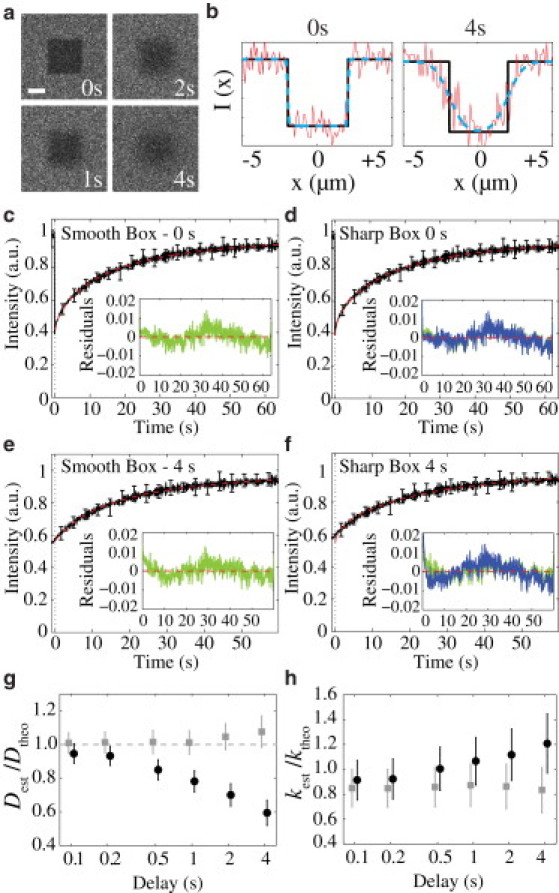
A smooth box (erf) model reduces errors associated with FRAP analysis compared to an ideal sharp box in FRAP simulations. (a) Output frames from simulations at the indicated times postbleach show how the bleach region changes with time. Scale bar = 2 μm. (b) Intensity plots for a 2-μm stripe in x across the bleached regions shown in panel a for bleach offsets of 0 or 4 s (red lines). Best fits based on smooth (dashed cyan lines) or sharp (black lines) boxes are indicated. (c–f) Mean FRAP recovery curves (black line ± SD) are shown along with the best fit (dashed red line) for either the smooth (c and e) or sharp (d and f) box regime for either a 0 s (c and d) or 4 s (e and f) bleach offset. Insets show residuals for the smooth box fit (green line) and sharp box fit (blue line). In panels d and f, the smooth box fits are underlaid to facilitate comparison. (g and h) Ratio of measured to theoretical input values for D and koff for varying bleach offset times (mean ± SE, n = 10) fit using the smooth (■) or sharp (●) box regimes. Note the smooth box regime yields similar measurements across all delay times.
Figure 4.
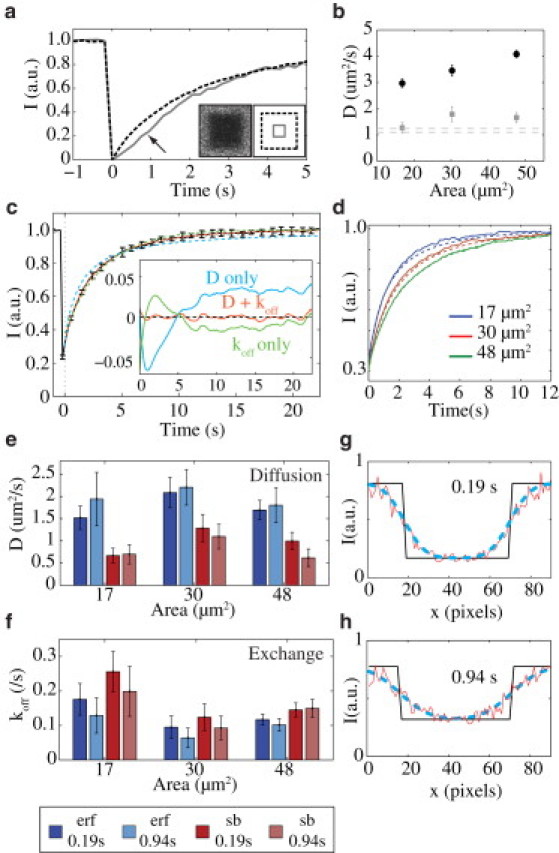
PHδ1 dynamics on the membrane are governed by a combination of lateral diffusion and membrane-cytoplasm exchange. (a) Mean intensity versus time within a square bleached region (dashed black line, Area = 48 μm2) or within a small box in the center of the bleached region (solid gray line) for a typical FRAP experiment after normalization such that I = 0 for the first postbleach frame (t = 0). Note the lag in recovery into the small central box (arrow). Inset shows a sample image of the first postbleach frame and the boundaries of the full (dashed black line) and central boxes (solid gray line). (b) Estimated diffusion coefficients (D, ± SE; n = 8) for bleached areas of three sizes fit with a pure lateral diffusion model (black circle) or the combined diffusion and exchange model (gray square) incorporating a one-frame (0.19 s) bleach offset. Dashed lines indicate previous measurements (11, 20). (c) Mean fluorescence intensity ± SD for a 48 μm2 bleach area (black line) and the accompanying fits using either a pure lateral diffusion model (cyan), a pure exchange model (green), or the combined diffusion and exchange model (red). t = 0 s is indicated (dashed vertical line). Residuals for the three models are shown in the inset using the same color code. (d) Experimental mean fluorescence intensity (solid lines) and the predicted recovery (dashed lines) for three bleach areas based on the measured recovery parameters in c: 17 μm2 (blue), 30 μm2 (red), and 48 μm2 (green). (e–f) Fit results for D and koff± SE (n = 8) for bleach areas of three different sizes with a 1 frame (0.19 s) or 5 frame (0.94 s) offset between bleaching and image analysis as fit with either the smooth box (erf) or sharp box (sb) functions. Results for the smooth box model are similar for both offset times. (g–h) Fluorescence profiles of GFP::PHδ1 (in x, red line) along a 20-pixel-wide line spanning the bleached region at 0.19 (e) or 0.94 s (f) after bleaching. Best fits using a sharp box (solid black line) and the smooth box (dashed cyan line) are shown. Note the smooth box fits the data significantly better in both cases.
The evolution of the membrane concentration as a function of time is then given by
| (9) |
For our purposes, we are interested in the mean fluorescence recovery within the bleached region given by
Normalization of individual FRAP curves to the prebleach steady-state values removes all dependence on kon∗. Solving the equation for the normalized mean fluorescence recovery within the bleach area for the initial condition specified by asmooth(x, 0) yields (see (18))
| (10) |
As formulated, the above solution reflects an accurate description for an infinitely long bleach stripe of width dx.
Extension to two-dimensional box geometry
We next consider a box-shaped bleach area (Fig. S1, C and F), centered at x, y = 0, with smooth edges. Analogously to Eq. 8, this geometry is described by
| (11) |
where
and i ∈ {x, y}, such that dx and dy describe the extent of the bleach region, and mx and my describe the slope of the fluorescence distribution at the edges of the ROI in the x and y directions, respectively. Note that by individually specifying the extent and the shape of bleaching along both axes, we also account for a potential anisotropy of the bleached region.
Following the logic for the one-dimensional case, the resulting normalized mean fluorescence recovery for a box-shaped bleach area centered at x, y = 0 is
| (12) |
where
| (13) |
and i ∈ {x, y}.
To obtain values for koff and D from fluorescent image data, the initial fluorescence distribution is fit with Eq. 11 to obtain values for mx, my, dx, and dy. For each frame, the fluorescence intensity is integrated from – dx/2 to dx/2 and – dy/2 to dy/2 to generate a recovery curve, which is then fit using Eq. 12 (see the Supporting Material).
Results and Discussion
Analysis of simulated FRAP datasets
To validate this approach, we tested its ability to accurately extract diffusion and detachment rates from computationally generated FRAP data sets for molecules characterized by differing diffusion and exchange rates under a variety of FRAP regimes using stochastic, particle-based simulations (see the Supporting Material).
Deviations from an ideal bleach geometry
We first analyzed the ability of this method to compensate for deviations from the ideal sharp box bleach geometry. In the simulations, we let bleaching occur only within a square bleach area, which for an immobile molecule would result in a bleached region that takes the form of a perfect square with sharp edges. However, lateral diffusion that occurs before image acquisition will smooth out these sharp edges, giving the apparent bleached region an altered shape.
To examine the effect of increasing time delays between bleaching and the first acquired image, which we define as the bleach offset, we generated a set of FRAP simulations for D = 0.1 μm2/s and koff = 0.01 s–1 and analyzed them beginning with various times postbleach. As shown in Fig. 1, a and b, increasing the bleach offset leads to a loss of sharp boundaries, with the effect increasing with increasing offset times. We compared the results obtained by fitting the anisotropic two-dimensional error function (smooth box, Eq. 11), with a two-dimensional version of Eq. 7 that describes a sharp-edged box (sharp box, Eq. S2 in the Supporting Material). For a 0 s offset, both functions fit the initial fluorescence distributions and yielded accurate estimates of both D and koff (Fig. 1, b–d, g and h). However, for increasing offset times, the sharp box no longer describes well the initial fluorescence and yields significant errors in the estimate of D and koff (Fig. 1, b, and f–h), whereas the smooth box continues to perform well with errors of <10% in D and <20% in koff for all offset times (Fig. 1, e, g, and h).
We also examined this case for changes in noise by repeating simulations with five- and 10-fold fewer particles. For no bleach offset, our fit regime yields accurate measurement of both D and koff across all noise levels, although the associated error increases (Fig. S2, A and B). At a 2 s bleach offset, the measured values begin to deviate from the theoretical values for the higher noise cases (Fig. S2, C and D). This effect appears to be due to difficulty in properly fitting the smoothening of the boundary (data not shown). However, despite this difficulty in fitting, it still generally results in better measurements, particularly for D, compared to the sharp box regime which fails to account for lateral diffusion during the offset (Fig. S2, C and D).
Deviations of the actual fluorescence distribution from that of a sharp-edged box can be induced by a variety of factors including, for example, molecules that diffuse at rapid timescales compared to bleach and image acquisition times. We examined two such conditions, increasing D relative to the frame capture rate, or increasing bleach duration, and found that the smooth box method was significantly better than the sharp box in both cases (Fig. S3), supporting the general applicability of this method and its advantage over a standard sharp box in extracting reasonable measures of diffusion and exchange kinetics.
Relative contributions of diffusion and exchange
We next examined the limits of this model in distinguishing the relative contributions of diffusion and exchange. If one process occurs significantly faster than the other, the contribution of the slower process may be masked. In such cases, the kinetic parameters obtained for the slower process may carry significant errors. To illustrate this effect, we examined the fits for D and koff obtained for simulations of a molecule diffusing at 0.1 μm2/s as koff was varied over several orders of magnitude (Fig. 2). We find that both parameters are well estimated within a range of values (0.001 < koff < 1 s–1). At higher values of koff, exchange dominates the behavior, masking the effects of diffusion, while at lower values, diffusion dominates (Fig. 2 a). The dependence of measured values on the relative timescales of diffusion and exchange is better visualized by plotting the ratio of measured to predicted values for koff and D as a function of the ratio of diffusive and exchange timescales (tD/tex). Fitting is reasonably accurate for both parameters (within a twofold range), provided this ratio remains with an order of magnitude of unity (Fig. 2 b). As one moves beyond this range, the recovery dynamics become increasingly dominated by one or the other process for a given bleach area (here 4 μm2). Therefore, when performing such FRAP experiments with a molecule of interest, it is important to choose a bleach box size that allows a suitable ratio between the timescales of recovery through diffusion and exchange. As will be discussed below, this requires performing the appropriate initial experiments to determine whether the implemented model and bleach area is suitable for a given system.
Figure 2.
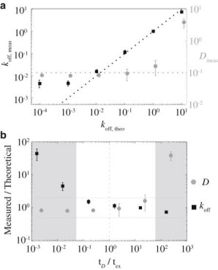
Distinguishing the effects of diffusion versus exchange. Simulations were performed (n = 6) for a broad range of exchange rates for Dtheo = 0.1 μm2/s. Measured values ± SE for koff (black squares) and D (gray circles) were obtained by fitting the simulation data for each value of koff, theo. In panel a, the measured values are plotted versus the input values for koff. Note that the measured values for koff fall along the predicted line (black dotted lines) over several orders of magnitude, but deviate significantly for koff < 10−2 s–1, a regime in which diffusion dominates. Similarly, measured values for D match the predicted value (gray dotted lines) until koff exceeds ∼1 s–1, when exchange begins to dominate. This pattern can be visualized better in panel b where the ratio between measured and theoretical values (Meas/Theo) is plotted as a function of the ratio of the diffusive and exchange timescales (tD = L2/2D, tex = koff–1, where L is half the edge width of the bleached square). For tD/koff between 0.1 and 10, reflecting reasonable balance between the processes of diffusion and exchange, both parameters are measured accurately. Beyond these limits (shaded regions), the dominance of one or the other process only allows accurate measurements of the dominant process. (Horizontal lines indicate a measured/theoretical ratio between 0.5 and 1.5. Vertical dotted line indicates tD/tex = 1.0.)
Effects of a cytoplasmic pool
The three-dimensional geometries of cells often present challenges for FRAP analysis. For photobleaching experiments on membrane-associated molecules, the effect of the soluble cytoplasmic pool of molecules beneath the membrane, which is typically also bleached, must be considered (Fig. 3 a). This is particularly true for the geometry considered in this work in which the bleach laser is perpendicular to the membrane. Because diffusion in the cytoplasm is typically faster than on the membrane, not accounting for this population can lead to artificially inflated estimates of D. This effect can be moderated by taking advantage of the distinct timescales of these two recoveries. If cytoplasmic recovery is significantly faster than recovery on the membrane, inclusion of a delay between the end of bleaching and the first analyzed frame (a bleach offset) will allow the cytoplasm to equilibrate and assume a homogeneous concentration. The analyzed curve will then primarily reflect the slower dynamics on the membrane. However, as we show above, incorporating this offset requires taking account of changes in the fluorescence distribution due to lateral diffusion.
Figure 3.
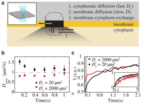
Effect of cytoplasmic diffusion on measurements of membrane recovery kinetics. (a) Schematic of bleaching geometry. Because of the extent of the point spread function of confocal microscopes typically used in FRAP, bleaching of a membrane will typically result in bleaching of the cytoplasm, particularly for the case depicted here in which the bleach laser is orthogonal to the membrane. Note that processes 1–3 may occur at different timescales, allowing them to be separated. (b) Values mean ± SE are shown (n = 10) for FRAP simulations incorporating cytoplasmic diffusion with Dc = 20 D (black square) or Dc = 2000 D (red square). Note the measured value for D in the former case (black square) approaches the theoretical value (D = 1 μm2/s) as the lag is increased to ≈0.4–0.8 s. In the latter case, all cytoplasmic recovery occurs between 0 and 0.1 s and no overestimation of D is seen. (c) Mean FRAP recoveries for the two cases in panel b. Note that for Dc = 2000 D (red line), there is a rapid phase of recovery due to the rapidly diffusing pool that occurs before the first imaged frame (shaded region t < 0.1 s). In contrast, for Dc = 20 D (black line) this rapid phase extends past t = 0.1 s and overlaps significantly with the membrane recovery. The two curves converge at approximately half a second, the time at which the measured values of D converge. (Inset) The two curves are normalized such that I (a.u.) = 0 at t = 0.1 s. Because of the contribution of the fast diffusing pool to the recovery, the black curve appears to recover faster than the red curve where only the slow-diffusing membrane associated pool is contributing to the recovery.
To illustrate this phenomenon, we performed simulations in which a molecule exchanges (koff = 0.1 s) between a slow diffusing state (membrane-associated, D = 1 μm2/s) and a rapid diffusing state (cytoplasmic, Dc = 20 D) with roughly 50% of molecules in each state at any given time. While this model ignores the complexity provided by three-dimensional diffusion, it is sufficient to illustrate how choosing a relatively arbitrary starting point for analyzing FRAP recovery curves, which is enabled by the smooth box fitting regime, allows separation of processes with distinct timescales.
If we fit the resulting simulations beginning with the first postbleach frame to extract a single diffusion constant, the rapid recovery by molecules in the fast-diffusing state leads to a significant overestimation of the slower, membrane-associated diffusion constant (Fig. 3 b, black squares, Time = 0.1 s). If we instead incorporate a bleach offset to allow molecules in the rapidly diffusing state to equilibrate, this overestimation declines significantly. In this case, introducing a lag of four frames (0.4 s) is sufficient to reduce this error to <20%. If we choose a significantly higher cytoplasmic diffusion rate (Dc = 2000 D), the recovery of the rapidly-diffusing species is complete before the first postbleach frame. As a result, the analyzed recovery is due primarily to the slow diffusing species and yields a membrane-associated diffusion constant that is accurate even if analysis begins with the first postbleach frame (Fig. 3 b, red squares). Notably, if one overlays the FRAP curves in the two cases, one can see that the two curves converge at ∼0.5 s, suggesting that at this offset, the contribution of cytoplasmic recovery in the case of Dc = 20 D becomes negligible (Fig. 3 c).
Experimental validation
A good candidate for testing the method described in this work is the plextrin-homology domain of PLCδ1 (PHδ1). This protein domain is known to bind phosphatidylinositol 4,5-bisphosphate (PIP2) and in most systems examined binds predominantly to the plasma membrane. It was recently shown this domain undergoes both rapid membrane-cytoplasm exchange and lateral diffusion when bound to the plasma membrane (11). Here we examine the behavior of a GFP-fusion to this domain within the Caenorhabditis elegans embryo (19). By slightly compressing the embryo on a glass coverslip, one can image an ∼20 × 20-μm area by confocal microscopy. Thus, it is relatively straightforward to bleach a two-dimensional square area within the plasma membrane.
Before proceeding with a comprehensive analysis using our method, we first confirmed that the behavior of PHδ1 in the C. elegans embryo is similar to that reported in mammalian cells, and that both lateral diffusion and membrane-cytoplasmic exchange were contributing significantly to fluorescence recovery at the length scales of our FRAP experiments. We first looked for evidence of lateral diffusion. For a square bleach area in a two-dimensional membrane, lateral diffusion can be detected in two ways.
First, recovery at the edges should precede that in the center. A plot of the normalized recovery of the entire box, compared to a box in the center of the bleach region, shows that the center of the bleach region exhibits a pronounced lag in the fluorescence recovery (Fig. 4 a, solid versus dashed lines).
Second, because an overall increase in the bleach area typically corresponds to an increase in the distance that unbleached molecules must diffuse to repopulate the bleached region, large bleach areas will generally require longer times for recovery. When we compare bleach areas of three distinct sizes, we find that recovery time increases with the area bleached (Fig. 4 d, solid lines). Thus, PHδ1 diffuses laterally when associated with the plasma membrane of the C. elegans embryo.
We next looked for evidence of membrane-cytoplasmic exchange, because PHδ1 is known to bind and unbind the plasma membrane on the order of seconds in mammalian cells. For the case where both lateral diffusion and membrane-cytoplasmic exchange contribute to the recovery, the relative contributions of the two processes will vary with the size of the bleach area. Specifically, as the bleach area becomes larger, there will be an increasing contribution of exchange to the overall recovery, which, if analyzed using a pure diffusion model, will yield artificially high diffusion rates. We analyzed FRAP areas of three sizes using Eq. 13 either fitting for D and koff or fixing koff at 0 s−1and fitting only for D. Fig. 4 b shows that a simple model of recovery by lateral diffusion yields an apparent diffusion constant that increases with bleach area, indicating that another process, most likely membrane-cytoplasmic exchange, is contributing to the observed recovery. This is very different from the case of pure diffusion. For example, analysis of soluble GFP confined within a pseudo two-dimensional geometry yields near-identical values for D, regardless of the size of the bleach area or whether a diffusion or diffusion-plus-exchange model is used (Table S1).
To extract the kinetic parameters using the full model, we obtained a series of FRAP curves for a square of edge-length 6.9 μm. After individually fitting initial postbleach frames and obtaining normalized fluorescence recovery curves for each experiment, we averaged the data and fit using Eq. 13 (Fig. 4 c), which yielded D = 1.7 ± 0.22 μm2/s and koff = 0.12 ± 0.016 s–1. In comparison, neither a diffusion-only or exchange-only model fit the data well, which can be seen in the plots of the residuals for the three cases. Using the coefficients obtained by fitting the full model, we could reproduce the recoveries observed for bleach areas of other sizes, which differ in the relative contributions lateral diffusion and exchange. As seen in Fig. 4 d, the recoveries for both areas are well predicted by these coefficients. If we instead fit each bleach area individually, the values we obtain for D and koff are similar across all three areas (Fig. 4, e and f). Together these results suggest that our two-component model captures well the dynamics of PHδ1.
The values of D we obtain are consistent with previous reports using FRAP and fluorescence correlation spectroscopy (Fig. 4, e and f, compare (11,20)), and differ from prior FRAP experiments using a pure diffusion model (21). This latter case coincidently yielded values that are close to the values we obtain when fitting a pure lateral diffusion model (Fig. 4 b). This highlights the importance of performing initial experiments to define properly the appropriate recovery model for analyzing FRAP data, including identifying the kinetic behaviors exhibited by a molecule and choosing the appropriately sized bleach area to interrogate those behaviors.
Our value for koff is of the same order of magnitude, but smaller than that reported by Hammond et al. (11), suggesting a somewhat longer lifetime on the membrane (∼7 s vs. 2.44 s). This could be due to differences in either the system (worm versus human) or the PH constructs used (rat versus human). However, this difference could also be due to differences in the FRAP geometries and analysis. Hammond et al. (11) bleach a Gaussian spot in a membrane oriented perpendicular to the imaging plane. By assuming that bleaching extent in Z is much greater than in X and Y, FRAP analysis can be simplified to a one-dimensional problem analogous to Eq. 10, which describes stripe bleaching. We do not know the height of the cells used, but HEK cells are likely to be 10 μm or less in height. Given that width of the Gaussian spots used are on the order of the height of the cells (5–10 μm), a size which is likely necessary to observe the effects of membrane-cytoplasmic exchange, it is possible that recovery in Z could be influencing their measurements, an effect to which our two-dimensional model would not be subject.
However, compared to Hammond et al. (11), our two-dimensional geometry is more susceptible to effects arising from the bleaching and recovery of the cytoplasmic pool below the membrane, which could, in principle, affect our measurements. To examine this possibility, we first bleached similar-sized bleach areas in the cytoplasm of embryos to establish the timescale of cytoplasmic equilibration. Recovery was extremely rapid (τ1/2 < 1 s, Fig. S4), consistent with measurements using fluorescence correlation spectroscopy (20). Coupled to the significantly higher fluorescence on the membrane compared the cytoplasm and short bleach times, the effects of this pool are likely small (see the Supporting Material). To verify that cytoplasmic recovery is not influencing our measurements, we included a bleach offset of ∼1 s to allow for cytoplasmic equilibration. As seen in Fig. 4, e and f, this offset does not significantly affect the values for D and koff, indicating that the effects of the cytoplasmic pool are negligible. It is worth pointing out that we are able to perform this analysis due to the use of our method to account for the effects of rapid lateral diffusion of PHδ1 during the bleach-offset period, which would otherwise tend to introduce errors. In this specific case, the initial fluorescence is less well described by a sharp-edged box (Fig. 4, g and h), and fits using this regime yielded significantly differing measurements, particularly after incorporating a ∼1 s bleach offset (Fig. 4, e and f).
Conclusion
While FRAP presents a robust, easily implemented and minimally invasive method for measuring the mobility of molecules within their native environments, obtaining quantitative estimates of a molecule's kinetic parameters requires suitable analytical and numerical analysis for properly analyzing FRAP experiments. Here we present an analytical solution for the case of a molecule undergoing reversible membrane association and lateral diffusion for two simple bleach geometries: a one-dimensional stripe and a two-dimensional box, bleached onto the surface of a membrane. Compared to typical assumptions of ideal sharp-edged bleach geometries, this scheme involves taking an arbitrary postbleach frame and parameterizing the actual fluorescence distribution. This parameterization of both the extent of the bleach area and the smoothening of the boundaries allows for reconstruction of an accurate but analytically accessible representation of the molecule distribution. By fitting the fluorescence recovery using a kinetic model to describe the time evolution of this initial distribution, we can obtain accurate estimates for both membrane-cytoplasmic exchange and lateral diffusion. Notably, because this procedure takes into account deviations from the ideal bleach shape (here a box or stripe), it can account for a variety of factors that may limit the sharpness of the boundaries of the bleached region, including, but not limited to optical limitations or lateral diffusion of bleached and unbleached molecules during the preanalysis phase, which could otherwise induce significant errors.
Previous solutions for analyzing FRAP to extract diffusion and exchange rates of a reversibly membrane-associated molecule have been described for Gaussian spot bleach geometries (10,11), specifically for the one-dimensional case analogous to the smooth-edged stripe described by Eq. 10. Importantly, the advantages of our method typically also apply to the Gaussian bleach geometry: Both can be used for either one- or two-dimensional geometries, and both can account for deviations in the ideal bleach shape due to various effects, including lateral diffusion. Thus, the strategies we describe here, such as including a bleach offset, apply to both methods.
At the same time, both methods also share similar limitations. Bleaching within a two-dimensional planar configuration necessarily induces bleaching in the cytoplasm below the membrane and is subject to Z-drift, which must be taken into account in both cases. Shifting to a one-dimensional geometry in which the membrane to be bleached is orthogonal to the imaging plane reduces, but does not eliminate, these effects. However, the one-dimensional geometry introduces an added requirement that bleaching in Z significantly exceeds that in the X, Y plane. The contributions in the Z axis to recovery can then be neglected, enabling the use of one-dimensional model. This is usually accomplished through opening the pinhole to increase bleach depth, but there are limitations to this depth due to a variety of factors, such as sample depth or curvature.
Importantly, the implementation of either method to accurately measure diffusion and exchange requires interrogating a bleach area of the appropriate size. Specifically, measurement of exchange kinetics that are relatively slow relative to diffusion requires relatively large bleach areas. In this last respect, our method provides additional flexibility to a Gaussian spot, which, although also implementable on confocal systems, has several constraints. Achieving and fitting large Gaussian spots can be complicated by the tails of the fluorescence distribution. If these tails are truncated by the edges of the cell, errors are introduced. By contrast, achieving large areas is straightforward with a box, especially because the sharpness of the boundaries does not scale with box size. Finally, in considering two-dimensional bleach geometries, it is important to note that Gaussian spots are necessarily isotropic. In contrast, our method allows for anisotropies in shape (rectangles versus squares), which allows for bleach areas to be more easily adapted to cellular geometries.
Data analysis using our method for FRAP analysis is no more complicated than other standard bleach geometries, including Gaussian spots. The bleach areas we describe—simple boxes or stripes—are widely used and easily implemented on model confocal microscopes. It can be implemented on planar geometries such as we describe for PHδ1 in which a two-dimensional surface can be imaged, or for bleaching along a one-dimensional line such as a cell boundary using the one-dimensional stripe model (Eq. 10). Because fitting relies only on the initial distribution of fluorescence right after the bleaching process, it does not require specific information regarding the beam geometry, and it is robust to deviations of the initial postbleach frame due to delays in acquisition, increased bleach times, or physical limitations in the spatial resolution of the bleaching beam. This property allows for significant variations in experimental setups.
Finally, in practice, fitting FRAP experiments requires only two steps which are standard for most FRAP methods: First, the initial fluorescence distribution in the postbleach frame is fit to obtain the edge and slope parameters of the bleach region. Second, the fluorescence recovery in the area defined by these parameters is extracted and fit using standard curve fitting software. Much of this process can be automated with minimal user input. To facilitate use of this method, MATLAB scripts (The MathWorks, Natick, MA) for analyzing two-dimensional boxes are provided (see the Supporting Material).
In summary, the FRAP methodology we describe provides a relatively simple and robust method for measuring diffusion and exchange kinetics of molecules in a variety of biological contexts. It allows for accurate measurement of both lateral diffusion and membrane-cytoplasmic exchange under realistic conditions. It is also robust to delays between bleaching and image acquisition which may be either intrinsic to the experimental setup or incorporated to reduce the contribution of more rapid processes that would otherwise interfere with accurate analysis. Thus, we feel this method will prove useful in a wide variety of experimental contexts.
Acknowledgments
The authors thank J. Bois, A. Klopper, P. Khuc Trong, E. Paluch, and Z. Petrásek for critical comments on the manuscript. D. Drexel kindly provided recombinant GFP.
This work was supported by the Alexander von Humboldt Foundation and a Marie Curie Grant (No. 219286) from the European Commission (N.W.G.), and the Max-Planck Institute for the Physics of Complex Systems Visitor's Program (D.C.).
Footnotes
This is an Open Access article distributed under the terms of the Creative Commons-Attribution Noncommercial License (http://creativecommons.org/licenses/by-nc/2.0/), which permits unrestricted noncommercial use, distribution, and reproduction in any medium, provided the original work is properly cited.
Supporting Material
References
- 1.Rabut G., Ellenberg J. Photobleaching techniques to study mobility and molecular dynamics of proteins in live cells: FRAP, iFRAP and FLIP. In: Goldman R.D., Spector D.L., editors. Live Cell Imaging: A Laboratory Manual. Vol. 1. Cold Spring Harbor Laboratory Press; Cold Spring Harbor, NY: 2005. pp. 101–127. [DOI] [PubMed] [Google Scholar]
- 2.Sprague B.L., McNally J.G. FRAP analysis of binding: proper and fitting. Trends Cell Biol. 2005;15:84–91. doi: 10.1016/j.tcb.2004.12.001. [DOI] [PubMed] [Google Scholar]
- 3.Poo M., Cone R.A. Lateral diffusion of rhodopsin in the photoreceptor membrane. Nature. 1974;247:438–441. doi: 10.1038/247438a0. [DOI] [PubMed] [Google Scholar]
- 4.Liebman P.A., Entine G. Lateral diffusion of visual pigment in photoreceptor disk membranes. Science. 1974;185:457–459. doi: 10.1126/science.185.4149.457. [DOI] [PubMed] [Google Scholar]
- 5.Axelrod D., Koppel D.E., Webb W.W. Mobility measurement by analysis of fluorescence photobleaching recovery kinetics. Biophys. J. 1976;16:1055–1069. doi: 10.1016/S0006-3495(76)85755-4. [DOI] [PMC free article] [PubMed] [Google Scholar]
- 6.McNally J.G. Quantitative FRAP in analysis of molecular binding dynamics in vivo. Methods Cell Biol. 2008;85:329–351. doi: 10.1016/S0091-679X(08)85014-5. [DOI] [PubMed] [Google Scholar]
- 7.Soumpasis D.M. Theoretical analysis of fluorescence photobleaching recovery experiments. Biophys. J. 1983;41:95–97. doi: 10.1016/S0006-3495(83)84410-5. [DOI] [PMC free article] [PubMed] [Google Scholar]
- 8.Ellenberg J., Siggia E.D., Lippincott-Schwartz J. Nuclear membrane dynamics and reassembly in living cells: targeting of an inner nuclear membrane protein in interphase and mitosis. J. Cell Biol. 1997;138:1193–1206. doi: 10.1083/jcb.138.6.1193. [DOI] [PMC free article] [PubMed] [Google Scholar]
- 9.Coscoy S., Waharte F., Amblard F. Molecular analysis of microscopic ezrin dynamics by two-photon FRAP. Proc. Natl. Acad. Sci. USA. 2002;99:12813–12818. doi: 10.1073/pnas.192084599. [DOI] [PMC free article] [PubMed] [Google Scholar]
- 10.Oancea E., Teruel M.N., Meyer T. Green fluorescent protein (GFP)-tagged cysteine-rich domains from protein kinase C as fluorescent indicators for diacylglycerol signaling in living cells. J. Cell Biol. 1998;140:485–498. doi: 10.1083/jcb.140.3.485. [DOI] [PMC free article] [PubMed] [Google Scholar]
- 11.Hammond G.R.V., Sim Y., Irvine R.F. Reversible binding and rapid diffusion of proteins in complex with inositol lipids serves to coordinate free movement with spatial information. J. Cell Biol. 2009;184:297–308. doi: 10.1083/jcb.200809073. [DOI] [PMC free article] [PubMed] [Google Scholar]
- 12.Sprague B.L., Pego R.L., McNally J.G. Analysis of binding reactions by fluorescence recovery after photobleaching. Biophys. J. 2004;86:3473–3495. doi: 10.1529/biophysj.103.026765. [DOI] [PMC free article] [PubMed] [Google Scholar]
- 13.Weiss M. Challenges and artifacts in quantitative photobleaching experiments. Traffic. 2004;5:662–671. doi: 10.1111/j.1600-0854.2004.00215.x. [DOI] [PubMed] [Google Scholar]
- 14.Seiffert S., Oppermann W. Systematic evaluation of FRAP experiments performed in a confocal laser scanning microscope. J. Microsc. 2005;220:20–30. doi: 10.1111/j.1365-2818.2005.01512.x. [DOI] [PubMed] [Google Scholar]
- 15.Hauser G.I., Seiffert S., Oppermann W. Systematic evaluation of FRAP experiments performed in a confocal laser scanning microscope. Part II. Multiple diffusion processes. J. Microsc. 2008;230:353–362. doi: 10.1111/j.1365-2818.2008.01993.x. [DOI] [PubMed] [Google Scholar]
- 16.Beaudouin J., Mora-Bermúdez F., Ellenberg J. Dissecting the contribution of diffusion and interactions to the mobility of nuclear proteins. Biophys. J. 2006;90:1878–1894. doi: 10.1529/biophysj.105.071241. [DOI] [PMC free article] [PubMed] [Google Scholar]
- 17.Sprague B.L., Müller F., McNally J.G. Analysis of binding at a single spatially localized cluster of binding sites by fluorescence recovery after photobleaching. Biophys. J. 2006;91:1169–1191. doi: 10.1529/biophysj.105.073676. [DOI] [PMC free article] [PubMed] [Google Scholar]
- 18.Gradshteyn I.S., Ryzhik I.M. 7th Ed. Academic Press; New York: 2007. Table of Integrals, Series and Products. [Google Scholar]
- 19.Audhya A., Hyndman F., Oegema K. A complex containing the Sm protein CAR-1 and the RNA helicase CGH-1 is required for embryonic cytokinesis in Caenorhabditis elegans. J. Cell Biol. 2005;171:267–279. doi: 10.1083/jcb.200506124. [DOI] [PMC free article] [PubMed] [Google Scholar]
- 20.Petrásek Z., Hoege C., Schwille P. Characterization of protein dynamics in asymmetric cell division by scanning fluorescence correlation spectroscopy. Biophys. J. 2008;95:5476–5486. doi: 10.1529/biophysj.108.135152. [DOI] [PMC free article] [PubMed] [Google Scholar]
- 21.Brough D., Bhatti F., Irvine R.F. Mobility of proteins associated with the plasma membrane by interaction with inositol lipids. J. Cell Sci. 2005;118:3019–3025. doi: 10.1242/jcs.02426. [DOI] [PubMed] [Google Scholar]
Associated Data
This section collects any data citations, data availability statements, or supplementary materials included in this article.