Modeling the Effects of Subcutaneous Insulin Administration and Carbohydrate Consumption on Blood Glucose

Abstract

Background

Estimation of the magnitude and duration of effects of carbohydrate (CHO) and subcutaneously administered insulin on blood glucose (BG) is required for improved BG regulation in people with type 1 diabetes mellitus (T1DM). The goal of this study was to quantify these effects in people with T1DM using a novel protocol.

Methods

The protocol duration was 8 hours: a 1–3 U subcutaneous (SC) insulin bolus was administered and a 25-g CHO meal was consumed, with these inputs separated by 3–5 hours. The DexCom SEVEN® PLUS continuous glucose monitor was used to obtain SC glucose measurements every 5 minutes and YSI 2300 Stat Plus was used to obtain intravenous glucose measurements every 15 minutes.

Results

The protocol was tested on 11 subjects at Sansum Diabetes Research Institute. The intersubject parameter coefficient of variation for the best identification method was 170%. The mean percentages of output variation explained by the bolus insulin and meal models were 68 and 69%, respectively, with root mean square error of 14 and 10 mg/dl, respectively. Relationships between the model parameters and clinical parameters were observed.

Conclusion

Separation of insulin boluses and meals in time allowed unique identification of model parameters. The wide intersubject variation in parameters supports the notion that glucose-insulin models and thus insulin delivery algorithms for people with T1DM should be personalized. This experimental protocol could be used to refine estimates of the correction factor and the insulin-to-carbohydrate ratio used by people with T1DM.

Introduction

The presentation of knowledge of the dynamic behavior of a system may take a variety of forms, e.g., flowcharts with logical statements, or sets of mathematical equations. The decision on how to present this information depends upon the purpose of the model, and who needs to understand the model. In the case of glucose-insulin models, the purpose of the model can be for measurement, simulation, prediction, and control.¹ The people who need to understand the model range from scientists and engineers to physicians and people with diabetes mellitus.

Physicians treating people with type 1 diabetes mellitus (T1DM) are modeling in order to improve glycemia. Over the course of therapy, a patient with T1DM will be assigned a correction factor (CF) and an insulin-to-carbohydrate ratio (ICR). The person with diabetes will attempt to regulate their blood glucose (BG) using the CF and ICR, along with additional dynamic information available in the form of insulin-on-board (IOB) decay curves,² which may be used by their insulin pump to recommend an insulin bolus size.³ When used properly, these clinical parameters are sufficient for reducing the prevalence of diabetic complications.⁴

Given the difficulty in maintaining successful open-loop control and the development of continuous glucose monitoring (CGM) sensors and continuous subcutaneous insulin infusion (CSII) pumps, new models have been developed for control.¹ Studies have used nonlinear models developed using tracers and intravenous (IV) measurements.^5–8 Personalization of these models is expensive and not practical to extend to all people with T1DM. Minimal models have been considered, but may require IV measurements.^9–11 Empirical models using only subcutaneous (SC) glucose, insulin delivery, and carbohydrate (CHO) records have been investigated^12,13 and have also been used as the basis for closed-loop control algorithms in clinical trials.¹⁴ The unique identification of parameters from ambulatory data is problematic due to the nature of the data itself: people with T1DM often take boluses and meals simultaneously; simultaneous input excitation may lead to incorrect sign of gain from a statistically optimal parameter estimate.¹⁵ As such, these empirical models need further heuristics to ensure that they are suitable for their intended purpose.

A nonlinearity assessment has suggested that adequate control of BG can be obtained using linear methods.¹⁶ An application such as closed-loop insulin delivery requires an interdisciplinary approach to the development of a functional device. In this article, we therefore propose a linear model with a small number of clinically meaningful parameters to approximate this complex, nonlinear process. A novel clinical trial was implemented in order that the model parameters could be uniquely identified. The relationship between the model parameters and clinical parameters was then revealed.

Methods

Experimental Protocol

Clinical data were obtained from 11 adult subjects with T1DM, 6 females and 5 males, using protocol approved by the Institutional Review Board at the Sansum Diabetes Research Institute, Santa Barbara, CA. Informed, witnessed consent was obtained from subjects. Eleven sets of data were obtained.

Subjects began the experiment under conditions assumed to be steady state, i.e., no insulin boluses, basal changes, or meals within at least the last four hours. The two inputs considered were a test meal and an insulin bolus; these inputs were not given simultaneously. The order in which the inputs were given was dependent upon arrival conditions and safety considerations. After the test meal was consumed, no bolus or basal changes were made in at least the next two hours. After the bolus was administered, no meals were consumed or basal changes made in at least the next three hours.

The test meal was a mixed meal with 25-g CHO, and was identical for each subject. The insulin bolus was 1–3 U, depending upon the subject's ICR, CF, and latest glucose measurement, and was administered using the subject's CSII pump. The size of these inputs was chosen such that symptomatic hypoglycemia and hyperglycemia would be avoided during the experiment. It is important to note that no insulin bolus was given at the time of meal ingestion. The insulin bolus was only given to correct for the elevated BG after conditions corresponding to steady state were obtained.

The subject's CF and ICR were obtained before the experiment. Data collected during the experiment consisted of YSI 2300 Stat Plus (Yellow Springs Instruments, Yellow Springs, OH) IV glucose measurements every 15 minutes, and DexCom SEVEN® PLUS (DexCom, San Diego, CA) SC glucose measurements every 5 minutes.

Model Structure

The model type was a continuous time transfer function consisting of a component for modeling SC insulin effects and another component for modeling CHO effects on BG. Transfer functions are a powerful engineering tool used to reduce the relatively complex properties and solution of ordinary differential equations (ODEs) to the simpler solution process associated with algebraic equations (AEs). The time domain variable, t, is replaced with the frequency (or Laplace) domain variable, s, and standard transformations of ODEs into AEs exist in the scientific literature.¹⁷ The structure of each component was first order plus time delay with integrator. The first component, the model of bolus insulin effects on BG, was

$${\Upsilon }_B(s)=\frac{K_{B}exp(-{\theta }_{B}s)}{s({\tau }_{B}s+1)}{u}_B(s)$$ (1)

where s is the Laplace variable, Y_B is the deviation BG due to bolus insulin, and U_B is the insulin delivery. The second component, the model of meal CHO effects on BG, was

$${\Upsilon }_M(s)=\frac{K_{M}exp(-{\theta }_{M}s)}{s({\tau }_{M}s+1)}{u}_M(s)$$ (2)

where Y_M is the deviation BG due to meal CHO, and U_M is the meal CHO amount. K is the model gain, τ is the model time constant, and θ the model time delay for bolus insulin and meal CHO effects denoted by subscripts B and M, respectively. The model components described in Equation (1) and Equation (2) are summed to give the complete model, which is

$$\Upsilon (s)={\Upsilon }_B(s)+{\Upsilon }_M(s)$$ (3)

where Y is the deviation BG due to both bolus insulin and meal CHO effects.

Parameter Estimation

The model parameters K, τ and θ were estimated using heuristics and least-squares optimization.^17,18 The heuristics used to estimate each parameter were as follows:

1. K was the ratio of the greatest deviation of the output y(t) from steady state to the magnitude of the deviation of the input u(t) from steady state, thus

   $$K=\frac{y_{max}-y_{ss}}{u_{max}-u_{ss}}$$ (4)

2. θ was defined as the time at which y(t) first exceeded 3% of its maximum response subject to the input u(t), thus

   $$y(t=\theta ) = 0.03u_{max}$$ (5)

3. τ was defined as the time at which y(t) first attained 63.2% of its maximum response subject to the input u(t), thus

$$y(t=\tau +\theta ) = 0.632K{u}_{max}$$ (6)

These rules are summarized graphically in Figure 1, where a system is subject to a unit impulse input at time zero. In this example, there is no measurement noise, and thus there is no output change until time θ has passed. Also, note that if the input had magnitude other than unity, i.e., M = u_max – u_ss, then the final output response would be KM = y_max – y_ss.

Figure 1.

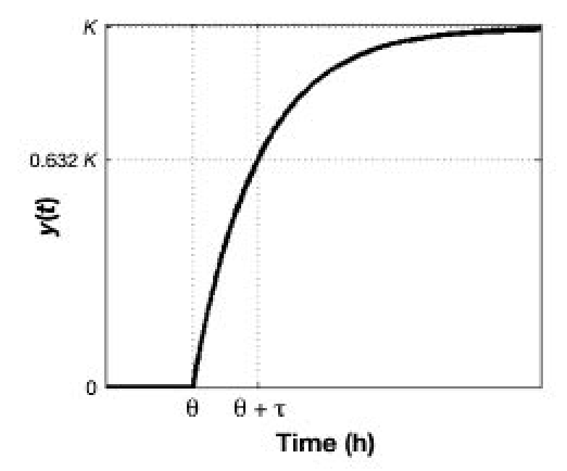
Diagram showing how parameters K, τ, and θ are determined using heuristics from the output response y(t) to a hypothetical unit impulse at time zero to an integrating system.

Performance Metrics

The FIT metric was used to quantify the model performance, and is defined as:

$$FIT(\%)=100\left(1-\frac{\sum _{i=1}^n|y_i-{\widehat{y}}_i|}{\sum _{i=1}^n|y_i-{\overline{y}}_i|}\right)$$ (7)

where i is the sample index, n is the number of samples, y_i is the BG measurement, ŷ_i is the model estimate of BG, and ŷ is the mean BG measurement. The FIT metric corresponds to the percentage of the variation in the data explained by the model; a perfect FIT is 100%, while a value of 0% implies that equivalent model performance would be attained by predicting the mean measurement value. The root mean square error (RMSE) was also used, defined as

$$RMSE=\sqrt{\frac{\sum _{i=1}^n{(y_i-{\widehat{y}}_i)}^2}{n}}$$ (8)

Relationship between Model Parameters and Clinical Parameters

Dimensional analysis of the model gains, K, indicated relationships with the clinical parameters CF and ICR. The insulin bolus model gain, K_B, has units of [(mg/dl) per U], which is equivalent to those of the CF, which is the drop in BG from one unit of rapid-acting insulin, thus

$$K_B=-CF$$ (9)

The meal model gain, K_M, has units of [(mg/dl) per g CHO]. ICR, which is the amount of CHO compensated for by one unit of rapid-acting insulin is usually expressed as a ratio of units of insulin to g CHO, which as a decimal would have units of [U per (g CHO)]; the product of CF and ICR has units of [(mg/dl) per g CHO], thus

$$K_M=CF\cdot ICR$$ (10)

Results

Clinical Data

Table 1 summarizes the implementation of the protocol carried out on the 11 subjects. For subject 2, no CGM data were available due to CGM failure. For subjects 4, 5, and 6, no YSI data were available due to occlusion of the IV line. The CGM and venous plasma glucose assessed using the YSI data were compared using the point error grid analysis (pEGA)¹⁹ and rate error grid analysis (rEGA).²⁰ According to pEGA, shown in Figure 2, 99% of data pairs were in regions A and B, where A indicates accurate, and B indicates benign. According to rEGA, shown in Figure 3, 97% of data pairs were in regions A and B.

Table 1.

Summary of Data Collected from Protocol for Each Subject

Subject	Start time of data	YSI data		CGM data		First impulse	Response duration (min)
		Bolus	Meal	Bolus	Meal		Bolus	Meal
1	9:30 AM	Yes	Yes	Yes	Yes	Meal	300	130
2	9:30 AM	Yes	Yes	No	No	Meal	300	130
3	9:25 AM	Yes	Yes	Yes	Yes	Meal	285	130
4	8:15 AM	No	Yes	Yes	Yes	Bolus	210	210
5	9:25 AM	No	Yes	Yes	Yes	Meal	225	135
6	8:45 AM	No	Yes	Yes	Yes	Meal	315	180
7	9:40 AM	Yes	Yes	Yes	Yes	Bolus	150	210
8	9:20 AM	Yes	Yes	Yes	Yes	Bolus	195	120
9	8:40 AM	Yes	Yes	Yes	Yes	Bolus	195	120
10	9:10 AM	Yes	Yes	Yes	Yes	Bolus	195	180
11	9:05 AM	Yes	Yes	Yes	Yes	Bolus	210	195

Figure 2.

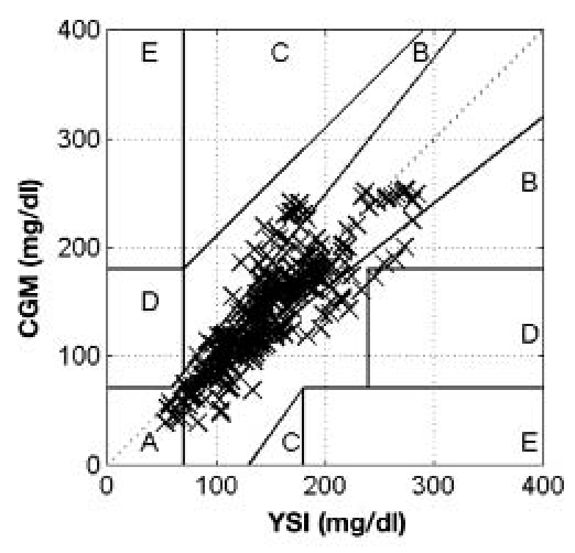
Summary of YSI and CGM data collected from all trials using the point error grid analysis.¹⁹ Points were distributed as follows: 76% zone A, 23% zone B, 0% zone C, <1% zone D, 0% zone E.

Figure 3.

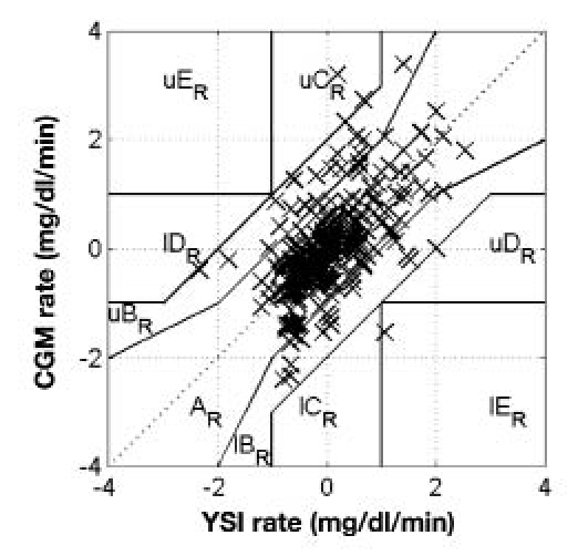
Summary of YSI and CGM data collected from all trials using the rate error grid analysis.²⁰ Prefix l indicates lower, prefix u indicates upper. Subscript R indicates rate. Points were distributed as follows: 78% zone A_R, 21% zone B_R, 2% zone C_R, < 1% zone DR, < 1% zone E_R.

The data collected for subjects 1–11 are shown in Figure 4 and Figure 5. These results show that there is often a disparity between YSI and CGM measurements, whether at low or high BG. Also, high frequency noise in CGM measurements for subject 3 and subject 8, along with CGM failure in subject 2 indicate that CGM devices are not as reliable as manual YSI measurement. Table 2 summarizes analysis of bias in the comparison of YSI and CGM data. Using a paired t-test at the 95% significance level, there was no absolute bias in 8 out of 10 data sets, increasing to 9 out of 10 at the 99% significance level. Four out of 10 data sets showed no evidence of a nonzero intercept and nonunity slope at the 95% significance level, increasing to 6 out of 10 at the 99% significance level.

Figure 4.

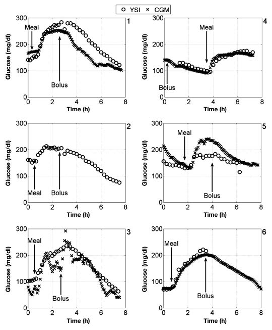
Glucose data for subjects 1–6, with meal consumption and bolus administration indicated relative to experimental time.

Figure 5.

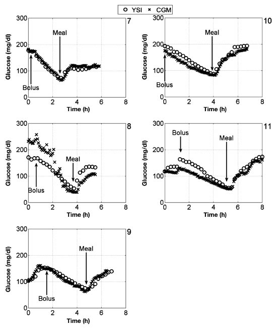
Glucose data for subjects 7–11, with meal consumption and bolus administration indicated relative to experimental time.

Table 2.

Statistical Analysis of Bias between YSI and CGM Data Collected^a

Subject	Absolute bias		Nonzero intercept		Nonunity slope
	95%	99%	95%	99%	95%	99%
1	Yes	No	Yes	No	No	No
2	N/A	N/A	N/A	N/A	N/A	N/A
3	No	No	Yes	Yes	Yes	Yes
4	No	No	Yes	No	No	No
5	Yes	Yes	Yes	Yes	Yes	Yes
6	No	No	No	No	Yes	No
7	No	No	No	No	Yes	No
8	No	No	Yes	Yes	Yes	Yes
9	No	No	Yes	Yes	Yes	Yes
10	No	No	No	No	No	No
11	No	No	No	No	No	No
No bias (% of data sets)	80	90	40	60	40	60

^aAbsolute bias was based on a paired two-tail t-test, intercept and slope bias was based on confidence intervals of the regression line. Percentages given are significance levels.

Model Parameters

Six parameters were identified for each data set. The mean parameter values and coefficient of variation for each identification method and data set are given in Table 3. For the bolus insulin model, the mean of the gains and time constants identified from YSI and CGM data using optimization were three to four times greater than the corresponding parameters identified from heuristics. The coefficient of variation for the gain and time constant from the bolus insulin model obtained using optimization was greater than 100%. The meal CHO model parameters differed by less than a factor of two for each set of data and method used.

Table 3.

Summary of Mean (Coefficient of Variation %) of Model Parameters Obtained through Heuristics and Optimization from YSI and CGM Data

Parameter	Heuristics		Optimization
	YSI	CGM	YSI	CGM
KB (mg/dl per U)	−95(33)	−72(66)	−320(88)	−270(160)
τB (min)	150(22)	110(32)	550(80)	440(100)
θB (min)	6.4(120)	33(170)	53(230)	31(160)
KM (mg/dl per g CHO)	3.6(40)	3.5(34)	3.9(46)	3.5(39)
τM (min)	59(34)	41(52)	48(71)	37(88)
θM (min)	10(92)	21(79)	12(59)	22(72)

Comparison of Model Parameters with Clinical Parameters

The bolus insulin model gains and the subject's CF are compared in Figure 6. The bolus insulin model gains identified using heuristics lie closer to the 45° line than those identified by optimization. The meal CHO model gains and the product of the subject's CF and ICR are compared in Figure 7. Both identification methods show similar results. The correlation coefficients, r, were calculated and a hypothesis test was performed to determine the statistical significance of any correlation between these parameters. The null hypothesis was that there was no correlation. The correlation coefficients and p values for each correlation are shown in Table 4. The range of correlation coefficients was 0.7–65%. In each case, the p value was greater than .05, thus the null hypothesis was not rejected, so at the 95% significance level there was no correlation between K_B and CF, and K_M and CF·ICR.

Figure 6.

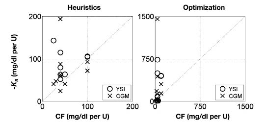
Comparison of the clinical parameter CF with the experimentally determined gain K_B from both YSI and CGM data. Left: parameters determined from heuristics. Right: parameters determined from optimization. Note different axis scaling.

Figure 7.

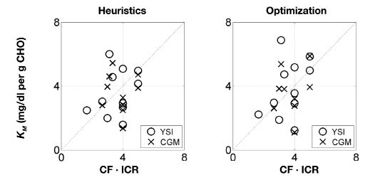
Comparison of the product of the clinical parameter CF and ICR with the experimentally determined gain K_M from both YSI and CGM data. Left: parameters determined from heuristics. Right: parameters determined from optimization.

Table 4.

Summary of Correlation Coefficients and p values for Hypothesis Test of Nonzero Correlation between Clinical Parameters CF and ICR and Estimated Model Parameters K_B and K_M Obtained through Heuristics and Optimization from YSI and CGM Data.

Method	Data type	−KB vs CF		KM vs CF·ICR
		r (%)	p	r (%)	p
Heuristics	YSI	65	.081	33	.33
Heuristics	CGM	14	.7	36	.3
Optimization	YSI	0.7	.99	41	.21
Optimization	CGM	15	.68	27	.44

Figure 8 compares the normalized BG response of the bolus insulin models identified using heuristics with a range of nonlinear IOB decay curves of 2–8 hours.² The five-hour IOB decay curve lies within the range of the normalized responses of the bolus insulin models developed from YSI and CGM data. Figure 9 compares the normalized BG response of the meal CHO models identified using heuristics with the normalized glucose absorption amount from the meal CHO model presented by Hovorka and colleagues.²² The normalized glucose absorption response amount lies within the range of the normalized responses of the meal CHO models developed from YSI and CGM data.

Figure 8.

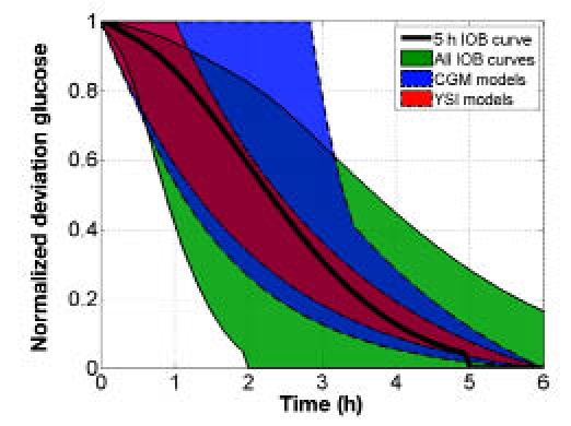
Comparison of the range of normalized bolus insulin model glucose responses to insulin from IOB curves,² where the bolus insulin model dynamics were identified from heuristics from YSI and CGM data.

Figure 9.

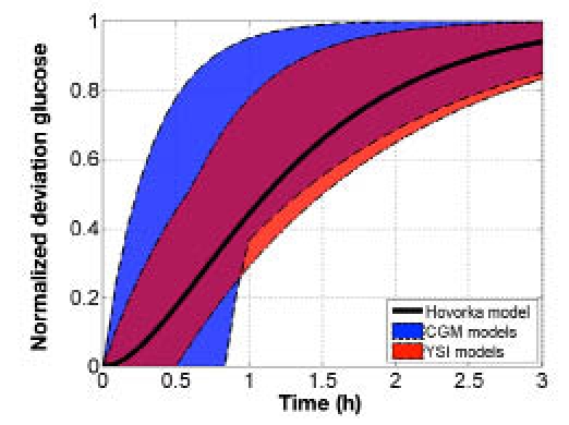
Comparison of the range of normalized meal CHO model glucose responses to CHO with Hovorka meal model response,²¹ where the meal CHO model dynamics were identified using heuristics from YSI and CGM data.

Model Performance

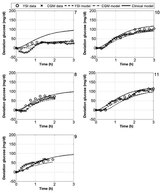
The bolus insulin response and model outputs for subjects 1–11 are shown in Figure 10 and Figure 11. The models derived from CGM and YSI data with parameters identified from heuristics models capture the low frequency characteristics of the data over a five-hour window better than the clinical model based upon the subject's correction factor and five-hour IOB decay curve. The meal response and model outputs for subjects 1–11 are shown in Figure 12 and Figure 13. The model derived from clinical parameters and the Hovorka meal response characteristic captured the low frequency characteristics over the three-hour time span. The model performance was assessed using the FIT metric (Figure 14) and the RMSE value (Figure 15).

Figure 10.

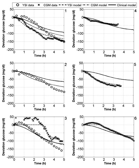
Deviation glucose data and models for subjects 1–6, where a 1 U insulin bolus was administered at time 0.

Figure 11.

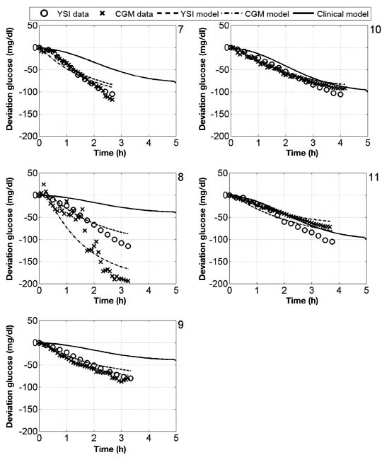
Deviation glucose data and models for subjects 7–11, where a 1 U insulin bolus was administered at time 0.

Figure 12.

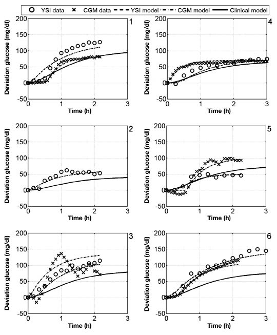
Deviation glucose data and models for subjects 1–6, where a 25 g CHO was administered at time 0.

Figure 13.

Deviation glucose data and models for subjects 7–11, where a 25 g CHO was administered at time 0.

Figure 14.

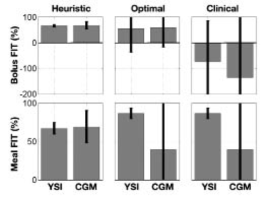
Mean and standard deviation of the FIT metric for each model, derived from both YSI and CGM data, based on heuristics, optimization, and clinical parameters.

Figure 15.

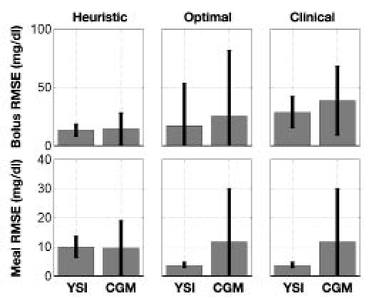
Mean and standard deviation of the RMSE metric for each model, derived from both YSI and CGM data, based on heuristics, optimization, and clinical parameters.

Discussion

The protocol designed was simple to execute; the most challenging aspect was the use of an IV line for IV blood samples for the YSI. The YSI and CGM data were strongly correlated, as shown by the pEGA and rEGA analysis, indicating that the experiment may be implemented reliably without any IV samples to obtain similar results. There were noticeable differences in YSI and CGM samples, such as offset and a lead/lag of one measurement against another; however, these differences were not consistent, and according to the pEGA and rEGA, these differences were not clinically significant. However, when considering bias through statistical methods, although there was little evidence in support of absolute bias, there was evidence that half of the data sets showed significant bias in terms of slope and intercept of the regression line. These biases then led to differences between the parameters that were estimated from CGM and YSI measurements. This could be because of the lead/lag between venous blood glucose and interstitial fluid glucose, or because of unreliable sensors. Without a gold standard measurement for SC glucose, it is not possible to determine which was the case.

The main assumption underlying the validity of the models and parameter estimates was “steady state.” Although steady state does not exist in a mathematical sense, it does exist in a practical sense. In this case, steady state meant a clinical judgment on when the rate of change of BG was less than it would have been due to meal CHO or bolus insulin.

The comparison of clinical and model parameters indicated a disparity between the two, but did not indicate one parameter being more valid than any other in a general sense. The model parameters fit the data better, but given that the clinical parameters may have been developed from more data, the clinical parameter could be more appropriate for any future day. Although the clinical parameter appears to have the same units and the model parameter, the manner in which the parameter is determined would affect the value, i.e., was it developed with an engineering definition of steady state in mind, or was it developed with the objective of a return to euglycemia as fast as possible? In the case of the latter, the occurrence of hypoglycemia may be prevalent without a small compensatory snack.

The comparison of the model dynamics with those of IOB and the Hovorka glucose absorption amount showed that these published dynamics were comparable to the models developed from these clinical data. Although there were intersubject variations, the critical low and high bandwidth frequencies of the responses were captured.

The model proposed in this article was conceived for a very different purpose than those models developed from tracer experiments.^5–7 These prior works have yielded excellent simulation models for testing insulin delivery protocols, and have yielded insight into glucose-insulin kinetics and variation in a population. However, they are not readily adaptable to an individual. The model presented here can be personalized based on two circumstances that frequently occur for individuals with T1DM, namely a snack without a bolus and a correction bolus.

The performance of a model-based controller is dependent upon the quality of the model used.²³ Physicians have knowledge of this system, the patient, based upon their experiences. The engineering models developed to control such a device should be accessible to the clinicians, by using physically intuitive parameters. If models with physically meaningful parameters adequately describe the essential characteristics of the patient, the model will be trusted by the physician, who is ultimately the authority on what constitutes an appropriate algorithm for insulin delivery.

Conclusion

Low-order continuous time transfer function models have parameters with an intuitive meaning for describing SC insulin and CHO effects on BG in people with T1DM. These model parameters can be estimated using heuristics. The clinical parameters CF, ICR, and IOB decay time have similar characteristics to these model parameters. The protocol described could be used to determine CF, ICR, and IOB decay time for people with T1DM in place of trial-and-error methods currently used. For the purpose of modeling for control, both the model and clinical parameters provide a simple means of characterizing the principal pharmacodynamics of SC insulin and CHO on BG for someone with T1DM.

Abbreviations

AE

algebraic equation

BG

blood glucose

CF

correction factor

CGM

continuous glucose monitoring

CHO

carbohydrate

CSII

continuous subcutaneous insulin infusion

ICR

insulin-to-carbohydrate ratio

IOB

insulin on board

IV

intravenous

ODE

ordinary differential equation

pEGA

point error grid analysis

rEGA

rate error grid analysis

SC

subcutaneous

T1DM

type 1 diabetes mellitus

References

- 1.Steil GM, Reifman J. Mathematical modeling research to support the development of automated insulin-delivery systems. J Diabetes Sci Technol. 2009;3(2):388–395. doi: 10.1177/193229680900300223. [DOI] [PMC free article] [PubMed] [Google Scholar]
- 2.Walsh J, Roberts R. Pumping insulin. 4th ed. San Diego (CA): Torrey Pines Press; 2006. [Google Scholar]
- 3.Zisser H, Robinson L, Bevier W, Dassau E, Ellingsen C, Doyle FJ, Jovanovič L. Bolus calculator: a review of four “smart” insulin pumps. Diabetes Technol Ther. 2008;10(6):441–444. doi: 10.1089/dia.2007.0284. [DOI] [PubMed] [Google Scholar]
- 4.Wake N, Hisashige A, Katayama T, Kishikawa H, Ohkubo Y, Sakai M, Araki E, Shichiri M. Cost-effectiveness of intensive insulin therapy for type 2 diabetes: a 10-year follow-up of the Kumamoto study. Diabetes Res Clin Pract. 2000;48(3):201–210. doi: 10.1016/s0168-8227(00)00122-4. [DOI] [PubMed] [Google Scholar]
- 5.Dalla Man C, Camilleri M, Cobelli C. A system model of oral glucose absorption: validation on gold standard data. IEEE Trans Biomed Eng. 2006;53(12 Pt 1):2472–2478. doi: 10.1109/TBME.2006.883792. [DOI] [PubMed] [Google Scholar]
- 6.Dalla Man C, Toffolo GM, Basu R, Rizza RA, Cobelli C. Use of labeled oral minimal model to measure hepatic insulin sensitivity. Am J Physiol Endocrinol Metab. 2008;295(5):E1152–1159. doi: 10.1152/ajpendo.00486.2007. [DOI] [PMC free article] [PubMed] [Google Scholar]
- 7.Hovorka R, Shojaee-Moradie F, Carroll PV, Chassin LJ, Gowrie IJ, Jackson NC, Tudor RS, Umpleby AM, Jones RH. Partitioning glucose distribution/transport, disposal, and endogenous production during IVGTT. Am J Physiol Endocrinol Metab. 2002;282(5):E992–1007. doi: 10.1152/ajpendo.00304.2001. [DOI] [PubMed] [Google Scholar]
- 8.Wilinska ME, Chassin LJ, Schaller HC, Schaupp L, Pieber TR, Hovorka R. Insulin kinetics in type-1 diabetes: continuous and bolus delivery of rapid acting insulin. IEEE Trans Biomed Eng. 2005;52(1):3–12. doi: 10.1109/TBME.2004.839639. [DOI] [PubMed] [Google Scholar]
- 9.Bergman RN, Ider YZ, Bowden CR, Cobelli C. Quantitative estimation of insulin sensitivity. Am J Physiol Endocrinol Metab Gastrointest Physiol. 1979;236(6):E667–677. doi: 10.1152/ajpendo.1979.236.6.E667. [DOI] [PubMed] [Google Scholar]
- 10.Bergman RN, Phillips LS, Cobelli C. Physiological evaluation of factors controlling glucose tolerance in man: measurement of insulin sensitivity and beta-cell glucose sensitivity from the response to intravenous glucose. J Clin Invest. 1981;68(6):1456–1467. doi: 10.1172/JCI110398. [DOI] [PMC free article] [PubMed] [Google Scholar]
- 11.Roy A, Parker RS. Dynamic modeling of free fatty acid, glucose, and insulin: an extended “minimal model”. Diabetes Technol Ther. 2006;8(6):617–626. doi: 10.1089/dia.2006.8.617. [DOI] [PubMed] [Google Scholar]
- 12.Eren-Oruklu M, Cinar A, Quinn L, Smith D. Estimation of future glucose concentrations with subject-specific recursive linear models. Diabetes Technol Ther. 2009;11(4):243–253. doi: 10.1089/dia.2008.0065. [DOI] [PMC free article] [PubMed] [Google Scholar]
- 13.Finan DA, Palerm CC, Doyle FJ, III, Seborg DE, Zisser H, Bevier WC, Jovanovič L. Effect of input excitation on the quality of empirical dynamic models for type 1 diabetes. AIChE J. 2009;55(5):1135–1146. [Google Scholar]
- 14.Percival MW, Grosman B, Dassau E, Zisser H, Jovanovič L, Doyle FJ., III . New Orleans, LA: Automated insulin delivery system demonstrates safe and efficacious control of glycemia. Proceedings of the American Diabetes Association 69th scientific sessions, poster 3-LB; 2009 Jun 5–9. [Google Scholar]
- 15.Finan DA, Zisser H, Jovanovič L, Bevier WC, Seborg DE. Practical issues in the identification of empirical models from simulated type 1 diabetes data. Diabetes Technol Ther. 2007;9(5):438–450. doi: 10.1089/dia.2007.0202. [DOI] [PubMed] [Google Scholar]
- 16.Hernjak N, Doyle FJ., III Glucose control design using nonlinearity assessment techniques. AIChE J. 2005;51(2):544–554. [Google Scholar]
- 17.Seborg DE, Edgar TF, Mellichamp DA, Doyle FJ., III . Process dynamics and control. Hoboken, NJ: John Wiley & Sons; 2011. [Google Scholar]
- 18.Ljung L. 2009. MATLAB System Identification Toolbox 7. Natick (MA): The MathWorks, Inc.
- 19.Clarke WL, Cox D, Gonder-Frederick LA, Carter W, Pohl SL. Evaluating clinical accuracy of systems for self-monitoring of blood glucose. Diabetes Care. 1987;10(5):622–628. doi: 10.2337/diacare.10.5.622. [DOI] [PubMed] [Google Scholar]
- 20.Kovatchev BP, Gonder-Frederick LA, Cox DJ, Clarke WL. Evaluating the accuracy of continuous glucose-monitoring sensors: continuous glucose-error grid analysis illustrated by TheraSense Freestyle Navigator data. Diabetes Care. 2004;27(8):1922–1928. doi: 10.2337/diacare.27.8.1922. [DOI] [PubMed] [Google Scholar]
- 21.Hovorka R, Canonico V, Chassin LJ, Haueter U, Massi-Benedetti M, Federici MO, Pieber TR, Schaller HC, Schaupp L, Vering T, Wilinska ME. Nonlinear model predictive control of glucose concentration in subjects with type 1 diabetes. Physiol Meas. 2004;25(4):905–920. doi: 10.1088/0967-3334/25/4/010. [DOI] [PubMed] [Google Scholar]
- 22.Hovorka R. Management of diabetes using adaptive control. Int J Adapt Control. 2005;19(5):309–325. [Google Scholar]
- 23.Morari M, Zafiriou E. Robust process control. Englewood Cliffs (NJ): Prentice Hall; 1989. [Google Scholar]