In Vivo Microscopy of the Mouse Brain Using Multiphoton Laser Scanning Techniques

Abstract

The use of multiphoton microscopy for imaging mouse brain in vivo offers several advantages and poses several challenges. This tutorial begins by briefly comparing multiphoton microscopy with other imaging modalities used to visualize the brain and its activity. Next, an overview of the techniques for introducing fluorescence into whole animals to generate contrast for in vivo microscopy using two-photon excitation is presented. Two different schemes of surgically preparing mice for brain imaging with multiphoton microscopy are reviewed. Then, several issues and problems with in vivo microscopy - including motion artifact, respiratory and cardiac rhythms, maintenance of animal health, anesthesia, and the use of fiducial markers – are discussed. Finally, examples of how these techniques have been applied to visualize the cerebral vasculature and its response to hypercapnic stimulation are provided.

1. Advantages of Multiphoton Microscopy for In Vivo Neuroimaging

1.1. Neuroimaging - Why in vivo?

The ability to visualize the nervous system and its activity in vivo has – by nature – a significant advantage over studies using post-mortem and cultured tissue. In Vivo imaging allows the observation and perturbation of a functioning, intact system directly, rather than in less ethological model systems (Balaban and Hampshire 2001). Furthermore, an in vivo approach is necessary to measure blood flow and its regulation, as both blood and blood vessels are removed during cultured cell preparations, and as blood vessels are severed during slice preparations, rendering them as low resistance pathways subject to artificial flow parameters.

1.2. In Vivo Neuroimaging - Why Multi-Photon Microscopy?

A variety of optical and nonoptical imaging modalities have been used for functional neuroimaging (Villringer and Dirnagl 1997). Examples of optical techniques include near infrared (IR) spectroscopy, intrinsic signals, laser Doppler flowmetry, confocal laser scanning microscopy, and multiphoton excitation laser scanning microscopy. Examples of nonoptical techniques include magnetic resonance imaging, positron emission tomography, and ultrasound. In general, optical techniques can offer the highest resolution but are restricted by the high absorption and scattering of light by the brain tissue. Among the optical techniques, multiphoton microscopy is best suited for in vivo studies due to the (a) quadratic dependence of optical absorption, such that under most circumstances optical sectioning is performed by the incident light, (b) use of IR light which scatters less than visible light and hence increases the depth of focal penetration, (c) pulsing of the IR light to optimize its penetration into the brain yet moderate its average power, and (d) use of a point-scanning system to optimize spatial resolution (Hecht 1992; Denk and Svoboda 1997).

1.3. In Vivo Neuroimaging with Multi-Photon Microscopy - Why Use Mice?

There are five reasons for using mice. First, the cortical thickness in mice is thin as compared to in rats (~1.6 mm vs. 2.2 mm), and thus more of the cortical anatomy may be imaged in mice. Second, since the skull and dura mater are substantially thinner in mice as compared to rats, it is possible to use multiphoton microscopy to image directly through intact, thinned skull in mice. Third, the thin dura mater of the mouse does not impede an intracranial injection via a beveled glass pipette, which is used to introduce viral vectors containing genetically-encoded fluorescent contrast agents. Fourth, the bulk of mammalian transgenic animals are mice. Lastly, the thin dura mater of mice may also allow easier access of drugs into a brain via a cannula over a cortical window than would the thicker dura mater of rats.

1.4. Description of Imaging Apparatus

Imaging was performed at two different locations, as summarized below. Fluorescein Isothiocyanate Dextran (FITC, MW 77K), Rhodamine B Isothiocyanate Dextran (RITC, MW 73K), Texas Red Dextran (Molecular Probes), yellow fluorescent protein (YFP), cyan fluorescent protein (CFP), and YG fluorescent microspheres (Polysciences) were all excited with the laser mode-locked at 800 +/-10 nm. Laser power was calibrated at 800 nm per objective lens per experiment. While imaging, input power was initially set near zero at the surface of the brain, and then increased in a conservative manner to obtain signal for mapping out the brain surface. The precision of depth estimation is limited by the curvature of the brain, an effect observed to be ~30 μ for NIH Swiss mice. Power was increased with depth of focal penetration (Oheim, Beaurepaire et al. 2001). Data analysis was performed using a variety of software packages, including Btrack, Kaleidageph, IDL, Confocal Assistant, ImageJ (Java-based NIH Image), and Adobe Photoshop. Labview was used for recording non-imaging data, including respiration signals and scan times.

The first set-up consisted of a commercial Bio-Rad MRC1024 MP. This system was equipped for both confocal and multi-photon (MP) imaging. Data acquisition was under software control (Lasersharp vs. 3.1 with time course). Light for one-photon excitation was provided by a Krypton-Argon gas laser, and this was used for viewing slides of brain sections that had been immunohistochemically labeled, as well as for initial comparisons with the MP in vivo imaging. Light for two-photon excitation was provided by a Spectra-Physics Tsunami Titanium-Sapphire laser (model 3955) pumped by 5W Millenia Argon laser (model P). The repetition rate at 800 nm was 82 MHz when pumped at 5W. Bio-Rad filter blocks TS1/T2A were used for MP imaging and T1/T2A were used for confocal imaging. MP signal collection was via the “green/red” filter set (for FITC, RITC, and YG) into external (non-descanned) photomultiplier tubes. It was important to include a customized adjustable beam collimator in the light path, so that the beam was (a) confined within the scan mirror dimensions and (b) slightly underfilling the back aperture for each objective lens. The water immersion objective lenses typically used were from Olympus (20X/NA0.5 UMPlanFL, 40X/NA0.8 LUMPlanFL/IR and 60X/NA0.9 LUMPlanFL).

The second set-up began as a Bio-Rad MRC 600 confocal equipped with an Argon gas laser and was converted into a custom two-photon system, as described elsewhere (Tsai et al. 2002). The set-up was used for imaging experiments during the various stages of this conversion, and all image acquisition was under software control (COMOS vs. 7). Multiphoton excitation was accomplished with the use of a Coherent Mira Titanium-Sapphire laser pumped by a 10 W Verdi Argon laser. The repetition rate at 800 nm was 76 MHz when pumped at 10 W. The excitation light path included a 600 DCLP dichroic. Emitted light was recorded by external photomultiplier tubes after passing through a laser blocking filter (BG39, which removed 95% of light >700 nm) and an appropriate emission filter (485 df22 for CFP and 535 df10 for YFP and FITC). For YFP and CFP, light < 600 nm collected from the specimen was split into two channels by a 505 DRLP dichroic. When recording respiratory signals, a BG40 blocking filter was added to the detection path in order to block light from a diode used to measure respiration. The water immersion objective lenses typically used were from Olympus (20X/NA0.5 UMPlanFL, 40X/NA0.8 LUMPlanFL) and Zeiss (40X/NA0.8 Achroplan, 63X/NA0.9 Achroplan).

2. Introducing Fluorescent Contrast Agents In Vivo

2.1. Seeing the Cerebral Vasculature

Perhaps the easiest method of introducing fluorescent contrast into the brain is to use cerebral angiography, via intravenous injection of a fluorophore (Figure 1). The fluorophore should be conjugated to dextran (minimum MW 70,000) in order to prevent leakage of dye from the vasculature. Points to consider with this method include (a) the “blood dilution factor” due to the injection and (b) the quantity of fluorescent material that is injected. The “blood dilution factor” may be estimated, as the injected volume is a known quantity and the total blood volume (blood cells + plasma) in mice is ~8.5% of body weight; blood plasma alone is ~4% (Brafield and Llewellyn 1982). The total fluorescence may be estimated by verifying what dye-to-glucose substitution was utilized in the preparation of the dextran-conjugated dye (i.e. the moles of dye per mole of glucose used to conjugate the dye to the hydroxyl groups of dextran, or simply how many “dyes per dextran”) and the concentration of the dye solution that was injected. In general, a final concentration of 15-30 ×10^-6 M of dye solution in blood is sufficient to yield signal that is well within the detection range without saturating, and presumably not interferring with the detection the physiological changes. Figures 2, 3, 4 show examples of the contrast obtained when angiography is combined with multiphoton microscopy. While angiography labels blood plasma, it is also possible to use fluorescent contrast to track blood plasma. This may be accomplished via an intravenous (IV) injection of small fluorescent microspheres that dilute within the blood stream and may – with fast acquisition rates – be observed as they streak through vessels (Figure 5). When calculating the amount of fluorescence for these injections, it is important to consider that typically only the outer 10% of each microsphere is fluorescent.

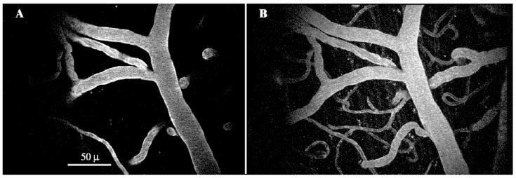
Figure 1.

Blood vessels on the surface of the brain, as viewed before (left) and after (right) injection of FITC-dextran into a mouse tail vein. These images were collected using Kalman averaging (n=2).

Figure 2.

A mouse tail vein was injected with FITC-dextran to produce angiographical images. The incident laser light was tuned to 800 nm, and power exiting the objective lens was 15 mW. A shows excitation from a single focal plane using multiphoton microscopy (Kalman average of 5 images). B shows a maximum intensity projection of unaveraged images collected in XYZ, where the planar (XY) coordinates match those in A and the Z depth totals 80μ, acquired in 2μ steps from 30μ superficial of A to 50μ deep of A. Note how the vessel cross sections seen in A correspond to diving vessels seen in B.

Figure 3.

Examples of Cerebral Angiography using RITC-dextran (A-C) and FITC-dextran (D). A shows a maximum intensity projection of a stack of 10 images spaced 2μ apart. Bar, 20μ. B (Kalman averaging, n=4) and C (Kalman averaging, n=3) show larger fields of view. Bar, 100μ. D shows how a capillary curves and branches (unaveraged). Bar, 25μ.

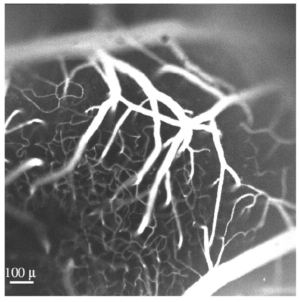
Figure 4.

Mouse brain vasculature as visualized with multi-photon laser-scanning microscopy. This image shows the maximum projection of a z-series of images collected in 5 μ increments between depths of 50-130 μ in the neocortex of an anaesthetized mouse, beneath the middle internal frontal artery. The blood was labeled with dextran-conjugated fluorescein via an injection into the animal’s tail vein, and was viewed through a surgically-prepared “cortical window” (λ_ex = 800 nm, power < 50 mW).

Figure 5.

Motion of blood plasma as measured with two-photon excitation laser scanning microscopy. Yellow-green fluorescent microspheres (Polysciences) of diameter 57nm +/- 8.6 nm were injected into a murine tail vein. The dilution coefficient was previously titrated to optimize for maximal “bead signal” and minimal “bead clumping.” In this case, a 2.5% solution of microspheres was diluted 1:4 in PSB and vortexed just prior to injection. This figure shows microsphere fluorescence passing in one scan (at 133 msec). The field of view lies longitudinally within a large artery. Data were acquired at 15 Hz. The velocity of the bead or small bead clump shown here is 1.266 mm/sec.

2.2. Seeing the Brain Cells

Whereas loading of fluorescent contrast into the brain’s vasculature is fairly simple, the loading of contrast into the brain cells themselves is comparatively challenging (Allport and Weissleder 2001). While preparations of cell cultures and tissue slices have benefited by the use of acetoxymethyl esters (to facilitate the introduction of fluorescent dyes) and biolistic loading with a “gene gun” (to facilitate the introduction of fluorescent protein genes), neither of these vehicles is practical for getting cells to fluoresce in intact, adult animals. Nevertheless, there are at least four possible approaches for labeling cells in vivo. The first of these, extracellular injection of dye, is the most parsimonious but the least effective. While some dye is endocytosed by cells, the labeling pattern is that a few saturated cells are present in a noisy background at the injection site, and autofluorescence is seen elsewhere. Another approach is intracellular injection of dye (Svoboda, Denk et al. 1997). This approach has been successful, although the number of cells that may injected during a single recording session is practically constrained. A third approach is to generate transgenic animals expressing fluorescent proteins (Zhuo, Sun et al. 1997; Nolte, Matyash et al. 2001). While this approach has been successful, it may suffer from unwanted biological effects due to constitutive expression of the transgene throughout development. A fourth approach, demonstrated here, involves the injection of viral vectors that genetically encode for fluorescent proteins (Griesbeck, Yoder et al. 2000). Mice were anesthetized with ketamine-xylazine (50 mg/kg and 15 mg/kg, I.P.) and placed into a stereotactic apparatus. A hole (bur size FG 1/2) was drilled in the skull over sensory cortex. An adenoviral vector for yellow cameleon 2.1 (i.e. genetically encoding for both cyan and yellow fluorescent proteins, under the control of the cytomagaloviral promoter) was loaded into beveled glass electrodes, and pressure injected (20 psi for 100 msec or 1320 nl virus with titer of 20,000 PFU/nl) intracranially at depths of 0.25 mm, 0.5 mm, and 1 mm. Following a minimum in vivo incubation and recovery time of two days, mice were urethane-anesthetized and cortical windows were prepared over sensory cortex. As seen in Figure 6, limited fluorescence is present at the injection site itself. Figures 7 and 8 show the cellular expression pattern of fluorescent proteins as observed in vivo through cortical windows. This “fluorescent loading” method results in the expression of genetically-encoded fluorescence in morphologically distinct cell types in the brain, as seen in Figure 9.

Figure 6.

Injection site of an intracerebral adenoviral pressure injection. The electrode tract is visible in A and B. A shows the brain tissue as immunolabeled with S100β, an astrocyte marker, tagged with CY5. B shows yellow fluorescent protein (YFP) that is expressed in cells infected by an adenoviral vector that encodes for YFP. Each image is kalman-averaged (n=10). Note that the fluorescence pattern of YFP is such that most cells in the immediate vicinity of the injection are not labeled. This is in contrast to the fluorescence pattern of intracerebrally-injected fluorescent dyes.

Figure 7.

Brain cells expressing genetically-encoded fluorescence as viewed in a living mouse. The sensory cortex of an adult mouse was injected with an adenovirus that genetically encodes for both cyan fluorescent protein (CFP) and yellow fluorescent protein (YFP). This image shows the expression of CFP in the mouse’s brain at a time of two days post-injection and a distance of 400 μ from the injection tract. Note the cytoplasmic fluorescence, and the exclusion of nuclear labeling (Kalman=5; λ = 800 nm; power=100 mW).

Figure 8.

Brain cells expressing genetically-encoded fluorescence as viewed in combination with angiography in a living mouse. The sensory cortex of an adult mouse was injected with an adenovirus that genetically encodes for both CFP (left channel) and YFP (right channel). Angiography was performed via an intravenous injection of FITC-dextran (right channel). This image shows a maximum intensity projection for a z-series of 16 μ depth, in 1 μ steps. Imaging was performed 7 days following adenoviral injection and labeled cells are at a distance of 250 μ from the injection site (Kalman=8; λ_ex = 800 nm; power=50 mW).

Figure 9.

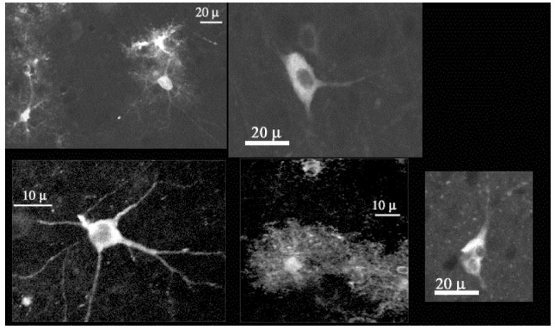
Yellow cameleon 2.1, which genetically encodes for both CFP and YFP, may be loaded into brain cells of intact adult animals via injection of an adenoviral vector that encodes for the proteins. This loading method results in the expression of genetically encoded fluorescence in morphologically distinct cell types – including multipolar, stellate, and multinucleated - in the brain. Examples of such YFP expression are seen here.

2.3. Optical Contrast via Intracerebral Injection of Adenoviral Vectors: Identification of Cells Expressing Fluorescent Proteins

At the end of each imaging session, the mice were transcardially perfused with fixative and their brains were extracted for immunohistochemical processing. Since infected cells were of various morphologies, the injected tissue was immunolabeled in an effort to identify if neurons or astrocytes expressed the genetically encoded fluorescence. Astrocytes were labeled using an antibody specific to either glial fibrillary acidic protein (GFAP) or S100β, and neurons were labeled using an antibody that recognizes neurofilament protein (NF).

YFP was detected in the corpus callosum, ventricles, astrocytes near the cortical surface (glial limitans), cortex, and striatum (Figure 10). Expression in these areas was not always restricted to the local vicinity of the injected area; for example, YFP+ cells near the brain surface were observed as far as 1.8 mm anterior to the injection site; in the corpus callosum, YFP+ cells were observed as far as 1.25 mm posterior to the injection site. Expression of genetically-encoded fluorescence in the striatum and the cerebral cortex was typically restricted to within 225 μ of the injection tract. The majority (73.5%, n=34) of the YFP+ cells near the cortical surface labeled positively with an astrocyte marker, S100β. Examples of such cells are shown in Figure 11. While the remaining fluorescent cells (YFP+/S100β-) in this region were not identified histochemically, some may be leptomeningeal cells. YFP+/S100β+ cells were also observed in the cortex (52%, n= 23), striatum (31%, n=29) and corpus callosum (50%, n=16). Most of the YFP+/S100β- cells in the cortex and striatum were identified as neurons (NF+). The YFP+/S100β- cells in the corpus callosum were not identified histochemically; they appeared to be oligodendrocytes. The fluorescent protein in ventricles did not appear to be positive for S100β and was likely being expressed by ependymal cells. Different viral vectors and promoters may infect different cellular populations (e.g. Chen, Lendvai et al. 2000).

Figure 10.

This montage shows a coronal section of a mouse brain that was injected with an adenoviral vector encoding fluorescent protein. The pink color indicates the location of YFP and the blue indicates S100β labeled with CY5 and serves as a “counterstain.” The expression of genetically encoded fluorescent protein was distributed into four areas: (A) near the surface of the cortex (near and anterior to the injection site), (B) in cortex proximal to the injection tract, (C) in the corpus callosum (near and posterior to the injection site), and (D) in the striatum (near the injection site). Some labeling was seen in the lateral ventricle of the injected hemisphere.

Figure 11.

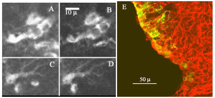
Co-localization of YFP with astrocyte markers. Note the co-localization of YFP (B,D) and S100β, an astrocyte marker (A,C). D shows a merged image, with YFP in green and GFAP in red. Yellow indicates areas of co-localization for YFP and GFAP. All images are kalman-averaged (n=10).

2.4. Immunohistochemical Methods

Brains were fixed with 4% paraformaldehyde and sliced coronally into 25 μ sections. Nonspecific aldehyde sites were blocked with PBS/glycine and sections were incubated in a general blocking buffer (PBS/glycine 3% normal goat serum, 1% BSA). This was diluted 1:3 to obtain a working buffer used throughout the remaining procedure. Overnight incubation in primary antibodies plus Triton X-100 (1%) at 4°C was followed by incubation in goat anti-rabbit Cy5 IgG (H + L, Jackson, 1:75) for 1 hr at room temperature. The following primary antibodies were used: Dako rabbit polyclonal to S100β (1:50), Sigma rabbit polyclonal to NF-200kd (1:100), and Sigma rabbit polyclonal to GFAP (1:100). Sections were washed thoroughly, mounted in antifade media, sealed, and viewed with a confocal microscope. Tissue from cameleon–expressing transgenic mice provided a positive control. Negative controls included uninjected but processed tissue, tissue processed without primary antibody, and unprocessed tissue (to determine autofluorescence at the relevant optical settings).

3. Surgical Preparation of Mice for Brain Imaging

3.1. Surgery Basics

CD-1 NIH Swiss Mice (Charles River) were anesthetized with urethane (1-2 mg/g body weight, administered interperitoneally and as a split dose separated by 10 min) and placed into a small animal stereotaxic apparatus with a mouse adaptor (Kopf 926) and custom-built head supports. Their body temperature was maintained at 36.5°C by a homeothermic blanket system with flexible probe (Harvard Apparatus) that was adapted to fit a murine rectum. Puralube Vet Ointment was applied to the eyes to prevent dryness. Animals breathed oxygen gas saturated with water vapor. Hourly supplements of 0.1 ml physiological ringer (including 10mM glucose) were administered subcutaneously. The skin over the skull was reflected and the imaging region was marked. The skull was dried and the imaging region was prepared by one of the two methods described below.

3.2. Cortical Window Preparation

This method, used previously with rats, was adapted for mice. A 2-3 μ² window of skull was removed over the imaging region with a dental air drill and FG 1/4 bur (Midwest). Bone wax was applied as necessary to control bleeding from the skull’s vasculature. The dura mater – which, at least in this mouse strain, is of negligible thickness – was left intact and did not impede imaging. A stainless steel headframe (Figure 12) – used to stabilize the animal’s head to a holder attached to the optical bench – was cemented to the surrounding skull with dental acrylic (Lang). Moisture of exposed brain regions was maintained by a surgical gelatin sponge (Upjohn) that was saturated with artificial cerebral spinal fluid (ACSF). This sponge was removed just prior to sealing the exposed brain surface to a glass coverslip via an agarose plug (2% in ACSF). The glass coverslip was secured to the headframe. Imaging was performed primarily with water immersion objective lenses that sat (in water) at the surface of the coverslip. This method allows for the maximum focal penetration into neocortex that may presently be attained with optical techniques. It does not suffer from high light scattering by the skull, or unmatched refractive indices between the skull and aqueous solutions (e.g. ACSF, agarose, or ddH₂O). Figure 13 shows a low magnification view of the cerebral vasculature as viewed through a cortical window. A caveat of this method is that the removal of skull renders the brain susceptible to pressure and temperature changes, which hastens the decline of the animals and thus reduces recording time.

Figure 12.

Design of the headframe used to image the brains of intact mice. The center ellipse was placed over the imaging region, and the surrounding recessed area served as either a space to secure a glass coverslip (for the “cortical window” preparation) or as a reservoir of ACSF to keep the skull moist (for the “through skull” preparation).

This figure is used with permission from Wiley-Liss, Inc., a subsidiary of John Wiley & Sons, Inc. It originally appeared in “Cortical Imaging Through the Intact Mouse Skull Using Two-Photon Excitation Laser Scanning Microscopy” Yoder et al, Microscopy Research and Technique, Copyright © 2002.

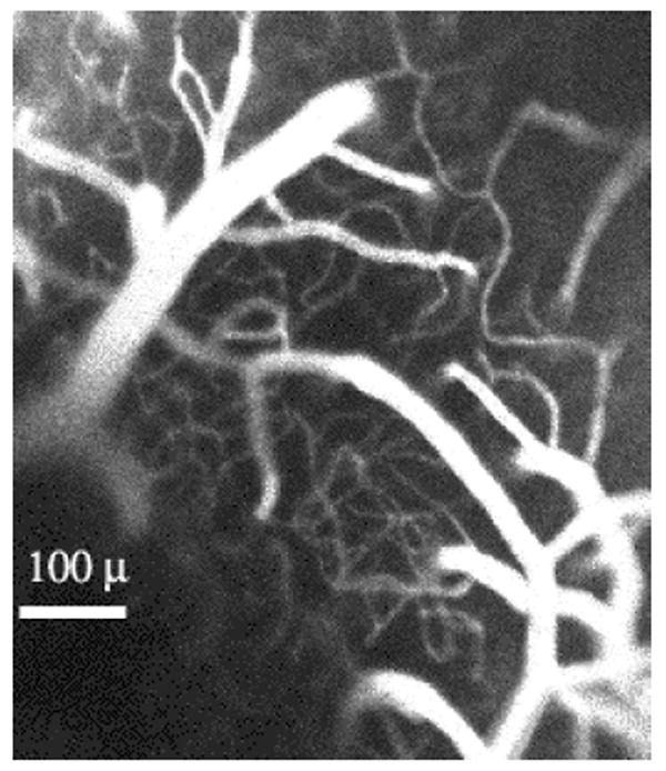
Figure 13.

Cerebral vasculature near the mouse brain surface, labeled with RITC-dextran in the blood serum, and viewed at low magnification through a “cortical window”. Bar, 100 μ.

3.3. Thinned Skull Preparation

In this method, the skull is thinned, but left intact and imaged through (Yoder and Kleinfeld 2002). A 2-3 μ² area of skull over the imaging region was thinned to 200-250 μ with a dental air drill and FG 1/2 bur (Midwest). Superglue (Loctite 493 Instant Adhesive Superbonder 49350) – which scatters light significantly less than bone wax - was used to control bleeding from the skull. No bone wax was applied. A stainless steel headframe (Figure 12) was cemented to the unthinned skull with dental acrylic. This headframe was specifically designed to fit mouse skull; it has the optimal ratio of skull-to-metal needed to secure a firm attachment without having to build up “fake skull” using dental acrylic. It was secured to the imaging apparatus and used to stabilize the animal’s head position during imaging experiments. ACSF was applied over the imaging region and images were obtained using a water immersion objective lens that was placed directly in the ACSF over the skull. While this method adds precision to the image resolution observed during intrinsic optical imaging techniques (Masino, Kwon et al. 1993), it does possess two caveats. First, the focal depth attainable in cortex is reduced by at least the depth of the thinned skull. Second, the light scattering by (Figure 14), and different refractive index of, the skull somewhat compromises the image resolution. An asset of this method is that it avoids susceptibility to pressure and temperature changes, and enables longer recording periods and multiple imaging sessions (Christie, Bacskai et al. 2001).

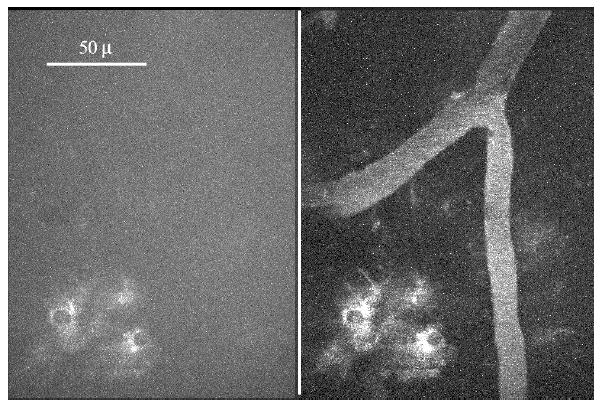
Figure 14.

The skull over mouse somatosensory cortex was thinned, and FITC-dextran was injected into the blood stream. Multiphoton microscopy was used image through the skull and down into the brain (λ_ex = 805 nm). A shows a maximum intensity projection of unaveraged images acquired in skull during XYZ acquisition, where Z = 0 to −90 μ in -3 μ increments (power = 5 mW). The scratchmark was made by the drill while thinning the skull. B shows a maximum intensity projection of unaveraged images acquired along the interface between the curving skull and brain. The depth is −150 to −201 μ, and images were collected in -3 μ increments (power = 10 mW). In this image, a vessel at the brain surface starts to appear; in other fields the vasculature within the skull itself was observed. Note the differences in light scattering between the skull and the brain tissue. No correction was made for the refractive differences between the skull and the brain tissue.

4. In Vivo Imaging: Issues and Problems

4.1. Motion

One of the most common problems encountered during in vivo imaging is motion artifact. Motion effects may be grouped into two categories - external motion, where the brain is moved as a whole, and internal motion, where motion occurs within the brain itself. An obvious strategy for dealing with sources of motion external to the brain is to improve the stability of the interface between the head and the imaging apparatus, thereby removing or reducing the motion artifact during data acquisition. Failing this, corrections for motion during data analysis may be possible. If a fiducial marker was present (be it from autofluorescence or experimentally-introduced contrast), it might provide a means to track a region of interest (ROI) and reregister images. Generally, this requires that the range of motion for the ROI was fully captured within the dimensions (planar and 3D) recorded by the images. Motion internal to the brain is not readily alleviated, as it is often either part of a genuine physiological response or related to the “vasomotion” indicative of a living animal. Nevertheless, the impact of “physiological noise” may be minimized by collecting images at rates distinct from biological rhythms. Futhermore, signal fidelity may be improved by filtering the frequencies associated with respiratory and cardiac cycles.

4.2. Physiological Monitoring

Physiological monitoring of animals serves many purposes. It tracks the animal’s viability, to verify when the animal is healthy and to communicate in real time when it is not. Physiological monitoring can provide control data for systemic responses to experimental stimuli (such as the changes in breathing during hypercapnic stimulation). To the extent that respiration, heart rate, or blood pressure generate “physiological noise”, the imaging SNR may be improved by gating image acquisition to a physiological signal or by using the physiological data to filter the imaging signals during post-processing. Further, as anesthetized animals do not properly thermoregulate, this function may be provided by feedback from a temperature monitoring system.

4.3. Anesthesia

The use of anesthetized animals for in vivo imaging reduces motion artifact and allows for invasive procedures. However, its use introduces some confounding effects that are not fully understood (Lahti, Ferris et al. 1998). Some neuronal activity is resilient during anesthesia, in that electrical responses to stimuli are observed. However, glial activity may be directly antagonized by some anesthetics (Finkbeiner 1992) and anesthetics exert wide-ranging effects on cerebral blood flow (Lindauer, Villringer et al. 1993). These matters should be considered when interpretting data collected on anesthetized animals.

5. Multiphoton Microscopy of the Cerebral Vasculature: Baseline Activity and Response to Hypercapnic Stimulation

5.1. Neurovascular Responses: What are the Parameters?

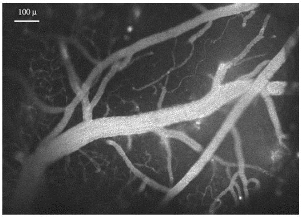
Brain activation is evident in cerebral neurons, glia, and vasculature – although the glial responses have only been recorded in vitro and in situ (Verkhratsky, Orkand et al. 1998). The temporal parameters of neuronal, glial, and cerebrovascular responses are not fully characterized in terms of their durations and latencies, but the peak response times suggest a sequence in which neurons respond first (msec), succeeded by astrocyte responses (1-2 s), and then the hemodynamic response (6 s). Even less is known about the spatial parameters of neuronal, glial, and cerebrovascular responses, or the degree of their overlap. In some cases, neuronal receptive fields have been mapped electrophysiologically and identified as networks of synaptically connected cells. While activity within the astrocyte syncytium has been demonstrated, the glial receptive fields have yet to be identified (Giaume and McCarthy 1996). It has been suggested (Villringer and Dirnagl 1995) that a cerebrovascular receptive field may be defined as the portion of a vascular bed fed by a single penetrating arteriole (Figures 15 and 16), although in practice the dimensions of a cerebrovascular response may depend upon what attribute of the vascular response is recorded (Buxton 2002).

Figure 15.

Top view of penetrating arterioles as they dive into the “spaghetti” of the neocortical capillary bed. The blood was labeled with rhodamine (RITC-dextran) via an injection into the tail vein of an anaesthetized mouse. One current hypothesis is that the size of a “vascular receptive field” is determined by the volume of brain fed by a single penetrating arteriole (see text).

Figure 16.

This image, acquired by confocal laser scanning microscopy (one-photon excitation, λ_ex = 568 nm, Kalman=5) displays the rhodamine-labeled cerebral vasculature in a mouse’s primary sensory cortex. Note the penetrating arterioles as they give rise to the capillary plexus, or “spaghetti”. The capillary bed contains many loops, a characteristic that is consistent with the substantial variability in the baseline flow.

5.2. Variability of Baseline Capillary Blood Flow

When attempting to determine the parameters of a cerebrovascular response, the question of resolution arises. Nonoptical neuroimaging techniques tend toward a “top down” approach, by measuring macrovascular-dominated signals over large areas of brain. Optical techniques have the spatial resolution to afford a “bottom up” approach. The first step is to consider if individual capillaries, the smallest vessels of the microvasculature, are reliably responsive. The cerebral capillary bed is a tortuous structure, marked by bifurcations and loops, as evidenced in its “spaghetti” appearance (Figures 15, 16, 17). This geometry suggests that the net direction of flow within a capillary segment need not be determined, as it is along arterial and venous routes. In order to directly examine flow in single capillary segments, Villringer and coworkers (1994) developed a technique that combined angiography with confocal laser scanning microscopy to watch the motion of blood cells within a capillary. Angiography brightly labels the blood plasma but not the blood cells. Thus, when a vessel’s diameter approaches the size of a blood cell – as is the case with capillaries – the blood cells themselves may be visualized as nonfluorescent “dark regions” and their motion may be recorded (Villringer, Them et al. 1994). This technique was adapted for multiphoton microscopy (Kleinfeld, Mitra et al. 1998). Indeed, the basal motion of blood cells through capillaries exhibits significant variability. Examples of this “biological noise” within the capillary bed include stalls of the blood cells and reversals of their flow direction (Figures 18 and 19) and the frequent of occurrence of microstrokes (Figures 20 and 21). Interestingly, while the basal flow is characterized by fluctuations in healthy tissue, it is possible that the variability may be reduced under pathological conditions (Figure 22).

Figure 17.

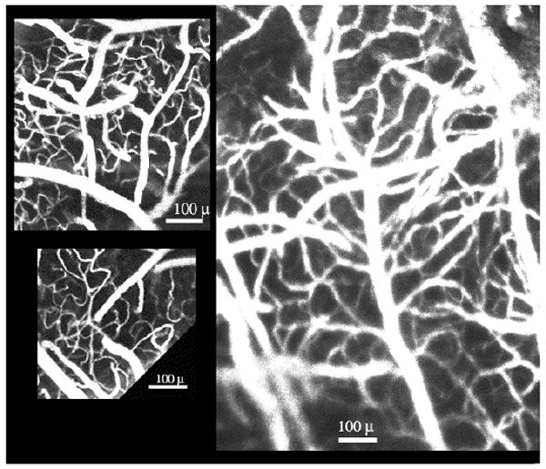
Scenes from within the “spaghetti”. Note the pronounced tortuosity of the capillaries. Images on the left are from a mouse injected intravenously with FITC-dextran (Kalman averaging, n=5). The image on the right is from a mouse injected intravenously with RITC-dextran (Kalman averaging, n=4). Bar, 100 μ.

Figure 18.

This field, as viewed by multiphoton microscopy (λ_ex = 790 nm), shows a putative arteriole as it gives rise to a curving capillary. The blood stream was labeled with RITC-dextran, and the image was Kalman averaged (n=5). A segment of this capillary was monitored in time series (see Figure 19).

Figure 19.

These images show a capillary segment from the field depicted in Figure 18. These images were collected in sequence during time series acquired at 4 Hz. Note that the blood cells (appearing as dark bands) initially flow to the left (A, B, C), then reverse their direction (D, E) to the right (F). Time series may be viewed as Quicktime movies at http://fmri.ucsd.edu/~yoder/.

Figure 20.

This field of view is 300 μ deep in the primary somatosensory cortex of an anesthetized mouse whose blood stream was injected with dextran-conjugated Texas Red. This Kalman-averaged image was collected via multiphoton microscopy (λ_ex = 800 nm). This field is within the “spaghetti” of the capillary bed. Note the cross-sectional appearance of a diving arteriole or venule (*) and several bifurcations of capillaries. One t-junction (arrow) was studied in time series (see Figure 21).

Figure 21.

Images were acquired by two-photon laser scanning microscopy at 6 Hz. A capillary t-junction (indicated in Figure 20) was monitored over time; blood cells appear as dark objects against a bright background of blood plasma. This montage documents the occurrence of a microstroke, whereby the blood flow in the left branch of the t-junction is transiently obstructed. The timing of the images shown was: A – 0.0 s, B - 72.7 s, C - 78.0 s, D - 81.7 s, E - 84.7 s, F - 84.9 s, G - 85.0 s, H - 85.2 s, I - 89.3 s, J - 91.0 s, K - 91.2 s, L - 91.3 s, M - 91.5 s, N - 91.7 s, and O - 99.2 s. Time series may be viewed in Quicktime format at http://fmri.ucsd.edu/~yoder/.

Figure 22.

A murine tail vein was injected with FITC-dextran, and two-photon microscopy was performed through a cortical window prepared over primary sensory cortex (λ_ex = 800 nm). Two adjacent capillary segments are shown at high (A, field of view 42.4 μ²) and low (B, field of view 200.5 μ²) magnification. Laser power was increased focally at a vascular branch point in a plane 60 μ superficial to these segments. This created a lesion that directly affected flow in the capillary on the left, where permanent stagnation of blood cells (elliptical dark objects) was observed. Interestingly, the permanent occlusion of blood cell flux in the left capillary was concomitant with unusual flow parameters in the right capillary. Throughout a time span of over 2 hrs, the right capillary did not exhibit the typical variations in baseline blood cell flux, and the flux was higher than usual, nearing the rates seen under hypercapnic conditions (Figure 24). These data suggest that undamaged capillaries might experience a compensatory increase of baseline blood cell flux when adjacent to vascular lesions.

5.3. Setting the Scale for Blood Flow Changes: Direct Vascular Stimulation

Single-trial responses of capillaries following sensory stimulation are either not detected or are modest, perhaps due to the high baseline variability of the flow (Kleinfeld, Mitra et al. 1998). In an effort to step back and establish the scale for vascular changes, the vasculature was stimulated directly by inducing a hypercapnic state in the animal. This state was induced by replacing the O₂ gas normally inhaled with CO₂ (10% as regulated by a Matheson flowmeter). Identification of surface arteries and veins was confirmed with the use of dichroics: 470DF15 was used to view veins and 560DF10 was used to view arteries, in accordance with the published absorption spectra for hemoglobin and deoxyhemoglobin (Lemberg and Legge 1949). Respiration signals were amplified and filtered before being acquired by Labview at 200 Hz; these signals verified the delivery of CO₂. Vessels were viewed through thinned skull using angiography. While venous changes were not readily apparent, consistent and significant changes in arteries (Figure 23) and capillaries (Figure 24 and 25) were observed.

Figure 23.

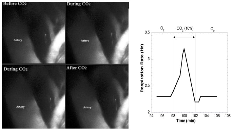
Arterial Response to Hypercapnic Stimulation. A branch of the middle cerebral artery is shown before, during, and after CO₂ inhalation. During hypercapnia, the artery dilated (18-25% increase in vessel caliber), an effect that was reversed upon return to O₂. A concomitant change in respiration rate during CO₂ inhalation was recorded. Each image is a maximal intensity projection of planar scans spaced 3μ apart. The field of view is 160μ². The depth is 246-303μ, just below the skull. Acquisition time for each stack was 90s (FITC-dextran, Kalman=3, λ_ex = 800 nm, 40 mW).

Figure 24.

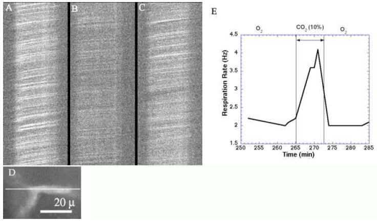
Capillary Response to Hypercapnic Stimulation. The image of a capillary (D) was rotated so that the capillary’s longitudinal orientation was positioned along the X-scan direction, as indicated. XT scans collected at 490 Hz show the movement of blood cells (dark streaks) before (A), during (B), and after (C) CO₂ inhalation. Note the change in slope (indicative of blood cell velocity and flux) and intensity (indicative of blood cell density) during hypercapnia, and the partial recovery thereafter. Concomitant changes is respiration were recorded (E). Total depth is 400 μ (250 μ in skull, 150 μ in cortex). Images are unaveraged (FITC-dextran, λ_ex = 800 nm, 105 mW).

Figure 25.

These planar images were collected as a stack, spaced 2 μ apart in the zed (Z) direction, and verify that the imaging plane is perpendicular to the capillary on the left. The capillary’s diameter – as seen here in cross section – was examined for baseline fluctuations and responsiveness to hypercapnic stimulation. Diameter changes of 6% were observed with 10% CO₂ (FITC-dextran, λ_ex = 800 nm).

References

- Allport JR, Weissleder R. In vivo imaging of gene and cell therapies. Exp Hematol. 2001;29(11):1237–46. doi: 10.1016/s0301-472x(01)00739-1. [DOI] [PubMed] [Google Scholar]
- Balaban RS, Hampshire VA. Challenges in small animal noninvasive imaging. Ilar J. 2001;42(3):248–62. doi: 10.1093/ilar.42.3.248. [DOI] [PubMed] [Google Scholar]
- Brafield AE, Llewellyn MJ. Animal Energetics. Glasgow, Scotland: Blackie; 1982. [Google Scholar]
- Buxton RB. Introduction to Functional Magnetic Resonance Imaging: Principles and Techniques. New York, NY: Cambridge University Press; 2002. [Google Scholar]
- Chen BE, Lendvai B, et al. Imaging high-resolution structure of GFP-expressing neurons in neocortex in vivo. Learn Mem. 2000;7(6):433–41. doi: 10.1101/lm.32700. [DOI] [PubMed] [Google Scholar]
- Christie RH, Bacskai BJ, et al. Growth arrest of individual senile plaques in a model of Alzheimer’s disease observed by in vivo multiphoton microscopy. J Neurosci. 2001;21(3):858–64. doi: 10.1523/JNEUROSCI.21-03-00858.2001. [DOI] [PMC free article] [PubMed] [Google Scholar]
- Denk W, Svoboda K. Photon upmanship: why multiphoton imaging is more than a gimmick. Neuron. 1997;18(3):351–7. doi: 10.1016/s0896-6273(00)81237-4. [DOI] [PubMed] [Google Scholar]
- Finkbeiner S. Calcium waves in astrocytes-filling in the gaps. Neuron. 1992;8(6):1101–8. doi: 10.1016/0896-6273(92)90131-v. [DOI] [PubMed] [Google Scholar]
- Giaume C, McCarthy KD. Control of gap-junctional communication in astrocytic networks. Trends Neurosci. 1996;19(8):319–25. doi: 10.1016/0166-2236(96)10046-1. [DOI] [PubMed] [Google Scholar]
- Griesbeck O, Yoder EJ, et al. In Vivo Expression of Cameleons in Rodent Neocortex by Adenoviral Gene Transfer. Society for Neuroscience Abstracts. 2000;26:874. [Google Scholar]
- Hecht J. The Laser Guidebook. New York, NY: McGraw-Hill; 1992. [Google Scholar]
- Kleinfeld D, Mitra PP, et al. Fluctuations and stimulus-induced changes in blood flow observed in individual capillaries in layers 2 through 4 of rat neocortex. Proc Natl Acad Sci U S A. 1998;95(26):15741–6. doi: 10.1073/pnas.95.26.15741. [DOI] [PMC free article] [PubMed] [Google Scholar]
- Lahti KM, Ferris CF, et al. Imaging brain activity in conscious animals using functional MRI. J Neurosci Methods. 1998;82(1):75–83. doi: 10.1016/s0165-0270(98)00037-5. [DOI] [PubMed] [Google Scholar]
- Lemberg R, Legge JW. Hematin Compounds and Bile Pigments; their constitution, metabolism, and function. New York: Interscience Publishers; 1949. [Google Scholar]
- Lindauer U, Villringer A, et al. Characterization of CBF response to somatosensory stimulation: model and influence of anesthetics. Am J Physiol. 1993;264(4 Pt 2):H1223–8. doi: 10.1152/ajpheart.1993.264.4.H1223. [DOI] [PubMed] [Google Scholar]
- Masino SA, Kwon MC, et al. Characterization of functional organization within rat barrel cortex using intrinsic signal optical imaging through a thinned skull. Proc Natl Acad Sci U S A. 1993;90(21):9998–10002. doi: 10.1073/pnas.90.21.9998. [DOI] [PMC free article] [PubMed] [Google Scholar]
- Nolte C, Matyash M, et al. GFAP promoter-controlled EGFP-expressing transgenic mice: a tool to visualize astrocytes and astrogliosis in living brain tissue. Glia. 2001;33(1):72–86. [PubMed] [Google Scholar]
- Oheim M, Beaurepaire E, et al. Two-photon microscopy in brain tissue: parameters influencing the imaging depth. J Neurosci Methods. 2001;111(1):29–37. doi: 10.1016/s0165-0270(01)00438-1. [DOI] [PubMed] [Google Scholar]
- Svoboda K, Denk W, et al. In vivo dendritic calcium dynamics in neocortical pyramidal neurons. Nature. 1997;385(6612):161–5. doi: 10.1038/385161a0. [DOI] [PubMed] [Google Scholar]
- Tsai PS, Nishimura N, Yoder EJ, et al. Principles, design, and construction of a two photon laser scanning microscope for in vitro and in vivo brain imaging. In: Frostig R, editor. Methods for In Vivo Optical Imaging. Boca Raton. FL: CRC Press; 2002. [Google Scholar]
- Verkhratsky A, Orkand RK, et al. Glial calcium: homeostasis and signaling function. Physiol Rev. 1998;78(1):99–141. doi: 10.1152/physrev.1998.78.1.99. [DOI] [PubMed] [Google Scholar]
- Villringer A, Dirnagl U. Coupling of brain activity and cerebral blood flow: basis of functional neuroimaging. Cerebrovasc Brain Metab Rev. 1995;7(3):240–76. [PubMed] [Google Scholar]
- Villringer A, Dirnagl U, editors. Optical Imaging of Brain Function and Metabolism II. New York, NY: Plenum Press; 1997. [Google Scholar]
- Villringer A, Them A, et al. Capillary perfusion of the rat brain cortex. An in vivo confocal microscopy study. Circ Res. 1994;75(1):55–62. doi: 10.1161/01.res.75.1.55. [DOI] [PubMed] [Google Scholar]
- Yoder EJ, Kleinfeld D. Cortical imaging through the intact mouse skull using two-photon excitation laser scanning microscopy. Microsc Res Tech. 2002;56(4):304–5. doi: 10.1002/jemt.10002. [DOI] [PubMed] [Google Scholar]
- Zhuo L, Sun B, et al. Live astrocytes visualized by green fluorescent protein in transgenic mice. Dev Biol. 1997;187(1):36–42. doi: 10.1006/dbio.1997.8601. [DOI] [PubMed] [Google Scholar]