Unbiased Average Age-Appropriate Atlases for Pediatric Studies

Abstract

Spatial normalization, registration, and segmentation techniques for Magnetic Resonance Imaging (MRI) often use a target or template volume to facilitate processing, take advantage of prior information, and define a common coordinate system for analysis. In the neuroimaging literature, the MNI305 Talairach-like coordinate system is often used as a standard template. However, when studying pediatric populations, variation from the adult brain makes the MNI305 suboptimal for processing brain images of children. Morphological changes occurring during development render the use of age-appropriate templates desirable to reduce potential errors and minimize bias during processing of pediatric data. This paper presents the methods used to create unbiased, age-appropriate MRI atlas templates for pediatric studies that represent the average anatomy for the age range of 4.5–18.5 years, while maintaining a high level of anatomical detail and contrast. The creation of anatomical T1-weighted, T2-weighted, and proton density-weighted templates for specific developmentally important age-ranges, used data derived from the largest epidemiological, representative (healthy and normal) sample of the U.S. population, where each subject was carefully screened for medical and psychiatric factors and characterized using established neuropsychological and behavioral assessments. . Use of these age-specific templates was evaluated by computing average tissue maps for gray matter, white matter, and cerebrospinal fluid for each specific age range, and by conducting an exemplar voxel-wise deformation-based morphometry study using 66 young (4.5–6.9 years) participants to demonstrate the benefits of using the age-appropriate templates. The public availability of these atlases/templates will facilitate analysis of pediatric MRI data and enable comparison of results between studies in a common standardized space specific to pediatric research.

Introduction

Magnetic resonance imaging (MRI) has emerged as the premier modality of noninvasive imaging of normal structural and metabolic development of the brain in both infants and children. With the advent of modern MRI methods in the last 20 years, multiple groups have reported age-related changes in gray matter (GM) and white matter (WM) volumes, extent of myelination, and subcortical structures (Jernigan and Tallal 1990; Jernigan, Trauner et al. 1991; Filipek, Richelme et al. 1994; Pfefferbaum, Mathalon et al. 1994; Blatter, Bigler et al. 1995; Caviness, Kennedy et al. 1996; Giedd, Rumsey et al. 1996; Giedd, Vaituzis et al. 1996; Reiss, Abrams et al. 1996; Lange, Giedd et al. 1997; Kennedy, Lange et al. 1998; Caviness, Lange et al. 1999; Giedd, Blumenthal et al. 1999; Paus, Zijdenbos et al. 1999; Sowell, Thompson et al. 1999; Courchesne, Chisum et al. 2000; Bartzokis, Beckson et al. 2001; Blanton, Levitt et al. 2001; De Bellis, Keshavan et al. 2001; Durston, Hulshoff Pol et al. 2001; Mazziotta, Toga et al. 2001; Gogtay, Giedd et al. 2002; Sowell, Thompson et al. 2002; Kennedy, Haselgrove et al. 2003; Sowell, Peterson et al. 2003; Blanton, Levitt et al. 2004; Gogtay, Giedd et al. 2004; Sowell, Thompson et al. 2004; Sowell, Thompson et al. 2004). However, significant variability has generally been seen in the volumetric and metabolic data across populations and between genders, complicated by reports of differences in regionally specific changes within individual brain growth trajectories (Giedd, Rumsey et al. 1996; Giedd, Blumenthal et al. 1999; Gogtay, Giedd et al. 2004). Furthermore, because most prior studies have limited number of subjects and included analysis of T1-weighted (T1w) data only, previous findings have not been easily extrapolated among studies, between specific age-groups, or to the general pediatric population.

To address these issues, the National Institutes of Health (NIH) MRI Study of Normal Brain Development has developed a large, combined cross-sectional and longitudinal, population-based study design to generate a meaningful normative database of T1-weighted (T1w), T2w and proton density weighted (PDw) structural images that will be useful in the study of both normal brain development, and childhood neurological and neuropsychiatric diseases (Evans 2006; Almli, Rivkin et al. 2007). Previous reports (Evans and Group 2006), (Almli, Rivkin et al. 2007), (Waber, De Moor et al. 2007) have detailed the study‘s design, imaging protocols and analysis, and behavioral/cognitive testing methods. This report describes the creation and usefulness of age-appropriate atlases based on the Objective 1 data (i.e., subjects aged 4.5–18.5 years) from the MRI Study of Normal Brain Development.

In addition, data characterizing cognitive and behavioral constructs for all infants, children, and adolescents in the study were acquired along with structural imaging data to enable examination and characterization of correlations between structure and function associated with ongoing developmental processes. Our hope is that the construction of a population-based, representative database of MRI structural and metabolic data correlated with validated cognitive/behavioral measurements will improve our ability to detect and interpret differences in brain development that correspond to pediatric psychiatric and neurological disorders.

Many automated techniques for registration, tissue classification, and statistical analysis use a template brain (Mazziotta, Toga et al. 2001), including mni_autoreg (Collins, Neelin et al. 1994), SPM (Ashburner and Friston 1997), and FSL (Smith, Jenkinson et al. 2004). However, such techniques are not ideal for pediatric analysis because the templates were created by averaging MRI data from young adults. Since the developing brain is not simply a smaller version of an adult brain, the use of adult templates may introduce a bias in analysis. For example, (Muzik, Chugani et al. 2000) showed that, when using an adult template with SPM96, the registration of pediatric data was more variable than that of adult data. In addition, Wilke et al. (Wilke, Schmithorst et al. 2002) found that the analysis of pediatric data depended greatly on processing techniques and spatial normalization methods. In electroencephalography source analysis, Hoeksma et al. (Hoeksma, Kenemans et al. 2005) found differences between pediatric and adult data, and demonstrated that an adult target was less adequate for pediatric data. Machilsen et al. (Machilsen, d'Agostino et al. 2007) also found standard registration methods using the MNI (Montreal Neurological Institute) template to be less robust with pediatric data.

These types of problems indicate a need for developmental age specific brain templates. To achieve this age specificity, some studies have used data from a single subject for the template. For example, Jelacic et al. (Jelacic, de Regt et al. 2006) built an interactive Web-based atlas for subjects under 4 years of age that facilitates the comparison of a given subject with standard datasets from a database. Shan et al. (Shan, Parra et al. 2006) built a digital pediatric brain structure atlas from T1w MRI scans from a single 9-year-old subject. However, the main problem with using single subject templates is that, despite being a typical healthy individual, the chosen subject may represent an extreme tail of the normal distribution for some brain regions. Moreover, a single subject template cannot represent the anatomical variability in the population. The solution to these problems is to build atlases from multiple subjects. In the pediatric literature, Joshi et al. (Joshi, Davis et al. 2004) used unbiased diffeomorphic atlas construction techniques to build a template of eight 2-year-old subjects. Kazemi et al. (Kazemi, Moghaddam et al. 2007) developed a neonatal atlas for spatial normalization of whole brain MRI, based on data from seven subjects. Bhatia et al. (Bhatia, Aljabar et al. 2007) used an expectation-maximization framework to build an MRI atlas for 1- and 2-year-olds. However, these atlases either were created from a small number of subjects or cover a very narrow age range. More recently, Wilke et al. (Wilke, Holland et al. 2008) created a “Template-O-Matic” toolbox for creating population-specific templates based on the unsupervised tissue segmentation and linear coregistration of individual pediatric scans with regression on independent variables such as age and gender. Although this enables a user to generate an appropriate intensity average template volume for a particular study, anatomical details may be blurred in regions of high variability such as the cortex because only linear registration is used. Therefore, in this paper we create a series of age-specific, nonlinearly registered pediatric templates from 324 subjects within the age range of 4.5 to 18.5 years that include T1w, T2w, and PDw averages as well as average tissue maps for GM, WM, and cerebrospinal fluid (CSF). Because the atlas-building process uses nonlinear registration, these templates have the advantage of being age-specific while retaining significant anatomical detail.

Many groups have investigated techniques for creating an anatomical average from a group of subjects such that the result is representative of the population. In some of the first work published on this topic, Guimond et al. (1998; 2000) developed methods of building a template atlas with both average intensity and average shape. These methods begin by selecting or creating an initial template, which may be a single subject or a linear average like the MNI305 volume used in mni_autoreg, SPM, or FSL. Each subject in the group is then nonlinearly registered to the template, and the estimated transformation is used to resample the subject‘s MRI in the template space. A voxel-by-voxel average is computed across all subjects to produce the average-intensity image, and to warp this image to have an average shape, all nonlinear transformations are averaged together. The inverse of the average nonlinear transformation is then applied to resample the average-intensity image, resulting in a template with both an average unbiased shape and average intensity. To account for imperfections in the nonlinear registration procedure, multiple iterations are performed, each time using the new template as the registration target, until the difference between two successive templates is smaller than some threshold.

This procedure has been used as a general strategy in many subsequent papers that addressed different issues in the template-building process, such as the selection of the first template, data used to build the template, similarity function used to drive the registration, type of nonlinear transformation modeled, and method used for averaging. For example, Stattuck et al. (Shattuck, Mirza et al. 2008) used the nonlinear registration methods of AIR (Woods, Grafton et al. 1998), FSL (Smith, Jenkinson et al. 2004), and SPM to create average targets from 40 healthy normal controls. Wang et al. (Wang, Seghers et al. 2005) evaluated different template construction strategies for atlas-based segmentation and found that an intensity-average template based on nonlinear coregistration was best for the segmentation of 49 brain regions. Joshi and Miller (2000) and Joshi et al. (Joshi and Miller 2000; Joshi, Davis et al. 2004) used diffeomorphic registration to build unbiased average templates, a technique later modified by Lorenzen et al. (Lorenzen, Davis et al. 2005) to create an unbiased atlas as a Fréchet mean estimation process. Bhatia et al. (Bhatia, Aljabar et al. 2007) interleaved tissue classification and nonlinear registration of the tissue probability maps to build an average three-dimensional (3D) MRI template.

To facilitate the processing of pediatric imaging data, we have produced a number of age-appropriate, representative, average brain templates using nonlinear deformation to standard coordinates. The construction of a registration target that is both age-appropriate and representative will allow meaningful correlation of anatomical changes and development. Furthermore, nonlinear deformation methods were used for their superior spatial detail and ability to register anatomies from different subjects and across different ages.

Here, we present the procedure used to create unbiased atlas templates that include a series of symmetric and asymmetric atlases. We created and compared atlases from two databases of MR images covering the age range of 4.5 to 43.5 years: (1) a collection of 324 pediatric (4.5–18.5 years) MRI scans from the NIH-funded MRI Study of Normal Brain Development (hereafter, NIHPD, for NIH pediatric database) (Evans 2006) and (2) an MRI database of young adult brains, using data from 152 subjects (aged 18–43.5 years) acquired at the Montreal Neurological Institute (MNI) as part of the International Consortium for Brain Mapping (known as the ICBM database) (Mazziotta, Toga et al. 1995). These data were used to create templates with the following characteristics: (1) average (over the population analyzed) normalized intensity; (2) average shape; (3) (optionally) left–right symmetry; (4) high contrast-to-noise ratio; (5) high level of anatomical structural detail (as seen in the individual images); and (6) compatibility with new ICBM152 space that is compatible with the older MNI305 stereotaxic space (Janke, Evans et al. 2006).

The main contributions of this paper concern the templates that are created and made available to the scientific community. To our knowledge, this is the only dataset containing (1) an epidemiologically ascertained sample of children aged 4.5 to 18.5 years old, representative of the U.S. population with respect to income (as a proxy for socioeconomic status) and race/ethnicity, (2) where each child has been carefully-screened with respect to medical and psychiatric factors (including family history), and (3) has been very well characterized using a variety of standardized interviews, rating scales and cognitive tests (Evans 2006). These factors ensure that the templates will be useful as normative models.

In addition to the T1w templates for the NIHPD and the ICBM database, the following templates were also created: T2w and PDw templates, average brain masks and probabilistic atlases of GM, WM, and CSF maps. Finally, to demonstrate the usefulness of the pediatric templates, the bias of using a population-specific template is shown by comparing the results obtained using the NIHPD-4.5–18.5 templates and the new ICBM152 template using deformation-based morphometry analysis (Chung, Worsley et al. 2001).

Materials and methods

Creation of an unbiased template

Over the last several years, several competing techniques have been developed for building population-specific templates. The rationale behind building a population-specific atlas is described in (Mazziotta, Toga et al. 2001)); the practical impact of such an atlas on the analysis of functional data is described in Good et al. (Good, Johnsrude et al. 2001), and its impact on the analysis of pediatric data is given in (Wilke M. 2002), (Wilke M. 2003), and (Kazemi, Moghaddam et al. 2007). To reiterate the most important issues, an unbiased brain template is needed (1) to provide a registration target for automatic image processing techniques (e.g., those in (Evans, Collins et al. 1993), (Collins, Neelin et al. 1994), and (Thompson and Toga 2002)); (2) to act as an atlas for volume estimation of brain regions (Amit, Grenander et al. 1991); (Christensen, Rabbitt et al. 1994); (Collins, Zijdenbos et al. 1999); (Mazziotta, Toga et al. 2001); (Mazziotta, Toga et al. 2001); (Toga and Thompson 2001); (Thompson and Toga 2002); (Essen and C. 2002) (Thompson and Toga 2002; Toga and Thompson 2007); (Essen and David 2005); (Seghers, D‘Agostino et al. 2004); (Grabner, Janke et al. 2006)); and (3) to function as a reference for a particular population group in order to study intra- and inter-group variability or growth (Thompson and Toga 2002; Gerig, Davis et al. 2006).

Recently, a number of algorithms have been published for constructing population-specific templates. The first approaches to building average templates were based on manual linear coregistration of individual scans into some kind of normalized reference space (e.g., (Evans, Collins et al. 1993), a process later improved by using automatic tools (Collins, Neelin et al. 1994) to register individual scans into the common space (Janke, Evans et al. 2006). Unfortunately, the variability of human brain anatomy leads to a limited resemblance between the average template and the real scans of individual subjects. Moreover, templates produced by linear registration were not very suitable for the automatic segmentation of brain substructures by deformable template algorithms (Carmichael, Aizenstein et al. 2005). As described above, several methods were developed to produce a template more representative of the anatomy (Guimond, Meunier et al. 1998); (Guimond, Meunier et al. 2000); (Guimond, Roche et al. 2001); (Mazziotta, Toga et al. 2001); (Bhatia, Hajnal et al. 2004); (Joshi, Davis et al. 2004); (Lorenzen, Davis et al. 2005), (Mazziotta, Toga et al. 2001); (Essen and C. 2002); (Wang, Seghers et al. 2005). Generally, these methods may be classified into two types: (1) feature-matching algorithms that rely on matching homologous features of the individual scans and (2) intensity-matching algorithms that use some generic cost function. The procedure described here belongs to the second type.

All templates described below use the original ICBM152 (linear average) template as the initial reference target template volume for linear registration and intensity normalization. Our method is iterative, requiring N (2*N for the symmetric template) nonlinear registrations to be performed at each iteration step, where N is the number of subjects. We empirically show that the method converges to a stable solution after 20 iterations, thus requiring a total of 20*N nonlinear registrations to be performed (40*N for the symmetric template).

Nonlinear average

The work described here depends on the nonlinear registration engine of Automatic Nonlinear Image Matching and Anatomical Labeling (ANIMAL) (Collins et al., 1995). While other non-linear registration techniques could have been chosen (Ardekani, Guckemus et al. 2005), (Avants, Grossman et al. 2006), (Lorenzen and Joshi 2003), , we selected ANIMAL because we have extensive experience with the procedure and a recent study (Guizzard, Fonov et al. 2009) has shown that when used with appropriate parameters, the results of the ANIMAL inter-subject registration procedure are comparable to ART (Ardekani, Guckemus et al. 2005) and SyN (Avants, Epstein et al. 2008), the two top ranked registration procedures in the recent nonlinear registration evaluation paper of Klein et al (Klein, Andersson et al. 2009). While in theory the linear elastic regularization used in ANIMAL does not guarantee the recovered transformation to be diffeomorphic, the set of registration parameters used here constrains the transformation to be smooth, bijective and invertible; characteristics needed for the atlas building procedure described below.

To estimate the required nonlinear transformation between a source and a target volume, the ANIMAL algorithm attempts to match hierarchically image gray-level intensity features in local neighborhoods arranged on a 3D grid by maximizing the cross-correlation of intensities between the source and target images. First, the deformations required to match blurred versions of the source and target data are estimated, producing a dense 3D deformation field, where a displacement vector is stored at each node of the field that best matches the local neighborhoods. Then, this deformation field is upsampled and used as input to the next iteration of the procedure, where the blurring is reduced and the estimation of the deformation field is refined. In this manner, large smooth deformations are recovered first, and finer, more local, deformations are recovered last. The schedule of grid step size, blurring, neighborhood size, and iterations is given in Table 1.

Table 1.

Nonlinear registration parameters. Step size is defined as the distance between control nodes for the free-form deformation recovered by ANIMAL. The blurring kernel is the size of the full-width-half-maximum of the Gaussian kernel used to blur the source and target data. The neighbourhood size is the diameter of the local neighbourhood used to estimate the local correlation that defined local similarity

Iteration	Step size (mm)	Blurring kernel (mm)	Neighborhood size (mm)	Local iterations
1–4	32	16	96	20
5–8	16	8	48	20
9–12	8	4	24	20
13–16	4	2	12	10
17–20	2	1	6	10

Our atlas generation technique is based on the work of (Guimond, Meunier et al. 1998) and (Guimond, Roche et al. 2001) and employs the principles of average model construction using elastic body deformations from (Miller, Banerjee et al. 1997). We use the minimum deformation template notation from the latter. Essentially, the problem can be formulated as follows: Given a set of n 3D MRI volumes (I₁ … I_n), our objective is to find a 3D template Φ, which satisfies two constraints simultaneously, one for intensity, and one for the transformation. The first constraint is to minimize the mean squared intensity difference between the template Φ and each subject I_i, transformed to match the template:

$${\mathrm{\Phi }}^{*}=\text{arg}\underset{\mathrm{\Phi }}{\text{min}}\left[{\displaystyle \sum _{i=1}^n{\displaystyle \underset{\mathit{\text{volume}}}{\mathrm{\int }}{\left(\mathrm{\Phi }(v)-I_i({\mathrm{\Psi }}_{i,\mathrm{\Phi }}(v))\right)}^2\mathit{\text{dv}}}}\right],$$ (1)

where v is a volume coordinate, Ψ_i,Φ are the individual 3D mappings from the template Φ to each subject volume I_i, Φ(v) is the template intensity at location v, and I_i(Ψ_i,Φ(v)) is the intensity in the subject‘s MRI after transformation by Ψ_i,Φ,. The transformation Ψ is constrained using simple elastic body model, such that for each subject i:

$${\mathrm{\Psi }}_{i,\mathrm{\Phi }}=\text{arg}\underset{\mathrm{\Psi }}{\text{min}}{\displaystyle \underset{\mathit{\text{volume}}}{\mathrm{\int }}{\left(\mathrm{\Phi }(v)-I_i(\mathrm{\Psi }(v))\right)}^2\mathit{\text{dv}}}$$ (2)

The second constraint is to minimize the magnitude of all deformations Ψ_i,Φ required to map the template Φ to each subject i:

$${\mathrm{\Phi }}^{*}=\text{arg}\underset{\mathrm{\Phi }}{\text{min}}\left[{\displaystyle \sum _{i=1}^n{\displaystyle \underset{\mathit{\text{volume}}}{\mathrm{\int }}{\left|{\mathrm{\Psi }}_{i,\mathrm{\Phi }}(v)-v\right|}^2\mathit{\text{dv}}}}\right],$$ (3)

In short, we are simultaneously minimizing eq. 1 and 3; equation 2 is minimized for each subject-template pair.

The transformation Ψ_i,T is represented with a dense deformation vector field h, such that Ψ(x) = x + h(x) and Ψ⁻¹(x) = x + h⁻¹(x) where h(x) may be defined on a discrete grid with a given distance (step size) between nodes, as in the ANIMAL algorithm (see Fig. 1). Following this formalism, we have developed an iterative algorithm minimizing the mean square differences in equations 1 and 3. Each iteration of the algorithm interleaves minimization of both objective functions, first the mean square difference in terms of deformations (eq. 3) and second, the mean square difference in terms of intensity (eq. 1). To denote the mapping of each subject found at each consecutive step of the algorithm we use X_i,k, and the current approximation of the template T_k. when the algorithm converges X_i,k → Ψ_i,Φ,,T_k→Φ^* producing the minimum deformation template Φ^* and mapping Ψ_i,Φ., from template to each subject. The algorithm is as follows:

1. Given T_k (the approximation template Φ^* at iteration k), for each scan I_i, calculate X_i,k (mappings from template to an individual scan i, on the iteration k), using the Y¹_i,k−1 (inverse corrected mappings of the scan i, iteration k−1) as a starting point. The identity transform for the first iteration and the linear ICBM152 average was used as T₀.

2. Calculate the residual error based on the average deformation X_0,k of the current template T_k:

   $$X_{0,k}=x+{\displaystyle \sum _n{h}_i(x)/n}$$ (4)

3. Calculate corrected inverse mappings: $Y_{i,k}=X_{i,k}^{-1}•X_{0,k}$, where ‘•’ indicates composition of transformations. This step corresponds to the function minimization of eq. 3 (i.e, deformation related), note that Y_i,k is defined in the space of each subject, and must be numerically inverted for use, hence the name inverse mapping.

4. Apply corrected inverse mappings to individual subjects and generate an average that will be used as a new template, thus minimizing eq. 1 (i.e., intensity related):

   $$T_{k+1}(x)={\displaystyle \sum _{n}I\left(Y_{i,k}(x)\right)/n.}$$ (5)

5. Repeat from step 1 until convergence is reached.

Figure 1.

Schematic representation of the model building algorithm: dotted lines represent mapping of a voxel in the initial model (Model 0) to each subject, solid lines represent mapping of individual subjects into the next model (Model 1), dashed lines represent the voxel-wise residual error of the models at each iteration.

In nonlinear registration, the process is repeated with diminishing step sizes in a hierarchical fashion. For the convergence condition, the root mean square (RMS) magnitude of the average residual deformation vector field generated in step 2 is computed, and the process is stopped once the difference between two subsequent steps falls below a certain threshold. In general, directly averaging deformation fields is not guaranteed to produce a diffeomorphic transformation. Some authors have suggested using a Log-Euclidean setting (Arsigny, Commowick et al. 2006), however we do not use such a scheme. Our algorithm is similar to a numerical estimation technique, where the goal is to use a computationally simpler method that yields progressively smaller errors as the method converges. As such, the potential error incurred in this step becomes insignificant as the method converges. Our experiments showed that performing four iterations for a given step size was sufficient to achieve convergence at the given level of detail, down to a 2 mm step size. In contrast to the previously published method (Guimond, Meunier et al. 1998; Guimond, Roche et al. 2001), we always use the coordinate system of the current template to calculate nonlinear deformation fields X_i, thus ensuring that individual deformation vectors defined at each location have a common origin between different subjects. Moreover, information from the previous iteration is used to initialize the nonlinear registration at the next iteration, which is particularly important in terms of speed for the convergence of the iterative process.

Symmetric model

As human brains have a certain degree of asymmetry (Toga and Thompson 2003), the average template is expected to be asymmetric to reflect the average inequalities between the left and right hemispheres. However, in some studies, it may be desirable to treat both hemispheres equally. For example, when estimating left–right differences in a population, it is preferable not to use an asymmetric template, since it is difficult, if not impossible, to disambiguate the template‘s asymmetry from the population results. For example, detection of local volume differences with respect to the template should be equally sensitive on both sides of the brain.

To build a symmetric template, we introduce a transformation F that flips (or mirrors) a scan I in the x direction, around the midline. The flipped scan is denoted as F(I). Also we denote the transformation that maps the template Φ to the flipped scan as Ψ^f. From a mathematical point of view, we would like Φ to have the following property: for each scan I, and corresponding template mapping Ψ:

$$\mathrm{\Psi }(I)=F\left({\mathrm{\Psi }}^f(F^{-1}(I))\right)$$ (6)

i.e., registering the flipped image and then flipping the result should be the same as registering the unflipped image. (Note that the flipping operator has the property that F = F⁻¹.)

To achieve this, we have added another step into the non-linear registration portion of the iterative algorithm described above. If the registration procedure was perfect, we would only need to complete one registration, and then flip the result to build the symmetric model. However, to address imperfections in the ANIMAL registration procedure, we perform two non-linear registrations for each subject: one with the original image and with the flipped image. We don‘t treat the two registrations independently; instead we ensure that non-linear mappings calculated for the pair satisfy eq. 6:

1. Given T_k (the approximation of template Φ^* at iteration k), for each scan I_i, calculate X_i,k (mappings from template to an individual scan i, on the iteration k), using the $Y_{i,k-1}^{-1}$ (inverse corrected mappings from step 3 above) from the previous iteration as a starting point (identity is used for the first iteration). Calculate a mapping between the template T_k and the flipped version of the scan $F\mathit{(}{I}_i\mathit{)}:X_{i,k}^f$, using the flipped version of $Y_{i,k-1}^{-1}$ as a starting point. Then, calculate the average between X_i,k and $F•X_{i,k}^f•F^{-1}$, producing $X_{i,k}^{\text{'}}$ and $X_{i,k}^{\text{'}f}=F•X_{i,k}^{\text{'}}•F^{-1}$. From this point, transformations $X_{i,k}^{\text{'}}\text{and}{X}_{i,k}^{\text{'}f}$ are treated independently, and the rest of the algorithm continues, averaging transformations as if twice as many subjects were used.

2. The new template calculated at the end of the iteration is replaced with

   $$T_{k+1}^{\text{'}}=\mathit{\text{average}}(T_{k+1},F(T_{k+1}\left)\right)$$

The resulting averages are always symmetric by this construction.

The final 2 mm symmetric and asymmetric templates for the entire NIHPD group were used as a starting point to generate the corresponding templates for the remaining age sub-ranges using the procedures described above.

Subjects

NIH pediatric database

In the course of the NIH-funded MRI Study of Normal Brain Development (see (Evans 2006) for a description of the study and details of the MRI acquisition), MRI data was collected from 433 children aged 4.5–18.5 years (see Fig. 2 for a histogram of age distribution). In the project, T1w, T2w, and PDw data were obtained from six sites across the United States. The T1w data were acquired on either Siemens or General Electric (GE) 1.5T scanners with a 3D RF-spoiled gradient echo acquisition with a repetition time (TR) = 22–25 ms, echo time (TE) = 10–11 ms, flip angle 30°, refocusing pulse of 180°, sagittal acquisition with a field of view (FOV) of 256 mm SI and 204 mm anterior-posterior (AP). The slice thickness was 1.0 mm for Siemens and 1.1–1.5 mm for GE. The 2D T2w/PDw dual contrast fast spin echo sequence was acquired in the axial direction with TR = 3500 ms, TE1 = 15–17 ms, TE2 = 115–119 ms, FOV of 256 mm AP and 224 mm left–right (LR) with a 2 mm slice thickness. The ethics committees of the respective scanning sites approved the study, and informed consent for all subjects was obtained from the children‘s parents or children of adult age (subjects older then 18 years). Although the MRI data contained both primary and fallback acquisitions, we used only the primary acquisition data because of its higher resolution and contrast. Quality control of the data was applied to eliminate scans that did not adhere to protocol or that suffered from severe motion artifacts. In the end, data from 324 subjects passed quality control and were used in the processing described below.

Figure 2.

NIHPD 4.5–18.5 age distribution (left) of the 324 subjects that passed QC and were included in template generation; ICBM 152 age distribution (right).

All NIHPD subjects were divided into the following age groups: (a) 4.5–18.5 years (all 324 subjects); (b) 4.5–8.5 years (82 subjects); (c) 7.0–11.0 years (112 subjects); (e) 7.5–13.5 years (162 subjects); (f) 10.0–14.0 years (105 subjects); (g) 13.0–18.5 years (108 subjects). These specific age group atlases were selected in an attempt to capture potentially critical aspects of brain development as they may be related to pubertal status. In our samples, puberty ranges from roughly 9–10 years through 16–17 years of age (based on the assessment by (Petersen, Crockett et al. 1988)). Thus, the 4.5–8.5, 7.0–11.0, 7.5–13.5, 10.0–14.0, and 13.0–18.5 atlases would represent pre-puberty, pre- to early puberty, pre- to mid-puberty, early to advanced puberty, and mid-puberty through post-puberty, respectively. The selection of these ages was reinforced by graphic data presented by Waber et al. (2007), which consistently showed changes in the performance trajectories for most neuropsychological assessments between the ages of 9–10 years through 14–15 years. This selection also ensured each group contains a large number of subjects. Finally, because the age ranges are overlapping, the data from some subjects were used to generate several templates. Note that this should not cause any bias, as the templates are to be used independently.

ICBM database

Within the ICBM project, MRI data from 152 young normal adults (18–43.5 years; see Fig. 2 for a histogram of age distribution) were acquired on a Philips 1.5T Gyroscan (Best, Netherlands) scanner at the Montreal Neurological Institute (Mazziotta, Toga et al. 1995). The T1w data were acquired with a spoiled gradient echo sequence (sagittal acquisition, 140 contiguous 1-mm thick slices, TR = 18 ms, TE = 10 ms, flip angle 30°, rectangular FOV of 256 mm SI and 204 mm AP). The T2w/PDw data were acquired as a dual contrast fast spin echo sequence acquired in the axial direction with TR = 3300 ms, TE₁ = 34 ms, TE₂ = 120 ms, FOV of 256 mm AP and 224 mm LR, with a 2 mm slice thickness. The Ethics Committee of the Montreal Neurological Institute approved the study, and informed consent was obtained from all participants.

Image processing tools

The following data preprocessing steps were applied to all MRI scans prior to building the atlas: (1) N3 non-uniformity correction (Sled, Zijdenbos et al. 1998); (2) linear normalization of each scan‘s intensity to be in the same range as the ICBM152 template by a single linear histogram scaling (Nyul and Udupa 1999); (3) automatic linear (nine parameters) registration to the ICBM152 stereotaxic space using mritotal from the MINC mni_autoreg software package (Collins, Neelin et al. 1994); and (4) brain mask creation using BET from the FSL package (Smith 2002). Only the voxels within the brain volume after linear mapping into stereotaxic space were used for the nonlinear registration procedure described below.

For the actual implementation, we used programs from the MINC image processing framework, namely, minctracc for linear and nonlinear registration, xfmavg and xfminvert for operations on transformation maps, and mincaverage to calculate intensity averages, all of which are publicly available (packages.bic.mni.mcgill.ca). To resample the individual images, we used the B-spline algorithm from ITK based on (Thevenaz, Blu et al. 2000) (publicly available from www.itk.org). All models were generated on a cluster consisting of 16 dual Pentium-III 1.4 GHz machines running Ubuntu Linux 8.04, using Sun Grid Engine 6.1 to distribute computations among the machines. The total time required to build an average template for 324 subjects was 90 hours, not counting the preprocessing.

Results

Algorithm behavior

Average asymmetric and symmetric templates were generated for all subjects in the NIHPD group (4.5–18.5 years). Figure 3 shows qualitatively the progression of the average asymmetric template and its standard deviation map at different iterations for a given step size. In the figure, the anatomical detail, in particular near the cortex, becomes increasingly better defined and the voxel-wise intensity variability is reduced with successive iterations.

Figure 3.

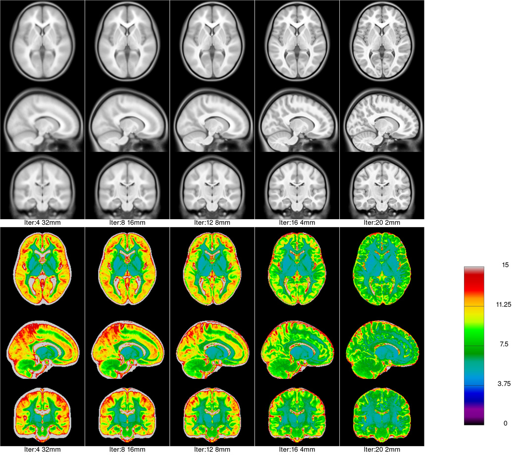
Average asymmetric template (4.5–18.5 y.o.) generated at each level of fitting. The grey scale images show the intensity average anatomy, while the rainbow colour scale shows the intensity standard deviation for selected iterations in the hierarchical fitting process. One can see that as fitting progresses, anatomical features become less blurred and the intensity variability is reduced. The intensity range of the average data sets runs from 0 to 100.

To quantitatively track the convergence of the model, Fig. 4 shows the voxel-wise RMS magnitude of the residual error at each iteration for the asymmetric (black squares) and symmetric (red circles) fitting processes for all NIHPD subjects (4.5–18.5 years). Both curves show similar behavior with respect to the step size and number of iterations, although the displacements are understandably slightly larger for the symmetric model. Another measure of the goodness of fit is the change in the voxel-wise intensity standard deviation, calculated during the averaging of 324 individual warped scans (see Fig. 5). Note how the values of the residual error decrease for a given scale value and then increase at the next scale, before decreasing once again. These jumps are due to the decreases in scale (finer resolution), where more differences are recovered between subjects. If all scans are perfectly normalized, this graph should asymptotically reach the noise level of the acquisitions. The behavior is similar for the creation of the symmetric and asymmetric templates.

Figure 4.

RMS magnitude of the residual error vector field for each iteration (i.e., the bias in the average deformation for the current template), x axis shows the step-size in mm. On the top image, the symmetric (red circles) and asymmetric (black squares) NIHPD 4.5–18.5 models are compared. On the bottom, the different NIHPD age sub-ranges are plotted for the asymmetric atlas creation. One can see that at each iteration for each step size, the average RMS residual error magnitude is reduced, indicating that the optimization procedure is reaching a minima.

Figure 5.

RMS of intensity standard deviation (SD) between individual scans at each iteration for the creation of the NIHPD-4.5–18.5 yo atlas, x axis shows the step-size in mm. As the procedure advances, the RMS intensity SD between iterations decreases progressively for creation of both symmetric (red circles) and asymmetric (black squares) models.

Average anatomy templates

The algorithm was applied to each of the age subgroups of the NIHPD and to the subjects in the ICBM database. Figure 6 shows the final average asymmetric T1w templates for the six NIHPD age ranges and the ICBM young adult population: In each case, the templates provide significant anatomical detail in the central region, cerebellum, brainstem, and cortex, even though a large number of subjects were averaged for each template (e.g., 82 [4.5–8.5 years], 112 [7–11 years], and 152 subjects for the ICBM young adult average). See the T1w pediatric templates in Fig. 7 for better detail.

Figure 6.

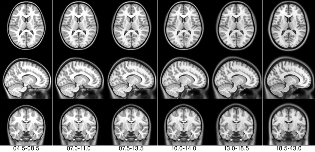
NIHPD asymmetric templates (first six columns) + ICBM asymmetric template (rightmost column) for the T1w modality.

Figure 7.

Close up of the T1w, T2w and PDw (from top to bottom) atlas data to show cortical detail.

For each age-range dataset from the NIHPD and for the subjects in the ICBM database, templates of T2w and PDw modalities were generated (see Fig. 8). In addition, tissue probability maps were created using a genetic tissue classification algorithm on T1w images (Tohka, Krestyannikov et al. 2007), followed by a partial volume effect estimation of the tissue probability maps using all three modalities (T1w, T2w, PDw) (Tohka, Zijdenbos et al. 2004). For each subject, the individual T2w, PDw, and tissue probability maps were warped using the deformation field obtained during the creation of the T1w model, and averaged together to create the average T2w, PDw (c.f. Fig. 8), GM, WM, and CSF tissue probability maps, respectively. Figure 9 shows the tissue probability maps for the full age range of the NIHPD and for all subjects in the ICBM database. Figure 10 shows the detailed GM, WM, and CSF templates for the six age-specific NIHPD pediatric templates and the ICBM young adult template. Figure 11 identifies some anatomical differences between the NIHPD 4.5–8.5 and ICBM 18.5–43.5 templates. The tissue probability maps, brain masks, and the average T1w, T2w, and PDw templates are publicly available in both MINC and NIFTI formats (http://www.bic.mni.mcgill.ca/ServicesAtlases/NIHPD-obj1).

Figure 8.

NIHPD 4.5–18.5 template (left) and ICBM 18.5–43.0 template (right), showing the T1w, T2w and PDw average templates for each group.

Figure 9.

Comparison of probabilistic atlas of the brain tissue types (GM, WM, CSF) for the NIHPD 4.5–18.5 atlas (leftmost 3 columns) and the ICBM 18.5–43.5 atlas (rightmost 3 columns). The brightest voxels indicate high probability of that tissue class. Note that the skin and skull outlines are overlaid on each subimage to facilitate comparisons.

Figure 10.

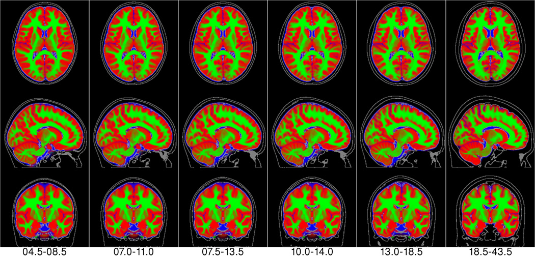
NIHPD templates (leftmost 6 columns) + ICBM template (rightmost column) of the combined tissue class atlas with red representing gray matter; green, white matter and blue color, CSF.

Figure 11.

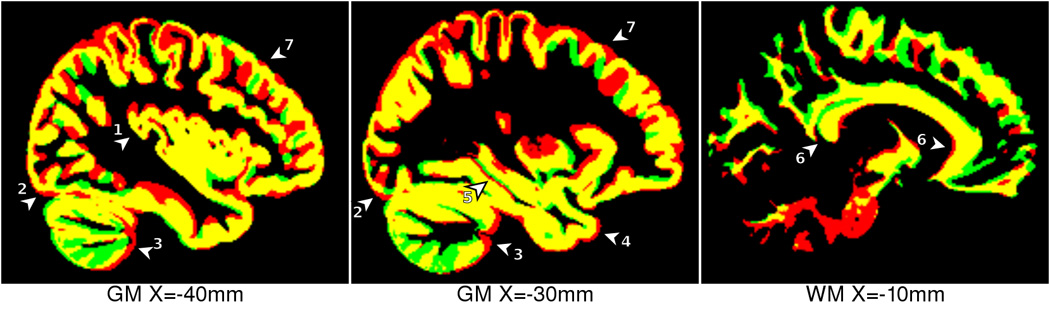
Comparison between NIHPD 4.5–8.5 template (red) and ICBM 18.5–43.5 template (green), overlapping regions in yellow. The following anatomical differences are highlighted: 1) thicker insular cortex in pediatric atlas, 2) more posterior occipital pole in pediatric atlas, 3) different shape and GM/WM ratio in cerebellum, 4) more anterior temporal pole in pediatric atlas, 5) slightly different hippocampal shape, 6) flatter, thinner, longer corpus callosum in adult atlas, 7) thicker GM in pediatric atlas.

Subtle morphological differences between each of these templates (Figs. 6–11) correspond to the maturation of the cerebral anatomy. For example, with all templates normalized to the same overall brain size, with age the corpus callosum thins, flattens slightly and lengthens slightly in the AP direction (Figs 11 & 12). In addition, the lateral ventricles increase in size and the sulcal spaces widen in adulthood. In the frontal lobe, the ratio of WM to GM appears to increase with age. Further, the basal ganglia and thalamus appear wider and longer with increasing age, the pons enlarges with age and the posterior part of the brain (cerebellum and occipital pole) appears to shift in the superior direction, with the cerebellum widening with age (See Fig 12).

Figure 12.

Comparison between NIHPD 4.5–8.5 and ICBM 18.5–43.5 templates. When compared to the the ICBM atlas, the NIHPD 4.5–8.5 atlas has thinner skull and scalp, narrower cortical suci (A = Post Central Sulcus, B = Parieto-Occipital Sulcus, C = Calcarine Fissure), decreased separation of the cerebellar folia (D), thinner corpus callosum (E), smaller lateral ventricles (F), and thicker cortex overall, Internal architecture of the thalamus has a slightly different shape (G), Different shape of the pituitary gland (H), and the presence of the spheno-occipital synchondrosis (I), smaller pons (J).

Deformation-based morphometry example study

As an example of the potential effect the choice of template can have on analysis, a DBM study of the youngest subjects from the NIHPD was completed using four different target templates: the 7.0–11.0 years, the 10.0–14.0 years, and the 13.0–18.5 years NIHPD atlas templates as well as the ICBM young adult atlas template. The test set included subjects in the age range of 4.5–6.9 years that passed MRI quality control with the primary acquisition sequence and thus were comparable to the atlas templates (n = 66 subjects). The objective here was not to complete a full DBM study, but rather to quantify the differences (or potential bias) that choice of template might have on eventual analysis. The templates are compared in a pair-wise fashion such that one template (7.0–11.0 years) is close to the appropriate age of the subjects and the second template is selected from the remaining three that are further away in age. These results clearly show that the bias (or difference) between templates increases as the difference in average age between templates is increased.

Each of the T1w MRI volumes in the test set was processed four times according to the standard data preprocessing steps (as described above), each time using one of the four aforementioned templates. After preprocessing, the nonlinear registration algorithm ANIMAL was used to estimate the mapping between each template and the preprocessed, brain-masked, linearly transformed data for each of the test subjects. This procedure yielded 66 × 4 deformation fields.

The Jacobian determinant J was estimated for each node in each deformation field. The log Jacobian was computed, producing four fields of the local volume difference, logJ_{NIHPD-7.0–11.0}, logJ_{NIHPD-10.0–14.0}, logJ_{NIHPD-13.0–18.5}, and logJ_ICBM, for each subject of the test set. As the log Jacobian maps are defined in the space of the templates, for comparison, they need to be transformed into a common space. All NIHPD log Jacobian maps were transformed through the nonlinear deformation, by which each NIHPD template was mapped to the space of the ICBM template for analysis. A voxel-wise, pair-wise Student‘s t-test was then performed on the absolute difference from 0.0 between the resampled logJ_{NIHPD-7.0–11.0} and the logJ_{NIHPD-10.0–14.0}, logJ_{NIHPD-13.0–18.5} and the logJ_ICBM templates. To account for the multiple-comparisons we have used False Discovery Rate (FDR) of 5% to calculate threshold for statistically significant differences (Genovese, Lazar et al. 2002).

Since the test subjects are not draw from the same age range as the target templates, the average log Jacobian map is not expected to be null. This is indeed the case, and for each template, the average magnitude of the deformation bias increases with age. The results of the Student‘s t-test shown in Fig. 13 demonstrate regions where this bias is significantly (corrected for multiple comparisons, FDR=5%) different between pairs of templates. When the age difference between templates is small, for example when logJ_{NIHPD-7.0–11.0} and logJ_{NIHPD-10.0–14.0} are compared, the potentially biased regions are quite small and focused near the center of the brain. However, as the age between the templates increases, the size of the significantly different regions increases as well. When an adult template is used to analyze a pediatric dataset in the 4.5–6.9y range, there is a systematic bias in the estimation of tissue growth or shrinkage in the central regions of the brain, particularly around the ventricles. This result is not surprising, given the different appearance of the ventricles and the corpus callosum in these templates (see Fig. 6, Fig 11).

Figure 13.

Regions of potential bias when using different atlases. Map of statistically significant differences in log Jacobians when mapping the NIHPD 4.5–6.9 age group to the NIHPD 7.0–11.0 (baseline for comparison) and the NIHPD 10.0–14.0 (top row), NIHPD13.0–18.5 (middle row) and ICBM18.5–45.0 (bottom row) templates, all presented in the space of the ICBM 18.5–45.0 template. Red color indicates regions where the selected templates produces significantly (5% False Discovery Rate (Genovese, Lazar et al. 2002)) bigger log Jacobian determinant (i.e., a significant difference in local volume) compared to the NIHPD 7.0–11.0 template, and blue color indicates where the selected template yields a statistically significant smaller Jacobian determinant. One can see that the red regions are much larger than the blue regions, indicating potential bias non-age appropriate template for analysis of pediatric data in the 4.5–6.9y range

Discussion

On the method

We have developed and characterized a method of creating unbiased symmetric and asymmetric templates of MRI data from large ensembles of subjects. Our method uses iterative refinement with successively finer scales of nonlinear registration to yield templates with a high degree of anatomical detail, even at the cortex. For this paper, we created unbiased symmetric and asymmetric templates of pediatric data for six (overlapping) age ranges, using MRI data available to qualified researchers from the NIH MRI Study of Normal Brain Development. For comparison, we built a young adult template from MRI data from 152 young adults who had participated in the ICBM project (Mazziotta, Toga et al. 1995). In each case, the templates include nonlinear averages of T1w, T2w, and PDw images, average brain masks, and average GM, WM, and CSF maps. These atlases are publicly available from http://www.bic.mni.mcgill.ca/ServicesAtlases, where they can be viewed and downloaded.

Results of the iterative averaging procedure demonstrate that it is possible to generate average maps of anatomy from large numbers of subjects and retain detail not only for the central region of the brain, but also at the cortex (see Figs. 6–10). Figures 3–5 show that the iterative process behaves well and converges with a small number of iterations.

On the atlases

The templates were created for specific age ranges of subjects, selected from a epidemiological sample of normal healthy children 4.5–18.5 years old, that are representative of the U.S. population and have been carefully screened for medical and psychiatric factors and have been characterized using a series of standardized rating scales, cognitive tests and interviews. The use of such a cohort makes these templates practically useful for both clinical and more basic research in pediatric studies.

The generated symmetric and asymmetric templates should enable better unbiased analyses of pediatric data, with each type of template appropriate for certain types of analysis. For example, a symmetric template is better suited to analyze left–right differences in a particular population, whereas the asymmetric templates should be used as registration targets for all other studies where left–right comparison is not the major goal. In addition, one only has to manually segment one side of the brain when building a symmetric segmentation atlas.

Not surprisingly, our DBM study demonstrated that different templates give rise to different results; therefore, using an adult template for pediatric data will yield different results than an age-appropriate template. Furthermore, comparisons between templates showed that this variation increases as the average age between templates increases. Experiments with the test set demonstrated that using an atlas close to the appropriate age yields fewer regions of potential bias than using an adult atlas. Indeed, Fig. 13 shows large regions where the deformation field is different from 1.0, indicating regions where the atlas is, on average, either larger or smaller than the corresponding regions of the internal test subjects. Since the experiments presented here only show that a difference exists, it is not possible to judge which template is preferable; selection of the best template will be task-specific. However, one might assume that a more accurate template (in terms of average morphometry) is better.

Comparison to other atlas building strategies

Our atlas-building strategy bears some similarities to previous iterative methods (Guimond, Meunier et al. 1998) (Guimond, Meunier et al. 2000); (Guimond, Meunier et al. 2000); (Joshi, Davis et al. 2004); (Bhatia, Aljabar et al. 2007), but with some important differences: For example, in Guimond et al. (Guimond, Meunier et al. 1998; Guimond, Meunier et al. 2000), the subject was registered to a template, and the deformations were averaged, inverted, and then applied to the average resampled data to remove bias. Here, we compute the deformations from the template to each subject, after linear registration in stereotaxic space, to allow estimation of the nonlinear deformation in the template space and justify vector averaging. Grabner et al. (Grabner, Janke et al. 2006) extended the work of Guimond et al. to include steps to build a symmetric template similar to those we use here. However, in contrast to both Guimond and Grabner, who used tri-linear interpolation to resample the MRI data, we use spline interpolation to yield slightly better results (Thévenaz, Blu et al. 2000). Guimond and Grabner also start from scratch at each iteration; that is, at iteration n, they recompute the registration steps 0, 1…n, where iteration 0 is a linear transformation to the target, whereas we use the transformation computed at iteration n−1 as the starting point for iteration n, which helps maintain the stability of the process. Moreover, unlike Joshi et al. (Joshi, Davis et al. 2004), who used a large deformation diffeomorphic fluid approach that integrates streamlines (i.e., velocity field integration) into the deformation averaging approach, our work (and that of Guimond and Grabner) uses a linear elastic model, enabling a simpler averaging of vectors to estimate the mean deformation field. Finally, Bhatia et al. (Bhatia, Aljabar et al. 2007) alternated group-wise combined segmentation and B-spline registration of the tissue classes in a global optimization procedure to form the templates. By contrast, our technique fits T1 intensities directly using a local optimization registration procedure.

Whereas we average data from all subjects within a group, the Template-O-Matic method (Wilke (Wilke, Holland et al. 2008) uses statistical analysis to compute weights of affine-registered GM and WM maps from each subject to generate customized tissue map templates that match a particular pediatric population under study. This differs from our method, where (1) age ranges are predefined according to hypotheses regarding aspects of brain development and (2) nonlinear iterative registration is used to align all datasets. The latter results in the much clearer and sharper average tissue templates seen in Fig. 9, compared to Fig. 3 of Wilke (Wilke, Holland et al. 2008). Still, the statistical subject-weighting scheme deserves further investigation to determine, for instance, if it can be combined with a nonlinear registration scheme similar to that described here.

A number of factors complicate the direct comparison of our template results with those published previously, including differences between the MRI data quality and number of subjects used to build the templates, the particular population studied, alignment method, registration strategy, scale of the deformation, and different metrics reported. With these caveats in mind, we compare our template results with those in the literature: Shan et al. (Shan, Parra et al. 2006) created an atlas from the anatomy of a single 9-year-old subject. The atlases of Jelacic et al. (Jelacic, de Regt et al. 2006) allow the comparison of the anatomy of a given subject with those of other subjects, manually selected from a small group of standard normal scans. Kochunov et al. (Kochunov, Lancaster et al. 2001), Park et al.(Park, Bland et al. 2005), and Wu et al. (Wu, Rosano et al. 2007) all described methods to select the best template from a collection of potential MRI scans. As a justification for using a single subject atlas, they cited the blurred appearance of older average templates such as the MNI305 or ICBM152, which were created using only linear transformations. However, while a single subject template may be a good match globally for a specific subject under study, it is still possible that some local region of the template might represent an extreme of the normal distribution, which could potentially result in a biased analysis. Furthermore, when studying groups of subjects, it is necessary to align all subjects into a common coordinate space. With the best template strategy, this is impossible because there is a different best template for every subject being studied. By contrast, the atlases presented here represent the average anatomy of large groups of subjects; thus, they are less biased than atlases created from single subjects. In addition, the same template can be used as a common registration target for studies involving multiple subjects. Finally, the iterative nonlinear registration strategy used here results in templates with high anatomical detail throughout the brain, thus obviating the need to justify the use of a single subject atlas for registration.

As far as multi-subject atlases, Joshi et al. (Joshi, Davis et al. 2004), Kazemi et al. (Kazemi, Moghaddam et al. 2007), and Bhatia et al. (Bhatia, Aljabar et al. 2007) created atlases from eight, seven, and 22 subjects, respectively. Though an improvement on single subject templates, these atlases used substantially fewer subjects than those described here. Finally, these dedicated atlases represent the anatomy from a small, limited age range, whereas our atlases span ages from 4.5 to 43.5 years. Qualitatively, the atlas presented in Fig. 4 of Joshi et al. (Joshi, Davis et al. 2004) and that presented in Figs. 1 and 2 of Bhatia et al. (Bhatia, Aljabar et al. 2007) appear to have slightly less detail in the cortex than the atlases presented here, perhaps due to the larger number and the (older) ages of subjects used to create our templates.

In conclusion, we have presented a method for unbiased atlas generation from large ensembles of MRI data. We have demonstrated that the iterative method converges and the resulting atlas templates maintain high anatomical detail throughout the brain. These publicly available templates are derived from a truly normal, well characterized population and should facilitate spatial normalization and image analysis for better understanding of pediatric populations.

Appendix A: Brain Development Cooperative Group

The MRI Study of Normal Brain Development is a cooperative study performed by six pediatric study centers in collaboration with a Data Coordinating Center (DCC), a Clinical Coordinating Center (CCC), a Diffusion Tensor Processing Center (DPC), and staff of the National Institute of Child Health and Human Development (NICHD), the National Institute of Mental Health (NIMH), the National Institute for Drug Abuse (NIDA), and the National Institute for Neurological Diseases and Stroke (NINDS), Rockville, Maryland. Key personnel from the six pediatric study centers are as follows: Children‘s Hospital Medical Center of Cincinnati, Principal Investigator William S. Ball, M.D., Investigators Anna Weber Byars, Ph.D., Mark Schapiro, M.D., Wendy Bommer, R.N., April Carr, B.S., April German, B.A., Scott Dunn, R.T.; Children‘s Hospital Boston, Principal Investigator Michael J. Rivkin, M.D., Investigators Deborah Waber, Ph.D., Robert Mulkern, Ph.D., Sridhar Vajapeyam, Ph.D., Abigail Chiverton, B.A., Peter Davis, B.S., Julie Koo, B.S., Jacki Marmor, M.A., Christine Mrakotsky, Ph.D., M.A., Richard Robertson, M.D., Gloria McAnulty, Ph.D.; University of Texas Health Science Center at Houston, Principal Investigators Michael E. Brandt, Ph.D., Jack M. Fletcher, Ph.D., Larry A. Kramer, M.D., Investigators Grace Yang, M.Ed., Cara McCormack, B.S., Kathleen M. Hebert, M.A., Hilda Volero, M.D.; Washington University in St. Louis, Principal Investigators Kelly Botteron, M.D., Robert C. McKinstry, M.D., Ph.D., Investigators William Warren, Tomoyuki Nishino, M.S., C. Robert Almli, Ph.D., Richard Todd, Ph.D., M.D., John Constantino, M.D.; University of California Los Angeles, Principal Investigator James T. McCracken, M.D., Investigators Jennifer Levitt, M.D., Jeffrey Alger, Ph.D., Joseph O'Neil, Ph.D., Arthur Toga, Ph.D., Robert Asarnow, Ph.D., David Fadale, B.A., Laura Heinichen, B.A., Cedric Ireland B.A.; Children‘s Hospital of Philadelphia, Principal Investigators Dah-Jyuu Wang, Ph.D. and Edward Moss, Ph.D., Investigator Robert A. Zimmerman, M.D., and Research Staff Brooke Bintliff, B.S., Ruth Bradford, Janice Newman, M.B.A. The Principal Investigator of the data coordinating center at McGill University is Alan C. Evans, Ph.D., Investigators Rozalia Arnaoutelis, B.S., G. Bruce Pike, Ph.D., D. Louis Collins, Ph.D., Gabriel Leonard, Ph.D., Tomas Paus, M.D., Alex Zijdenbos, Ph.D., and Research Staff Samir Das, B.S., Vladimir Fonov, Ph.D., Luke Fu, B.S., Jonathan Harlap, Ilana Leppert, B.E., Denise Milovan, M.A., Dario Vins, B.C., and at Georgetown University, Thomas Zeffiro, M.D., Ph.D. and John Van Meter, Ph.D. Investigators at the Neurostatistics Laboratory, Harvard University/McLean Hospital, Nicholas Lange, Sc.D. and Michael P. Froimowitz, M.S., work with data coordinating center staff and all other team members on biostatistical study design and data analyses. The Principal Investigator of the Clinical Coordinating Center at Washington University is Kelly Botteron, M.D., Investigators C. Robert Almli, Ph.D., Cheryl Rainey, B.S., Stan Henderson, M.S., Tomoyuki Nishino, M.S., William Warren, Jennifer L. Edwards, M.SW., Diane Dubois, R.N., Karla Smith, Tish Singer and Aaron A. Wilber, M.S. The Principal Investigator of the Diffusion Tensor Processing Center at the National Institutes of Health is Carlo Pierpaoli, M.D., Ph.D., Investigators Peter J. Basser, Ph.D., Lin-Ching Chang, Sc.D., Chen Guan Koay, Ph.D. and Lindsay Walker, M.S. The Principal Collaborators at the National Institutes of Health are Lisa Freund, Ph.D. (NICHD), Judith Rumsey, Ph.D. (NIMH), Lauren Baskir, Ph.D. (NIMH), Laurence Stanford, Ph.D. (NIDA), Karen Sirocco, Ph.D. (NIDA) and from NINDS, Katrina Gwinn-Hardy, M.D. and Giovanna Spinella, M.D. The Principal Investigator of the Spectroscopy Processing Center at the University of California Los Angeles is James T. McCracken, M.D., Investigators Jeffry R. Alger, Ph.D., Jennifer Levitt, M.D., Joseph O'Neill, Ph.D.

References

- Almli CR, Rivkin MJ, et al. The NIH MRI study of normal brain development (Objective-2): Newborns, infants, toddlers, and preschoolers. Neuroimage. 2007;35(1):308–325. doi: 10.1016/j.neuroimage.2006.08.058. [DOI] [PubMed] [Google Scholar]
- Amit Y, Grenander U, et al. Structural Image Restoration Through Deformable Templates. Journal of the American Statistical Association. 1991;86(414):376–387. [Google Scholar]
- Ardekani BA, Guckemus S, et al. Quantitative comparison of algorithms for inter-subject registration of 3D volumetric brain MRI scans. Journal of Neuroscience Methods. 2005;142(1):67–76. doi: 10.1016/j.jneumeth.2004.07.014. [DOI] [PubMed] [Google Scholar]
- Arsigny V, Commowick O, et al. A Log-Euclidean Framework for Statistics on Diffeomorphisms. Medical Image Computing and Computer-Assisted Intervention – MICCAI 2006. 2006:924–931. doi: 10.1007/11866565_113. [DOI] [PubMed] [Google Scholar]
- Ashburner J, Friston K. Multimodal Image Coregistration and Partitioning--A Unified Framework. NeuroImage. 1997;6(3):209–217. doi: 10.1006/nimg.1997.0290. [DOI] [PubMed] [Google Scholar]
- Avants B, Grossman M, et al. Symmetric Diffeomorphic Image Registration: Evaluating Automated Labeling of Elderly and Neurodegenerative Cortex and Frontal Lobe. Biomedical Image Registration. 2006:50–57. doi: 10.1016/j.media.2007.06.004. [DOI] [PMC free article] [PubMed] [Google Scholar]
- Avants BB, Epstein CL, et al. Symmetric diffeomorphic image registration with cross-correlation: Evaluating automated labeling of elderly and neurodegenerative brain. Medical Image Analysis. 2008;12(1):26–41. doi: 10.1016/j.media.2007.06.004. [DOI] [PMC free article] [PubMed] [Google Scholar]
- Bartzokis G, Beckson M, et al. Age-related changes in frontal and temporal lobe volumes in men: a magnetic resonance imaging study. Arch Gen Psychiatry. 2001;58(5):461–465. doi: 10.1001/archpsyc.58.5.461. [DOI] [PubMed] [Google Scholar]
- Bhatia K, Aljabar P, et al. Groupwise Combined Segmentation and Registration for Atlas Construction. Medical Image Computing and Computer-Assisted Intervention – MICCAI 2007. 2007:532–540. doi: 10.1007/978-3-540-75757-3_65. [DOI] [PubMed] [Google Scholar]
- Bhatia KK, Hajnal JV, et al. Consistent groupwise non-rigid registration for atlas construction. Biomedical Imaging: Nano to Macro, 2004. IEEE International Symposium on.2004. [Google Scholar]
- Blanton RE, Levitt JG, et al. Gender differences in the left inferior frontal gyrus in normal children. Neuroimage. 2004;22(2):626–636. doi: 10.1016/j.neuroimage.2004.01.010. [DOI] [PubMed] [Google Scholar]
- Blanton RE, Levitt JG, et al. Mapping cortical asymmetry and complexity patterns in normal children. Psychiatry Res. 2001;107(1):29–43. doi: 10.1016/s0925-4927(01)00091-9. [DOI] [PubMed] [Google Scholar]
- Blatter DD, Bigler ED, et al. Quantitative volumetric analysis of brain MR: normative database spanning 5 decades of life. AJNR Am J Neuroradiol. 1995;16(2):241–251. [PMC free article] [PubMed] [Google Scholar]
- Carmichael OT, Aizenstein HA, et al. Atlas-based hippocampus segmentation in Alzheimer's disease and mild cognitive impairment. Neuroimage. 2005;27(4):979–990. doi: 10.1016/j.neuroimage.2005.05.005. [DOI] [PMC free article] [PubMed] [Google Scholar]
- Caviness VS, Jr, Kennedy DN, et al. The human brain age 7–11 years: a volumetric analysis based on magnetic resonance images. Cereb Cortex. 1996;6(5):726–736. doi: 10.1093/cercor/6.5.726. [DOI] [PubMed] [Google Scholar]
- Caviness VS, Jr, Lange NT, et al. MRI-based brain volumetrics: emergence of a developmental brain science. Brain Dev. 1999;21(5):289–295. doi: 10.1016/s0387-7604(99)00022-4. [DOI] [PubMed] [Google Scholar]
- Christensen GE, Rabbitt RD, et al. 3D brain mapping using a deformable neuroanatomy. Physics in Medicine and Biology. 1994;39(3):609–618. doi: 10.1088/0031-9155/39/3/022. [DOI] [PubMed] [Google Scholar]
- Chung MK, Worsley KJ, et al. A Unified Statistical Approach to Deformation-Based Morphometry. NeuroImage. 2001;14(3):595–606. doi: 10.1006/nimg.2001.0862. [DOI] [PubMed] [Google Scholar]
- Collins DL, Neelin P, et al. Automatic 3D intersubject registration of MR volumetric data in standardized Talairach space. Journal of Computer Assisted Tomography. 1994;18(2):192–205. [PubMed] [Google Scholar]
- Collins DL, Zijdenbos AP, et al. ANIMAL+INSECT: Improved Cortical Structure Segmentation. Information Processing in Medical Imaging: 16th International Conference, IPMI'99; Visegrád, Hungary. 1999. [June/July 1999]. Proceedings: 210. [Google Scholar]
- Courchesne E, Chisum HJ, et al. Normal brain development and aging: quantitative analysis at in vivo MR imaging in healthy volunteers. Radiology. 2000;216(3):672–682. doi: 10.1148/radiology.216.3.r00au37672. [DOI] [PubMed] [Google Scholar]
- De Bellis MD, Keshavan MS, et al. Sex differences in brain maturation during childhood and adolescence. Cereb Cortex. 2001;11(6):552–557. doi: 10.1093/cercor/11.6.552. [DOI] [PubMed] [Google Scholar]
- Durston S, Hulshoff Pol HE, et al. Anatomical MRI of the developing human brain: what have we learned? J Am Acad Child Adolesc Psychiatry. 2001;40(9):1012–1020. doi: 10.1097/00004583-200109000-00009. [DOI] [PubMed] [Google Scholar]
- Essen V, D C. Windows on the brain: the emerging role of atlases and databases in neuroscience. Current Opinion in Neurobiology. 2002;12(5):574–579. doi: 10.1016/s0959-4388(02)00361-6. [DOI] [PubMed] [Google Scholar]
- Essen V, David C. A Population-Average, Landmark- and Surface-based (PALS) atlas of human cerebral cortex. NeuroImage. 2005;28(3):635–662. doi: 10.1016/j.neuroimage.2005.06.058. [DOI] [PubMed] [Google Scholar]
- Evans AC, Collins DL, et al. 3D statistical neuroanatomical models from 305 MRI volumes. Nuclear Science Symposium and Medical Imaging Conference, 1993; 1993 IEEE Conference Record.1993. [Google Scholar]
- B. D. C. Group. Evans AC. The NIH MRI study of normal brain development. NeuroImage. 2006;30(1):184–202. doi: 10.1016/j.neuroimage.2005.09.068. [DOI] [PubMed] [Google Scholar]
- Filipek PA, Richelme C, et al. The young adult human brain: an MRI-based morphometric analysis. Cereb Cortex. 1994;4(4):344–360. doi: 10.1093/cercor/4.4.344. [DOI] [PubMed] [Google Scholar]
- Genovese CR, Lazar NA, et al. Thresholding of Statistical Maps in Functional Neuroimaging Using the False Discovery Rate. Neuroimage. 2002;15(4):870–878. doi: 10.1006/nimg.2001.1037. [DOI] [PubMed] [Google Scholar]
- Gerig G, Davis B, et al. Computational Anatomy to Assess Longitudinal Trajectory of Brain Growth. 3D Data Processing, Visualization, and Transmission, Third International Symposium on.2006. [Google Scholar]
- Giedd JN, Blumenthal J, et al. Brain development during childhood and adolescence: a longitudinal MRI study. Nat Neurosci. 1999;2(10):861–863. doi: 10.1038/13158. [DOI] [PubMed] [Google Scholar]
- Giedd JN, Rumsey JM, et al. A quantitative MRI study of the corpus callosum in children and adolescents. Brain Res Dev Brain Res. 1996;91(2):274–280. doi: 10.1016/0165-3806(95)00193-x. [DOI] [PubMed] [Google Scholar]
- Giedd JN, Vaituzis AC, et al. Quantitative MRI of the temporal lobe, amygdala, and hippocampus in normal human development: ages 4–18 years. J Comp Neurol. 1996;366(2):223–230. doi: 10.1002/(SICI)1096-9861(19960304)366:2<223::AID-CNE3>3.0.CO;2-7. [DOI] [PubMed] [Google Scholar]
- Gogtay N, Giedd J, et al. Brain development in healthy, hyperactive, and psychotic children. Arch Neurol. 2002;59(8):1244–1248. doi: 10.1001/archneur.59.8.1244. [DOI] [PubMed] [Google Scholar]
- Gogtay N, Giedd JN, et al. Dynamic mapping of human cortical development during childhood through early adulthood. Proc Natl Acad Sci U S A. 2004;101(21):8174–8179. doi: 10.1073/pnas.0402680101. [DOI] [PMC free article] [PubMed] [Google Scholar]
- Good CD, Johnsrude IS, et al. A voxel-based morphometric study of ageing in 465 normal adult human brains. Neuroimage. 2001;14(1 Pt 1):21–36. doi: 10.1006/nimg.2001.0786. [DOI] [PubMed] [Google Scholar]
- Grabner G, Janke AL, et al. Symmetric atlasing and model based segmentation: an application to the hippocampus in older adults. Med Image Comput Comput Assist Interv Int Conf Med Image Comput Comput Assist Interv. 2006;9(Pt 2):58–66. doi: 10.1007/11866763_8. [DOI] [PubMed] [Google Scholar]
- Guimond A, Meunier J, et al. Automatic Computation of Average Brain Models. Medical Image Computing and Computer-Assisted Interventation — MICCAI’98. 1998:631. [Google Scholar]
- Guimond A, Meunier J, et al. Average Brain Models: A Convergence Study. Computer Vision and Image Understanding. 2000;77:192–210. [Google Scholar]
- Guimond A, Roche A, et al. Three-dimensional multimodal brain warping using the demons algorithm and adaptive intensity corrections. IEEE Trans Med Imaging. 2001;20(1):58–69. doi: 10.1109/42.906425. [DOI] [PubMed] [Google Scholar]
- Guizzard N, Fonov V, et al. Symmetric Optimization Scheme versus Constrained Symmetrization for Non-Linear Registrations. MICCAI workshop on “Medical Image Analysis on Multiple Sclerosis (validation and methodological issues)”. 2009 [Google Scholar]
- Hoeksma MR, Kenemans JL, et al. Variability in spatial normalization of pediatric and adult brain images. Clinical Neurophysiology. 2005;116(5):1188–1194. doi: 10.1016/j.clinph.2004.12.021. [DOI] [PubMed] [Google Scholar]
- Janke A, Evans A, et al. MNI- and Talairach- space: Everything you wanted to know but were afraid to ask. Florence, Italy: HBM; 2006. [Google Scholar]
- Jelacic S, de Regt D, et al. Interactive Digital MR Atlas of the Pediatric Brain. Radiographics. 2006;26(2):497–501. doi: 10.1148/rg.262055009. [DOI] [PubMed] [Google Scholar]
- Jernigan TL, Tallal P. Late childhood changes in brain morphology observable with MRI. Dev Med Child Neurol. 1990;32(5):379–385. doi: 10.1111/j.1469-8749.1990.tb16956.x. [DOI] [PubMed] [Google Scholar]
- Jernigan TL, Trauner DA, et al. Maturation of human cerebrum observed in vivo during adolescence. Brain. 1991;114(Pt 5):2037–2049. doi: 10.1093/brain/114.5.2037. [DOI] [PubMed] [Google Scholar]
- Joshi S, Davis B, et al. Unbiased diffeomorphic atlas construction for computational anatomy. Neuroimage. 2004;23 Suppl 1:S151–S160. doi: 10.1016/j.neuroimage.2004.07.068. [DOI] [PubMed] [Google Scholar]
- Joshi SC, Miller MI. Landmark matching via large deformation diffeomorphisms. Image Processing, IEEE Transactions on. 2000;9(8):1357–1370. doi: 10.1109/83.855431. [DOI] [PubMed] [Google Scholar]
- Kazemi K, Moghaddam HA, et al. A neonatal atlas template for spatial normalization of whole-brain magnetic resonance images of newborns: Preliminary results. NeuroImage. 2007;37(2):463–473. doi: 10.1016/j.neuroimage.2007.05.004. [DOI] [PubMed] [Google Scholar]
- Kennedy DN, Haselgrove C, et al. MRI-based morphometric of typical and atypical brain development. Ment Retard Dev Disabil Res Rev. 2003;9(3):155–160. doi: 10.1002/mrdd.10075. [DOI] [PubMed] [Google Scholar]
- Kennedy DN, Lange N, et al. Gyri of the human neocortex: an MRI-based analysis of volume and variance. Cereb Cortex. 1998;8(4):372–384. doi: 10.1093/cercor/8.4.372. [DOI] [PubMed] [Google Scholar]
- Klein A, Andersson J, et al. Evaluation of 14 nonlinear deformation algorithms applied to human brain MRI registration. Neuroimage. 2009;46(3):786–802. doi: 10.1016/j.neuroimage.2008.12.037. [DOI] [PMC free article] [PubMed] [Google Scholar]
- Kochunov P, Lancaster JL, et al. Regional spatial normalization: toward an optimal target. J Comput Assist Tomogr. 2001;25(5):805–816. doi: 10.1097/00004728-200109000-00023. [DOI] [PubMed] [Google Scholar]
- Lange N, Giedd JN, et al. Variability of human brain structure size: ages 4–20 years. Psychiatry Res. 1997;74(1):1–12. doi: 10.1016/s0925-4927(96)03054-5. [DOI] [PubMed] [Google Scholar]
- Lorenzen P, Davis B, et al. Unbiased atlas formation via large deformations metric mapping. Med Image Comput Comput Assist Interv Int Conf Med Image Comput Comput Assist Interv. 2005;8(Pt 2):411–418. doi: 10.1007/11566489_51. [DOI] [PubMed] [Google Scholar]
- Lorenzen PJ, Joshi SC. High-dimensional multi-modal image registration. 2003;2717:234–243. [Google Scholar]
- Machilsen B, d'Agostino E, et al. Linear normalization of MR brain images in pediatric patients with periventricular leukomalacia. NeuroImage. 2007;35(2):686–697. doi: 10.1016/j.neuroimage.2006.12.037. [DOI] [PubMed] [Google Scholar]
- Mazziotta J, Toga A, et al. A probabilistic atlas and reference system for the human brain: International Consortium for Brain Mapping (ICBM) Philosophical Transactions of the Royal Society B: Biological Sciences. 2001;356(1412):1293–1322. doi: 10.1098/rstb.2001.0915. [DOI] [PMC free article] [PubMed] [Google Scholar]
- Mazziotta J, Toga A, et al. A four-dimensional probabilistic atlas of the human brain. J Am Med Inform Assoc. 2001;8(5):401–430. doi: 10.1136/jamia.2001.0080401. [DOI] [PMC free article] [PubMed] [Google Scholar]
- Mazziotta JC, Toga AW, et al. A probabilistic atlas of the human brain: theory and rationale for its development. The International Consortium for Brain Mapping (ICBM) Neuroimage. 1995;2(2):89–101. doi: 10.1006/nimg.1995.1012. [DOI] [PubMed] [Google Scholar]
- Miller M, Banerjee A, et al. Statistical methods in computational anatomy. Stat Methods Med Res. 1997;6(3):267–299. doi: 10.1177/096228029700600305. [DOI] [PubMed] [Google Scholar]
- Muzik O, Chugani DC, et al. Statistical Parametric Mapping: Assessment of Application in Children. Neuroimage. 2000:538–549. doi: 10.1006/nimg.2000.0651. [DOI] [PubMed] [Google Scholar]
- Nyul LG, Udupa JK. On standardizing the MR image intensity scale. Magn Reson Med. 1999;42(6):1072–1081. doi: 10.1002/(sici)1522-2594(199912)42:6<1072::aid-mrm11>3.0.co;2-m. [DOI] [PubMed] [Google Scholar]
- Park H, Bland PH, et al. Least Biased Target Selection in Probabilistic Atlas Construction. Medical Image Computing and Computer-Assisted Intervention – MICCAI 2005. 2005:419–426. doi: 10.1007/11566489_52. [DOI] [PubMed] [Google Scholar]
- Paus T, Zijdenbos A, et al. Structural maturation of neural pathways in children and adolescents: in vivo study. Science. 1999;283(5409):1908–1911. doi: 10.1126/science.283.5409.1908. [DOI] [PubMed] [Google Scholar]
- Petersen AC, Crockett L, et al. A self-report measure of pubertal status: Reliability, validity, and initial norms. Journal of Youth and Adolescence. 1988;17(2):117–133. doi: 10.1007/BF01537962. [DOI] [PubMed] [Google Scholar]
- Pfefferbaum A, Mathalon DH, et al. A quantitative magnetic resonance imaging study of changes in brain morphology from infancy to late adulthood. Arch Neurol. 1994;51(9):874–887. doi: 10.1001/archneur.1994.00540210046012. [DOI] [PubMed] [Google Scholar]
- Reiss AL, Abrams MT, et al. Brain development, gender and IQ in children. A volumetric imaging study. Brain. 1996;119(Pt 5):1763–1774. doi: 10.1093/brain/119.5.1763. [DOI] [PubMed] [Google Scholar]
- Seghers D, D‘Agostino E, et al. Construction of a Brain Template from MR Images Using State-of-the-Art Registration and Segmentation Techniques. Medical Image Computing and Computer-Assisted Intervention – MICCAI 2004. 2004:696–703. [Google Scholar]
- Shan Z, Parra C, et al. A Digital Pediatric Brain Structure Atlas from T1-Weighted MR Images. Medical Image Computing and Computer-Assisted Intervention – MICCAI 2006. 2006:332–339. doi: 10.1007/11866763_41. [DOI] [PubMed] [Google Scholar]
- Shattuck DW, Mirza M, et al. Construction of a 3D probabilistic atlas of human cortical structures. Neuroimage. 2008;39(3):1064–1080. doi: 10.1016/j.neuroimage.2007.09.031. [DOI] [PMC free article] [PubMed] [Google Scholar]
- Sled JG, Zijdenbos AP, et al. A nonparametric method for automatic correction of intensity nonuniformity in MRI data. Medical Imaging, IEEE Transactions on. 1998;17(1):87–97. doi: 10.1109/42.668698. [DOI] [PubMed] [Google Scholar]
- Smith SM. Fast robust automated brain extraction. Hum Brain Mapp. 2002;17(3):143–155. doi: 10.1002/hbm.10062. [DOI] [PMC free article] [PubMed] [Google Scholar]
- Smith SM, Jenkinson M, et al. Advances in functional and structural MR image analysis and implementation as FSL. Neuroimage. 2004;23:S208–S219. doi: 10.1016/j.neuroimage.2004.07.051. [DOI] [PubMed] [Google Scholar]
- Sowell ER, Peterson BS, et al. Mapping cortical change across the human life span. Nat Neurosci. 2003;6(3):309–315. doi: 10.1038/nn1008. [DOI] [PubMed] [Google Scholar]
- Sowell ER, Thompson PM, et al. Localizing age-related changes in brain structure between childhood and adolescence using statistical parametric mapping. Neuroimage. 1999;9(6 Pt 1):587–597. doi: 10.1006/nimg.1999.0436. [DOI] [PubMed] [Google Scholar]
- Sowell ER, Thompson PM, et al. Longitudinal mapping of cortical thickness and brain growth in normal children. J Neurosci. 2004;24(38):8223–8231. doi: 10.1523/JNEUROSCI.1798-04.2004. [DOI] [PMC free article] [PubMed] [Google Scholar]
- Sowell ER, Thompson PM, et al. Mapping sulcal pattern asymmetry and local cortical surface gray matter distribution in vivo: maturation in perisylvian cortices. Cereb Cortex. 2002;12(1):17–26. doi: 10.1093/cercor/12.1.17. [DOI] [PubMed] [Google Scholar]
- Sowell ER, Thompson PM, et al. Mapping changes in the human cortex throughout the span of life. Neuroscientist. 2004;10(4):372–392. doi: 10.1177/1073858404263960. [DOI] [PubMed] [Google Scholar]
- Thevenaz P, Blu T, et al. Interpolation revisited [medical images application] Medical Imaging, IEEE Transactions on. 2000;19(7):739–758. doi: 10.1109/42.875199. [DOI] [PubMed] [Google Scholar]
- Thévenaz P, Blu T, et al. Image Interpolation and Resampling. In: Bankman IN, editor. Handbook of Medical Imaging, Processing and Analysis. San Diego, CA USA: Academic Press; 2000. pp. 393–420. [Google Scholar]
- Thompson PM, Toga AW. A framework for computational anatomy. Computing and Visualization in Science. 2002;5(1):13–34. [Google Scholar]
- Toga AW, Thompson PM. Maps of the brain. Anat Rec. 2001;265(2):37–53. doi: 10.1002/ar.1057. [DOI] [PubMed] [Google Scholar]
- Toga AW, Thompson PM. Mapping brain asymmetry. Nat Rev Neurosci. 2003;4(1):37–48. doi: 10.1038/nrn1009. [DOI] [PubMed] [Google Scholar]
- Toga AW, Thompson PM. What is where and why it is important. NeuroImage. 2007;37(4):1045–1049. doi: 10.1016/j.neuroimage.2007.02.018. [DOI] [PMC free article] [PubMed] [Google Scholar]
- Tohka J, Krestyannikov E, et al. Genetic Algorithms for Finite Mixture Model Based Voxel Classification in Neuroimaging. Medical Imaging, IEEE Transactions on. 2007;26(5):696–711. doi: 10.1109/TMI.2007.895453. [DOI] [PMC free article] [PubMed] [Google Scholar]
- Tohka J, Zijdenbos A, et al. Fast and robust parameter estimation for statistical partial volume models in brain MRI. Neuroimage. 2004;23(1):84–97. doi: 10.1016/j.neuroimage.2004.05.007. [DOI] [PubMed] [Google Scholar]
- Waber DP, De Moor C, et al. The NIH MRI study of normal brain development: Performance of a population based sample of healthy children aged 6 to 18 years on a neuropsychological battery. Journal of the International Neuropsychological Society. 2007;13(05):729–746. doi: 10.1017/S1355617707070841. [DOI] [PubMed] [Google Scholar]
- Wang Q, Seghers D, et al. Construction and Validation of Mean Shape Atlas Templates for Atlas-Based Brain Image Segmentation. Information Processing in Medical Imaging. 2005:689–700. doi: 10.1007/11505730_57. [DOI] [PubMed] [Google Scholar]
- Wilke M, Holland SK, et al. Template-O-Matic: A toolbox for creating customized pediatric templates. Neuroimage. 2008;41(3):903–913. doi: 10.1016/j.neuroimage.2008.02.056. [DOI] [PubMed] [Google Scholar]
- Wilke M, Schmithorst VJ, et al. Assessment of spatial normalization of whole-brain magnetic resonance images in children. Hum Brain Mapp. 2002;17(1):48–60. doi: 10.1002/hbm.10053. [DOI] [PMC free article] [PubMed] [Google Scholar]
- Wilke M, S VJ, Holland SK. Assessment of spatial normalization of whole-brain magnetic resonance images in children. Human Brain Mapping. 2002;17(1):48–60. doi: 10.1002/hbm.10053. [DOI] [PMC free article] [PubMed] [Google Scholar]
- Wilke M, S VJ, Holland SK. Normative pediatric brain data for spatial normalization and segmentation differs from standard adult data. Magnetic Resonance in Medicine. 2003;50(4):749–757. doi: 10.1002/mrm.10606. [DOI] [PubMed] [Google Scholar]
- Woods RP, Grafton ST, et al. Automated image registration: I. General methods and intrasubject, intramodality validation. J Comput Assist Tomogr. 1998;22(1):139–152. doi: 10.1097/00004728-199801000-00027. [DOI] [PubMed] [Google Scholar]
- Wu M, Rosano C, et al. Optimum template selection for atlas-based segmentation. Neuroimage. 2007;34(4):1612–1618. doi: 10.1016/j.neuroimage.2006.07.050. [DOI] [PubMed] [Google Scholar]