A numerically optimized active shield for improved TMS targeting

Abstract

Transcranial magnetic stimulation (TMS) devices suffer of poor targeting and penetration depth. A new approach to designing TMS coils is introduced in order to improve the focus of the stimulation region through the use of actively shielded probes.

Iterative optimization techniques were used to design different active shielding coils for TMS probes. The new approach aims to increase the amount of energy deposited in a thin cylindrical region below the probe relative to the energy deposited elsewhere in the region (“sharpness”), while simultaneously increase the induced electric field deep in the target region relative to the surface (“penetration”). After convergence, the resulting designs showed that there is a clear tradeoff between sharpness and penetration that can be controlled by the choice of a tuning parameter.

The resulting designs were tested on a realistic human head conductivity model, taking the contribution from surface charges into account. The design of choice reduced penetration depths by 16.7%. The activated surface area was reduced by 24.1 % and the volume of the activation was reduced from 42.6% by the shield. Restoring the lost penetration could be achieved by increasing the total power to the coil by 16.3%, but in that case, the stimulated volume reduction was only 13.1% and there was a slight increase in the stimulated surface area (2.9 %)

Introduction

TMS holds significant promise as a tool for cognitive neuroscience (Ellison and Cowey, 2007; Levit-Binnun et al., 2007; Pascual-Leone et al., 2000; Pitcher et al., 2007; Rothwell, 1999) as well as psychiatric research in the areas of depression and obsessive compulsive disorder (Burt et al., 2002; Kahkonen and Ilmoniemi, 2004; Levit-Binnun et al., 2007; Li et al., 2004; Lisanby et al., 2002). Unfortunately, the poor spatial focus of the current generation of TMS coils severely limits the ability of the clinical investigator in psychiatry to more precisely direct neuronal stimulation. Present TMS coilss stimulate large regions of tissue at a time limited to areas near the surface of the brain, as the electric field drops as the inverse of the distance to the coil. Hence, present TMS coils generate substantial unwanted stimulation outside the desired region (Jalinous, 1991). For example, the cortical area stimulated by two popular commercially available coils has been calculated to be approximately from 6 to 9 cm², when stimulating at 120% of the threshold power, depending quasi-linearly on the distance from the cortex to the coil {Thielscher, 2004 #692}.

Improving the targeting capabilities of TMS has generated a vast amount of research since the invention of TMS, and numerous coil geometries have been explored (Davey and Riehl, 2006; George and Belmaker, 2000; Pu et al., 2008; Roth et al., 2002; Thielscher and Kammer, 2004). In this article, we introduce the application of iterative optimization techniques to the design of active shields for TMS coils. While analytical techniques have been utilized to optimize design parameters on existing coil designs, as in (Pu et al., 2008), they are not suitable for more complex designs and numerical, iterative techniques become necessary.

While the use of passive shields has been demonstrated recently for TMS coils (Davey and Riehl, 2006; Lu and Ueno, 2009), active shields have not been explored at length. Passive shields consist of plates of a conducting material that partially block the electric and magnetic fields and reduce their effect behind them. Active shields, on the other hand, create an opposing electric and magnetic fields that cancels the source’s field outside the region of interest. Active shielding techniques to contain electromagnetic fields are widely used in the design of MRI scanners (Edelstein et al., 2005; Mansfield and Chapman, 1986; Turner, 1993). This principle has been recently applied to TMS core coils by Davey and Riehl (Davey and Riehl, 2006), with limited success, and at a large cost in penetration depth.

In this paper, we will demonstrate the use of these techniques to design TMS coils and compare the results to the E fields produced by a standard figure-eight coil (the most widely used design). We demonstrate the technique on a concentric figure-eight shielding coil.

Methods

Our goal is to design and optimize an active shield that improves the targeting capabilities of commercially available figure-eight coils, such as those manufactured by Magstim (Carmarthenshire, Wales, U.K.) or Medtronic (Minneapolis, MN). We optimize different active shield parameters by considering two objectives, viz. sharpness and depth of the excitation, and then verify our results on a realistic model of a human head.

The ‘figure-8’ probe was simulated as of two co-planar conducting circular filamentary wire coils with a 3 cm diameter, carrying a current that ramps up at 107 Amp/sec; these two coils’ centers are 6 cm apart. The active shield was composed of two coils positioned parallel to and symmetric w.r.t. the center of the figure-8 probe. The active shield is characterized by three parameters: coil radius (R) (R will be allowed to vary from 3.5 to 12 cm), vertical displacement relative to the ‘figure-8’ coil (z will be allowed to vary from 0.5 to 25 cm), and its current relative to that of the ‘figure-8’ coil (F will be allowed to vary from −300 to 300 %). The electric fields generated by the coils each with distributed currents J(l⃑) at observation location r⃑ rradiating in free-space can be computed as

$$\stackrel{\rightharpoonup }{\mathit{E}}(\stackrel{\text{v}}{\mathit{r}})=-\frac{\mu }{4\pi }\frac{\partial }{\partial \mathit{t}}\int \frac{\mathit{J}(\stackrel{\text{v}}{\mathit{l}})}{\mid \stackrel{\text{v}}{\mathit{r}}-\stackrel{\text{v}}{\mathit{l}}\mid }\mathit{d}\stackrel{\text{v}}{\mathit{l}}$$ [1]

The electric fields generated by the coils each with distributed currents J(l⃑) at observation location r⃑ radiating in free-space can be computed as:

where $\stackrel{\rightharpoonup }{\mathit{E}}(\stackrel{\text{v}}{\mathit{r}})$ is electric field at position r, μ is the free space magnetic permeability, J is the electric current through the conductor, and l is a vector representing an individual segment of the conductor. After calculating the electric fields, the magnitude of the electric field vector was normalized to the maximum electric field magnitude on the surface of the sphere (usually directly below the center of the coil).

To conduct shield optimizations we consider the electric field generated by each coil-shield configuration inside a free-space sphere of 15 cm diameter positioned 1 cm below the figure-8 probe (Fig. 1). Our first objective is to maximize the “sharpness” (S), which we define as the ratio of the magnitude of the electric field integrated over a vertically oriented cylindrical region (with diameter of 0.187cm and height of 15 cm whose center coincides with that of the spherical region (Fig. 2)) to the volume integral of the electric field magnitude over the entire spherical region. Our second objective is to maximize the “penetration” (P), which we defined as the ratio of the magnitude of the electric field at an arbitrary target (the midpoint between the sphere’s surface and center) to its magnitude on the surface of the sphere. In other words, the fraction of the electric field that is applied to the target relative to the electric field received by the scalp. With the two objectives in mind we consider the cost function

Figure 1.

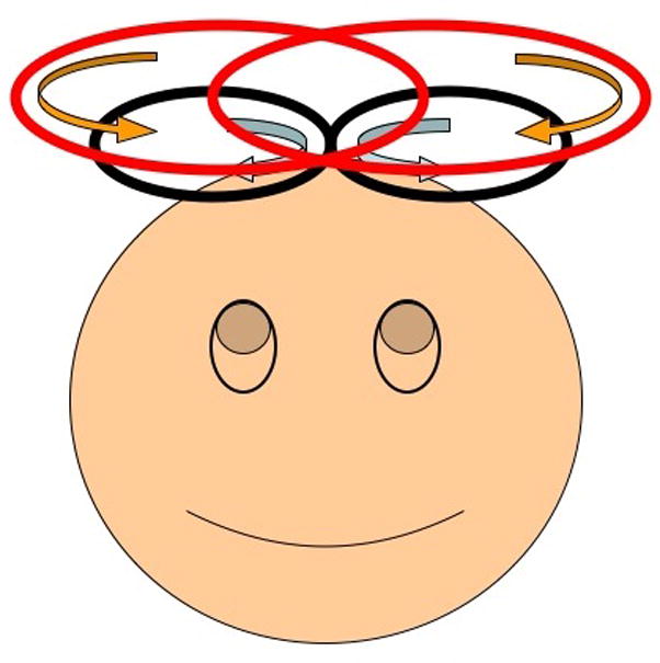
Shielding coil (red) used in conjunction with a figure-eight TMS coil (black). The parameters to be optimized were the main current to be applied to the opposing coil, the size and the vertical position of the shielding coil The parameters to be optimized were the main current to be applied to the opposing coil, the radius and the vertical position of the shielding coil.

Figure 2.

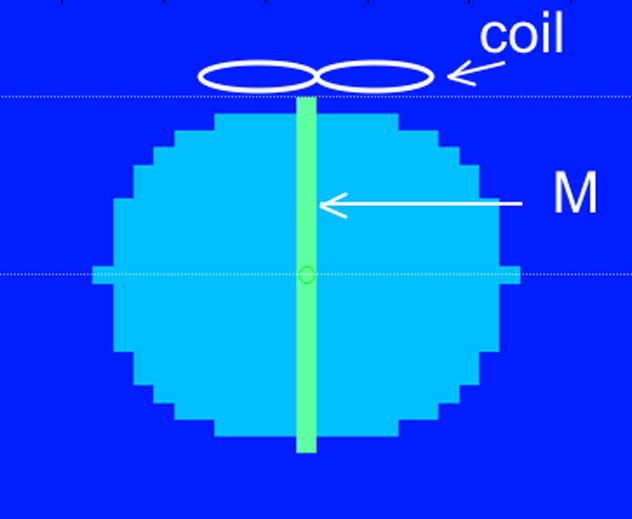
The coarse sphere and cylinder used for the optimization process. The sphere’s diameter is 15 cm. The figure-eight coil was 1 cm above the sphere. The diameter of each loop was 6 cm. “Sharpness” (S) was defined as the ratio of the integral of the electric field’s magnitude inside the cylinder to the integral of the electric field’s magnitude over the whole sphere. “Penetration” (P) was defined as the ratio of the magnitude of the electric field at the midpoint (M) between the sphere’s surface and center to its magnitude on the surface (3.75 cm deep).

$$\mathit{C}(\mathit{W})=\underset{\{\mathit{z},\mathit{R},\mathit{F}\}}{min}\left|\frac{1}{\mathit{S}(\mathit{z},\mathit{R},\mathit{F})}+\frac{\mathit{W}}{\mathit{P}(\mathit{z},\mathit{R},\mathit{F})}\right|$$ (2)

where z, R and F are the design parameters to be optimized: distance, size and current fraction. This cost function incorporates a parameter (W) that weighs the relative importance placed on each of the objectives. To calculate the cost function we approximate each individual closed coil current source by 10 piecewise linear elements and apply a midpoint quadrature rule to calculate the electric field using eqn.1.

Optimizations were performed using values of W from 0 to 12 in order to investigate a range of designs optimized for sharpness and/or penetration. The shield design parameters (z,R,F) were optimized by an iterative trust-region-reflective algorithm. This algorithm searches for the minimum of a cost function in eqn.1, subject to a set of user-specified constraints which in our case were the prescribed ranges of the various shield parameters.

For each of the 12 final shield designs we compute other electric field parameters by sampling the field inside the spherical region on cubic Cartesian grid with edge length of 1.875 cm. We define the “activated region”, as in Thielsher and Kammer, as the region of the sphere which has an electric field magnitude that is at least 50% that of the maximum field on the sphere (Thielscher and Kammer, 2004). From this measure of we define the “penetration depth” as the vertical distance from the top of the sphere to the lowest active point on the sphere, and the “activation area” as the area on the sphere’s surface above threshold.

In order to achieve a practical time to convergence, the minimization of the cost function was carried out on a coarse grid (33 × 33 × 33) covering a volume of 24 × 24 × 24 cm. On this coarse implementation, the line segments on the wire loop (dl) were generated by sampling ten equidistant locations on each loop of the coil. Upon convergence of the algorithm, the resulting active shields were used to re-calculate the electric field produced by a standard figure-eight coil in conjunction with each field on a finer grid (128 × 128 × 128). Note that the spatial frequency content of these fields is quite low (i.e., the fields are smooth) and thus the minimum on the cost function at a coarse resolution should be very close to the minimum at a higher resolution.

Although the optimizations were conducted assuming the coils were excited in isolation/free-space, we also tested their validity in the presence of a realistic model of a human head. Conductivity maps were constructed by segmenting a high resolution MRI image. The image was obtained by scanning a single male subject in a 3T GE Signa scanner (Waukesha, WI) using an IR-prepped, 3D, SPGR pulse sequence (TR=9.03, TE = 1.84, TI = 500 ms. Matrix size = 256 × 256 × 124, FOV = 24 cm, slice thickness = 1.2 mm). The first step in segmentation was the identification of gray mater, white mater, and ventricular CSF by the SPM5’s segmentation toolbox (http://www.fil.ion.ucl.ac.uk/spm). The remaining unclassified tissue was further partitioned into another three types (bone, muscle, CSF) by FAST (part of the FSL’s image analysis package http://www.fmrib.ox.ac.uk/fsl/). Conductivities were assigned to each tissue type using values obtained from the literature (Salinas et al., 2009). The resulting conductivity maps were sub-sampled to a cubic matrix of 1283 voxels prior to calculating the electric fields.

To analyze buildup of charges on different conductive interfaces between tissue types we a implemented the quasi-static finite difference method proposed by Cerri et al (Cerri et al., 1995). In this method displacement currents are neglected, as they are much smaller than conduction currents. The same holds true for magnetic fields scattered by the human head as they are small relative to the magnetic field produced by the coil. Within these assumptions the Cerri method allows one to compute the electric field vector component on each edge internal to a Cartesian mesh made up of piecewise homogenous cubic conductive elements. All simulations and optimizations were performed using custom Matlab (The Mathworks, South Nattick, MA) scripts, running on a personal computer.

Results

Figure 3 shows the percentage change in the penetration and sharpness of each shielded coil design relative to the coil alone for each of the 12 different shielded coil designs. It appears that in all cases one can increase penetration or increase sharpness but not both. We do note that if one is willing to sacrifice 16,67% of the penetration depth (0.19 cm), one can reduce the excited area on the surface by 34.24% and the excited volume by 43.87 %, as in the case of the optimization with W=3; we will call this design “W30 shield” from now on. Please note that depending on the desired stimulation region, other designs may be more appropriate and in that spirit we have listed the various parameters extracted with different cost functions.

Figure 3.

Change in sharpness and penetration upon convergence of the optimization algorithm as a function of the penetration weight parameter (W). The plot indicates the trade-off between the two quantities.

Table 1 shows the optimal shield design parameters, the sharpness and penetration, and information about the “activated region” for each of the 12 optimizations. Furthermore, the table indicates the same shape parameters calculated after scaling the electric field magnitude such that the penetration depth is preserved for each probe design. The scaled Activation Shape information shows that if we were to increase the the penetration depth by turning up the power until the same penetration depth is achieved (1.13 cm), then the shield still reduces the activated surface area of the sphere by 10.34% and the total activated volume by 13.32%.

Table 1.

Weight Parameter	(no shield)	0.00	2.00	3.00	4.00	6.00	8.00	10.00	12.00
Optimized Field features:
Sharpness Increase (%)		61.41	57.73	46.37	30.71	16.65	12.17	4.02	−17.09
Penetration Increase (%)		−51.61	−46.05	−38.27	−26.06	−11.63	−8.11	−2.71	27.98
Shield Parameters:
Shield Current (%)		−78.26	−75.27	−77.68	−135.39	−24.91	−17.53	−5.95	300.00
Shield Radius (cm)		3.50	3.50	3.50	3.50	12.00	12.00	12.00	3.89
Shield Position (cm)		9.00	9.00	9.48	13.13	25.00	25.00	25.00	9.00
Activation Shape
Deepest activation (cm)	1.13	0.75	0.75	0.94	0.94	1.13	1.13	1.13	1.31
Active Surface (cm2)	14.27	8.30	8.44	9.39	11.85	13.25	13.25	14.13	18.67
Active Volume (cm3)	9.30	4.33	4.42	5.22	6.80	8.27	8.54	9.10	14.23
Max. Field (at scalp)	1.00	1.00	1.00	1.00	1.00	1.00	1.00	1.00	1.00
Deepest activation (% change)		−33.33	−33.33	−16.67	−16.67	0.00	0.00	0.00	16.67
Active Surface (% change)		−41.87	−40.89	−34.24	−17.00	−7.14	−7.14	−0.99	30.79
Active Volume (% change)		−53.44	−52.45	−43.87	−26.86	−11.13	−8.15	−2.20	53.01
Max. Field at scalp (% change)		0.00	0.00	0.00	0.00	0.00	0.00	0.00	0.00
Activation Shape (scaled for depth)
Deepest activation (cm)		1.13	1.13	1.13	1.13	1.13	1.13	1.13	1.13
Active Surface (cm2)		12.45	12.48	12.80	13.01	14.27	14.24	14.27	15.33
Active Volume (cm3)		7.73	7.84	8.06	8.44	9.20	9.20	9.30	10.36
Max. Field (at scalp)		1.22	1.19	1.15	1.08	1.02	1.02	1.01	0.91
Deepest activation (% change)		0.00	0.00	0.00	0.00	0.00	0.00	0.00	0.00
Active Surface (% change)		−12.81	−12.56	−10.34	−8.87	0.00	−0.25	0.00	7.39
Active Volume (% change)		−16.87	−15.66	−13.32	−9.21	−1.06	−1.13	0.00	11.41
Max. Field (at scalp) (% change)		21.71	18.92	14.87	8.10	2.49	1.72	0.57	−8.75

We believe that the shielded W30 design delivers a much more compact pulse at the cost of a little penetration. Figure 4 contains orthogonal views of the magnitude of the electric field magnitude calculated without shielding (panel A) and with the W30 shield design (panels B and C). Images in panels A and B are normalized such that the maximum electric field magnitude on the surface is the same in all cases. The normalized fields are shown on a dB scale to facilitate visualization of the large range of values. One can observe how the shield contains the unwanted electric fields, shaping the stimulated region into a narrower, more focal one at the cost of depth penetration. Panel C is scaled such that the penetration depth of the unshielded coil is restored. In this case, the entire field is scaled such that the penetration depth of the shielded case is matched to the unshielded case. In this case, however, the maximum electrical field magnitude at the surface of the sphere is 14.87% higher. Profile plots of the same data are shown in figure 5. These plots were extracted from the center of the field of view along the x and y axes, and at 1.13 cm below the surface of the sphere directly below the coil.

Figure 4.

High resolution, orthogonal views of the magnitude of the electric field calculated without shielding (A), with the W40 shield (B) and with the W30 shield while adjusting the power to restore the original penetration depth. The position of the coil in each plane is indicated by the white ellipses (not to scale). The images are shown on a 20*log scale to facilitate visualization of the large span of values. The three orthogonal views intersect at the center of the horizontal slice 1.13 cm below the surface of the sphere (the location of the deepest activation produced by the unshielded coil). These images are scaled such that the maximum electric field magnitude on the surface is the same in panels A and B. The field in panel C has been scaled such that its field at 1.13 cm deep below the surface under the coil matches that of the unshielded case (panel A). The shield reduces the activated region’s volume and surface, but also reduces the penetration depth. Penetration depth can be recovered by increasing the power to the system and the volume and surface of the activated region are still less than in the unshielded case. However, the maximum field on the surface increases in that case. The tick marks on the images indicate pixels.

Figure 5.

Profile plots of the electric field at the center of the field of view along the x and y axes, and 1.13 cm under the center of the coil along the z axis. The electric field is also plotted on a 20*log scale in order to display the large range of values in the field.

Figure 6 contains the calculated magnitude of the electric fields inside the brain for the W30 shielded and the unshielded design. Figure 7 shows the axis profiles through a point in the middle of the slice 1.28 cm below the surface of the skin. The reduction in penetration and the containment of the main field by the active shield can be seen from the figures. Simulations on human head conductivity models, taking the contribution from surface charges, yielded a reduction of penetration depth of 16.6% (from the original 1.28 cm) due to the W30 shield. The activated volume was reduced by 24.1%. If we scale the field so that the penetration depth is restored to 1.28 cm, the activated volume actually increases by 2.9% but the volume is still reduced by 13.1% relative to the unshielded case. Scaling up the field to restore penetration depth causes the maximum electric field at the scalp to be 16.3% greater than in the unshielded case.

Figure 6.

Magnitude of the electric field induced by an unshielded TMS coil (panel A) and a shielded one (panel B). Panel C shows the same field as in B, but scaled such that the penetration depth is restored. Fields were calculated taking into account the effects of surface charges.

Figure 7.

Profile plots along the principal axes of the electric field generated in a brain. The intersection point is sampled at the center of the xy plane and at 1.28 cm below the surface of the scalp, directly below the middle of the coil. The tick marks on the images indicate pixels. The images are shown on a 20*log scale to facilitate visualization of the large span of values.

Discussion and Conclusions

In this article we have presented a new strategy to design TMS probes with greater focality. The strategy consists of shielding the TMS probe actively with a secondary probe, whose fields cancel the electric fields outside the desired target. Analytical optimization of these designs can be difficult, so we have taken a numerical approach to optimize the design parameters. The measures of goodness for our optimization were the sharpness and the penetration of the electric field within a target sphere simulating a human head. It is important to note that, for our purposes, the specific design of the primary coil (a figure-eight coil in our case) is not the focus of this article, since the strategy that we present can be applied to most coils. It is not the aim of this paper to design the best possible coil, but to introduce a design strategy for future designs.

In order to gain an intuition of the effects of the radius, position and current of the shield individually on the sharpness and penetration parameters, figure 8 shows the sharpness and penetration for a range of shield parameters (Unless otherwise specified, the default shield parameters are were: current factor = −0.7, radius = 4 cm, shield position = 9.5 cm, or 2 cm above the head). The trade-off between penetration and sharpness is evident. There are no clear maxima in this 3D search space.

Figure 8.

Sharpness and Penetration as a function of the shield design parameters. Unless otherwise specified, the relative current, radius, and vertical position were held constant at −0.7, 4.0 cm, and 9.5 cm. Note that Sharpness and Penetration are ratios and therefore have no units. Also note, that in these plots, Sharpness is multiplied by 10 for scaling purposes.

We note that TMS coils have been characterized by the supra-threshold area on the surface (Thielscher and Kammer, 2004) as a measure of goodness. While we report those parameters in our final design, we chose different criteria for the cost function for three reasons. First, the coarse grid used to simulate the fields in our algorithm caused the minimization to converge at local minima when using supra-threshold areas. Secondly, we are interested in reducing extraneous fields even if they are subthreshold because geometric variability due to positioning of the coil, or to the subjects’ anatomy can potentially lead to unwanted activation in near-threshold regions because of additional fields created by charge build-up.

It is well-known that the buildup of surface charges along the interfaces between tissue types create additional electric fields that distort the shape of the net electric field. However, our approach was to optimize only the incident field created by the TMS coil for two reasons. First, given actual computational speed, our iterative design algorithm would be quite impractical if surface charges were to be considered (a single calculation takes approximately four hours). More importantly, perhaps, given that TMS probes are used over multiple locations on the brain, a probe that has been designed optimally for for a specific sulcus in a specific subject is likely to be sub-optimal in other regions, or other subjects. Thus, we chose to optimize the designs based on the primary incident electric in order to design a versatile system, as in previous efforts (Pu et al., 2008; Roth et al., 2007; Thielscher and Kammer, 2004; Tofts, 1990). At that point, we verified that the new coil was still advantageous in a more realistic model, i.e., computing the electric fields including the effects of the charge buildup at tissue boundaries. There may be situations in which it is desirable to design a stimulation coil for a specific subject’s head, we have taken an approach of designing a general case TMS coil. In that case, the same iterative optimization techniques presented here can still be applied, but the computational time will be in the order of several days, as mentioned. Furthermore, in most cases, improving the focality of primary incident fields in free space should translate into more focal total fields when the surface charges are taken into consideration, as these surface charges typically have a distorting effect on the primary field. The simulations presented of human head conductivity models presented above seem to corroborate this claim, at least for the selected coil orientation and position, where the changes in focality and depth penetration due to the active shield in free space translated into comparable changes in the realistic head model.

We have shown that there is a trade-off between the sharpness and penetration of the coil depending on how much weight each of these is given in the cost function. It is interesting to note that when penetration depth is lost by a specific design, it can be recovered by increasing the current to the system at the expense of some of the gain in sharpness. A second price to pay is the increased electric field on the surface. While this can lead to greater discomfort to the subject, it may not necessarily affect the neurological effects. This is then a matter for the researcher/clinician to decide what parameter is more important. Often, as in the case of motor stimulation, the target tissue is close enough to the surface that giving up half a centimeter may not be detrimental for the experiment.

A foreseeable caveat of active shields is the induction of Lorentz forces between the primary and the shielding coils. As a quick approximation, we can use Ampere’s force law to calculate the force between two concentric loops of 3 and 3.5 cm radius, carrying 1 kA and −1.3 kA respectively. This results in an attractive force of 215 Newtons. This force will be applied briefly (less than 1 msec) on the coil and will produce mechanical stress and vibration on the system. Hence, construction of such probes will require mechanical reinforcement and vibration damping to prevent damage to the subject and the equipment.

References

- Burt T, Lisanby S, Sackeim H. Neuropsychiatric applications of transcranial magnetic stimulation: a meta analysis. Int J Neuropsychopharmacol. 2002;5:73–103. doi: 10.1017/S1461145702002791. [DOI] [PubMed] [Google Scholar]
- Cerri G, De Leo R, Moglie F, Schiavoni A. An accurate 3-D model for magnetic stimulation of the brain cortex. J Med Eng Technol. 1995;19:7–16. doi: 10.3109/03091909509030264. [DOI] [PubMed] [Google Scholar]
- Davey KR, Riehl M. Suppressing the surface field during transcranial magnetic stimulation. IEEE transactions on bio-medical engineering. 2006;53:190–194. doi: 10.1109/TBME.2005.862545. [DOI] [PubMed] [Google Scholar]
- Edelstein W, Kidane T, Taracila V, Baig T, Eagan T, Cheng Y, Brown R, Mallick J. Active-passive gradient shielding for MRI acoustic noise reduction. Magn Reson Med. 2005;53:1013–1017. doi: 10.1002/mrm.20472. [DOI] [PubMed] [Google Scholar]
- Ellison A, Cowey A. Time course of the involvement of the ventral and dorsal visual processing streams in a visuospatial task. Neuropsychologia. 2007 doi: 10.1016/j.neuropsychologia.2007.06.014. [DOI] [PubMed] [Google Scholar]
- George MS, Belmaker RH. Transcranial magnetic stimulation in neuropsychiatry. 1. American Psychiatric Press; Washington, DC: 2000. [Google Scholar]
- Jalinous R. Technical and practical aspects of magnetic nerve stimulation. J Clin Neurophysiol. 1991;8:10–25. doi: 10.1097/00004691-199101000-00004. [DOI] [PubMed] [Google Scholar]
- Kahkonen S, Ilmoniemi R. Transcranial magnetic stimulation: applications for neuropsychopharmacology. J Psychopharmacol. 2004;18:257–261. doi: 10.1177/0269881104042631. [DOI] [PubMed] [Google Scholar]
- Levit-Binnun N, Handzy N, Moses E, Modai I, Peled A. Transcranial Magnetic Stimulation at M1 disrupts cognitive networks in schizophrenia. Schizophr Res. 2007;93:334–344. doi: 10.1016/j.schres.2007.02.019. [DOI] [PubMed] [Google Scholar]
- Li X, Nahas Z, Anderson B, Kozel F, George M. Can left prefrontal rTMS be used as a maintenance treatment for bipolar depression? Depress Anxiety. 2004;20:98–100. doi: 10.1002/da.20027. [DOI] [PubMed] [Google Scholar]
- Lisanby S, Kinnunen L, Crupain M. Applications of TMS to therapy in psychiatry. J Clin Neurophysiol. 2002;19:344–360. doi: 10.1097/00004691-200208000-00007. [DOI] [PubMed] [Google Scholar]
- Lu M, Ueno S. Calculating the electric field in real human head by transcranial magnetic stimulation with shield plate. PROCEEDINGS OF THE 53RD ANNUAL CONFERENCE ON MAGNETISM AND MAGNETIC MATERIALS; Austin, Texas (USA): AIP; 2009. pp. 07B322–323. [Google Scholar]
- Mansfield P, Chapman B. Active magnetic screening of coils for static and time-dependent magnetic field generation in NMR imaging. J Phys E: Sci Instrum. 1986;19:540–545. [Google Scholar]
- Paige CC, Saunders MA. LSQR: An Algorithm for Sparse Linear Equations and Sparse Least Squares. ACM Trans Math Softw. 1982;8:43–71. [Google Scholar]
- Pascual-Leone A, Walsh V, Rothwell J. Transcranial magnetic stimulation in cognitive neuroscience--virtual lesion, chronometry, and functional connectivity. Curr Opin Neurobiol. 2000;10:232–237. doi: 10.1016/s0959-4388(00)00081-7. [DOI] [PubMed] [Google Scholar]
- Pitcher D, Walsh V, Yovel G, Duchaine B. TMS Evidence for the Involvement of the Right Occipital Face Area in Early Face Processing. Curr Biol. 2007;17:1568–1573. doi: 10.1016/j.cub.2007.07.063. [DOI] [PubMed] [Google Scholar]
- Pu L, Yin T, An H, Li S, Liu Z. Optimization of the Coil to Focalize the Electrical Field Induced by Magnetic Stimulation in the Human Brain. 7th Asian-Pacific Conference on Medical and Biological Engineering; 2008. pp. 366–372. [Google Scholar]
- Roth Y, Amir A, Levkovitz Y, Zangen A. Three-dimensional distribution of the electric field induced in the brain by transcranial magnetic stimulation using figure-8 and deep H-coils. J Clin Neurophysiol. 2007;24:31–38. doi: 10.1097/WNP.0b013e31802fa393. [DOI] [PubMed] [Google Scholar]
- Roth Y, Zangen A, Hallett M. A coil design for transcranial magnetic stimulation of deep brain regions. J Clin Neurophysiol. 2002;19:361–370. doi: 10.1097/00004691-200208000-00008. [DOI] [PubMed] [Google Scholar]
- Rothwell J. Paired-pulse investigations of short-latency intracortical facilitation using TMS in humans. Electroencephalogr Clin Neurophysiol Suppl. 1999;51:113–119. [PubMed] [Google Scholar]
- Salinas FS, Lancaster JL, Fox PT. 3D modeling of the total electric field induced by transcranial magnetic stimulation using the boundary element method. Physics in Medicine and Biology. 2009:3631–3647. doi: 10.1088/0031-9155/54/12/002. [DOI] [PMC free article] [PubMed] [Google Scholar]
- Thielscher A, Kammer T. Electric field properties of two commercial figure-8 coils in TMS: calculation of focality and efficiency. Clinical neurophysiology: official journal of the International Federation of Clinical Neurophysiology. 2004;115:1697–1708. doi: 10.1016/j.clinph.2004.02.019. [DOI] [PubMed] [Google Scholar]
- Tofts PS. The distribution of induced currents in magnetic stimulation of the nervous system. Physics in Medicine and Biology. 1990:1119–1128. doi: 10.1088/0031-9155/35/8/008. [DOI] [PubMed] [Google Scholar]
- Turner R. Gradient coil design: a review of methods. Magn Reson Imaging. 1993;11:903–920. doi: 10.1016/0730-725x(93)90209-v. [DOI] [PubMed] [Google Scholar]