A new approach to estimating the signal dimension of concatenated resting-state functional MRI data sets

Abstract

Estimating the effective signal dimension of resting-state functional MRI (fMRI) data sets (i.e., selecting an appropriate number of signal components) is essential for data-driven analysis. However, current methods are prone to overestimate the dimensions, especially for concatenated group data sets. This work aims to develop improved dimension estimation methods for group fMRI data generated by data reduction and grouping procedure at multiple levels. We proposed a “noise-blurring” approach to suppress intragroup signal variations and to correct spectral alterations caused by the data reduction, which should be responsible for the group dimension overestimation. This technique was evaluated on both simulated group data sets and in vivo resting-state fMRI data sets acquired from 14 normal human subjects during five different scan sessions. Reduction and grouping procedures were repeated at three levels in either “scan–session–subject” or “scan–subject–session” order. Compared with traditional estimation methods, our approach exhibits a stronger immunity against intragroup signal variation, less sensitivity to group size and a better agreement on the dimensions at the third level between the two grouping orders.

1. Introduction

Data-driven analysis methods, such as principal component analysis (PCA) [1] and independent component analysis (ICA) [2], have been shown to be promising tools for detecting cerebral activity and/or connectivity in functional MRI (fMRI) without a priori knowledge. This is particularly true for resting-state fMRI analysis [3,4] because of its ability to investigate exploratively in the absence of regional hypothesis, as required for seed-based analysis [5]. Nevertheless, a theoretical and practical barrier to current data-driven analysis is estimation of signal dimension (i.e., choosing an appropriate number of signal components in data-driven analysis) [6]. Previous studies have indicated that using different numbers of signal components may have significant impacts on PCA or ICA decomposition results [1,7]. More specifically, underestimation of the signal dimension may introduce a mixture of distinct functional network components, whereas overestimation would break down a single functional network into multiple components of unrecognizable fractures [7].

In many applications, a number of individual fMRI data sets are usually concatenated in time domain to construct a group data set and to perform data-driven analysis on the group to obtain more robust or populationwise results [6]. Thus, for data reduction, the estimation of signal dimension has become necessary at both individual and group levels in order to reduce data size without losing effective information [8,9]. It has been noted that if we simply apply data-driven algorithms on each individual data set and then perform group analysis on decomposed data space, one may have to deal with the difficulties of finding and quantifying the matched components across the data sets within the group [10].

Traditionally, the signal dimension of fMRI data could be evaluated by applying classic stochastic signal modeling techniques such as the Akaike information criterion (AIC) [11], Bayesian information criterion (BIC) [12] and minimum description length (MDL) [13]. The legibility of doing so was based on fMRI data possessing the properties that fully comply with the assumption underlying these traditional signal and noise models, such as the white-noise spectrum assumption about noise [14]. Nevertheless, previous studies have shown that the traditional techniques tend to substantially overestimate the signal dimension of resting-state fMRI data, even in the simplest case of an individual data set [8,15].

For group fMRI data, dimension overestimation can be severer in traditional methods because the data reduction and concatenation procedures may force the spectral properties of the group data to be further biased from the original signal and noise assumptions [16]. This problem may worsen in the case of data reduction performed at multiple grouping levels due to the cumulating effects of spectral bias. In practice, the difficulty of dimension overestimation is highlighted by a proportional increase in estimated signal fMRI dimensions with respect to group size [17]. Consequently, traditional methods are prone to report an unreasonably high dimension for group fMRI data, usually equal to or approximating the total number of data points in the time domain [2,8,15]. This problem may lead to an inability to incorporate data-driven analyses for varying group sizes, as well as to difficulty with sufficient data reduction, which usually means that a gigantic volume of fMRI data cannot be processed in a regular computer system for a large group.

It has been demonstrated that the autoregressive structure of fMRI data, which is biased from the white-noise assumption underlying traditional methods, is responsible for dimension overestimation at the individual acquisition level [15,18]. Cordes and Nandy [15] proposed an alternative strategy to estimate the signal dimension of fMRI data under the assumption of autoregressive noise. The core procedure was to use a first-order autoregressive (AR(1)) model to fit the noise structure into the PCA eigenvalue spectrum and then to use the divergent point between the fitted noise spectrum and the actual signal spectrum as an indicator of effective signal dimension [15]. The authors showed that this method could significantly reduce the dimension overestimation for individual fMRI data sets. Like other existing techniques, however, this AR(1) fitting method has not been evaluated for concatenated group fMRI data sets, where the effects of data reduction may be involved. As mentioned above, a dimension estimation method that is valid for individual data sets is not necessarily valid for group-level data sets because of intragroup signal variations and spectral alterations caused by the data reduction procedure.

To address these difficulties, we present a study that aims to develop a new method for estimating signal dimensions for group fMRI data generated by reduction and grouping at multiple levels. In vivo fMRI data sets were acquired to investigate dimension behaviors at individual scan, cross-subject (or session) and third “grand” levels. A “noise-blurring” technique was developed to suppress intragroup signal variations and to correct spectral alterations by adding artificially generated autoregressive noise to the group data. We specified the properties of blurring noise based on the assumption that the postnoise group data set should have a PCA spectrum similar to the average PCA spectrum of the original subgroup fMRI data sets prior to the data reduction. Our results suggested that the proposed “noise-blurring” technique could be applied to various dimension estimation methods, whereas the best performance was obtained by employing the (AR(1)) noise-fitting technique [15] to estimate the signal dimension of the group fMRI data. In comparison with traditional methods, our approach exhibited a stronger immunity against intragroup signal variation, less sensitivity to group size and a better agreement on the dimensionality at the third level between the two grouping orders.

2. Methods

2.1. Data acquisition and preprocessing

Fourteen (N=14) healthy volunteers (30±6 years old, all male and right-handed) were scanned in resting state for five sessions (M=5) on a 3-T Siemens Allegra (Siemens, Erlangen, Germany) scanner on five different days over a period of 14 days. Written informed consent was obtained from each subject in accordance with the guidelines of the Institutional Reviewer Board at the National Institute on Drug Abuse. A gradient-echo echoplanar imaging (EPI) pulse sequence was used to acquire whole-brain resting-state fMRI images, including 39 sagittal 4-mm-thick slices. Echo time (T_E) and repetition time (T_R) were set to 27 and 2160 ms, respectively. The field of view of the image was 22×22 cm², with an in-plane matrix size of 64×64. For each resting-state scan, 86 repetitions were acquired over 3.1 min. Subjects were instructed to keep their head still, to close their eyes and to not think of anything in particular. Ear plugs were used to reduce acoustic noise, and foam packs were applied to restrict head motion. T₁-weighted anatomical images were also acquired for spatial normalization. Due to scanner failure, data on one subject were lost for Session 1, data on one subject were lost for Sessions 2 and 3, and data on one subject were lost for Session 5. Missing data are properly excluded from the image processing procedure, as described below.

All resting-state EPI data sets were volume-registered in the time domain to correct for subject head motion and sinc-interpolated to correct for slice–timing effects. Based on the corresponding T₁-weighted high-resolution images, the EPI data were then spatially normalized to Talairach space [19], spatially smoothed with a Gaussian kernel with a full width at half maximum of 4 mm and resampled to 3×3×3 mm³. The data were preprocessed with AFNI [20]. No masking procedure was involved in the processing in order to keep the image background, which provides useful information on noise structures.

2.2. PCA spectrum and AR(1) fitting

For each preprocessed four-dimensional (4D) spatiotemporal data set, a PCA algorithm [1] was applied with respect to the spatial domain to calculate the eigenvalue spectrum (i.e., the descending-ordered PCA eigenvalues of the data). The PCA spectrum had an identical length as the total time points of the data set, where the larger eigenvalues (in the spectral head) and the smaller eigenvalues (in the spectral tail) were assumed to characterize contributions from signal and noise components in the fMRI data, respectively. Thus, the estimation of signal dimension was equivalent to finding an appropriate divergent point between the signal section and the noise section of the PCA spectral curve. If a white-noise spectrum were assumed, a dimension overestimation would occur because a shorter noise section would be identified based on the fact that white noise should have a “flat” tail in the PCA spectrum [15]. To avoid this problem, we implemented an AR(1) modeling technique to fit the colored noise structure of the PCA spectrum, as previously described by Cordes and Nandy [15]. Due to the improved capability of AR(1) model to capture a colored noise tail, the observed divergent point between signal and noise sections would move towards the spectral head, leading to a decreased estimation of the signal dimension. In this study, the eigenvalues in the lower 30% [21,22] of the spectral tail (excluding the least 20 eigenvalues [15]) were assumed to be pure noise components and thus were taken into the AR(1) fitting. The signal/noise divergent point was identified as the place where the fitted and actual spectra crossed each other and then diverged to a distance greater than 0.1% of the largest eigenvalue; thus, the index of the divergent point in the PCA spectrum was used to represent the signal dimension of the fMRI data. For comparison, the traditional techniques for dimension estimation (AIC, BIC and MDL) were also performed in accordance with Akaike [11], Weakliem [12] and Rissanen [13].

2.3. Data reduction at multiple levels

Let D_ij (where i=1, 2, …, M; j=1, 2, …, N) be an arbitrary individual fMRI data set acquired from subject j at session i. Data reduction for D_ij was conducted by reconstructing the fMRI data $D_{ij}^{\prime }$ from the denoised PCA spectrum, where the noise components of D_ij were removed [18] based on the estimated signal dimension Dim(D_ij), as described above. Group data were produced by concatenating the multiple postreduction 4D fMRI data sets along the time direction, and then dimension estimation and data reduction were applied again to the group data. As illustrated in Fig. 1, this “reduction and grouping” procedure could be repeated at multiple group levels with different grouping orders. (1) For “scan–subject–session” order, first-level reduction was applied to each individual scan data set D_ij; second-level reduction was then applied to five groups (Sess_i*, where i=1, 2, …, M) comprising all processed individual data across 14 subjects; and, finally, third-level reduction was applied to the “grand” group comprising the five post-reduction second-level data sets ( ${\text{Sess}}_{i\ast }^{\prime }$, where i=1, 2, …, M) across all sessions. (2) For the “scan–session–subject” order, first-level data reduction was the same as that of the above; the 14 groups (Subj_*j, where j=1, 2, …, N) across all sessions were processed at the second level; and the “grand” group comprising all 14 postreduction groups ( ${\text{Subj}}_{\ast i}^{\prime }$, where j=1, 2, …, N) was processed at the third level. See Fig 1 for an example of reduction for the “scan–subject–session” order.

Fig. 1.

Multiple level data processing diagram for fMRI dataset dimension estimation (DE), data reduction, and grouping, illustrated with the order of “scan-subject-session”. Dij and D′ij denote the original and postreduction individual fMRI dataset acquired from subject j at session i, respectively. Sessi and Sess′j are the pre- and postreduction group data for session j across all subjects. Dimensional estimation at level 1 (DE1) is applied to all individual datasets, whereas DE2 and DE3 are performed for the group datasets by adding blurring noise whose parameters are determined by minimize the sum of square error (SSE) of the PCA spectral difference between the postnoise group datasets and the prereduction subgroup datasets.

2.4. Noise-blurring technique

Let G be an arbitrary group data set comprising subgroup data sets $D_i^{\prime }$ (i=1, 2, …, N), which were generated by data reduction from the original data sets D_i (i=1, 2, …, N). In general, the PCA eigenvalue spectrum of group G, denoted by S(G), would decay more slowly than the spectra of the original data sets S(D_i) due to signal variations among the subgroup data sets that caused fluctuation and reordering of the signal eigenvalues in S(G)), leading to a significant overestimation for Dim(G) (see Results for an example). On the other hand, the data reduction process also altered the subgroup spectra $S(D_i^{\prime })$ by removing the noise components from S(D_i) according to the estimated Dim(D_i). Thus, the traditional dimension methods might not be valid for group G even though they could work perfectly with the individual data sets D_i.

We proposed an approach to suppressing intragroup signal variances and reduction-introduced spectral alterations by adding artificial autoregressive noise to the group data set G prior to dimension estimation. This blurring noise, denoted by n(φ), was generated by a Gaussian AR(1) series with an autoregressive coefficient (φ) that was set as the average φ value fitted from all original subgroup data sets D_i (i=1, 2, …, N) in accordance with Cordes and Nandy [15]. The strength of the blurring effect was controlled by the noise ratio (nr), defined as the ratio of the standard deviation of the blurring noise to the standard deviation of the group data. The postnoise group data set can be written as G_nr=G+nr*n(φ), and the optimal nr was determined by minimizing the sum of square error (SSE) Δ(nr) between the sum PCA spectrum of all prereduction subgroup data sets D_i (i=1, 2, …, N) and the PCA spectrum of the postnoise group data set G_nr, such that $\mathrm{\Delta }(\text{nr})={\displaystyle \sum _{k=1}^L}{\left\{S(G_{\text{nr}})-{\displaystyle \sum _{i=1}^N}S(D_i)\right\}}_k^2\stackrel{nr}{\to }\mathit{min}$, where descending-ordered eigenvalues k=1~L in the PCA spectra were used to estimate the optimal nr.

This noise-blurring technique for group dimension estimation was based on the assumption that the postnoise group data G_nr should have a spectral structure as close as possible to that of the original prereduction subgroup data sets, so that the spectral alterations introduced by the data reduction and grouping procedures can be corrected. Thus, regular dimension methods, assuming they were able to work properly with original data sets, can be expected to provide comparable results for the postnoise group data under a similar spectral condition. It should be noted that the postnoise group G_nr was only used for the purpose of dimension estimation, whereas the actual procedures of data reduction and grouping were performed on the prenoise data sets D_i (i=1, 2, …, N).

2.5. Computer simulations

To provide an additional assessment to the proposed dimension estimation procedure, we also performed an analysis on computer-generated data sets, processed similarly to that described above. In each simulated individual data set, a mixture of random Gaussian white noise and 16 non-Gaussian independent signal sources (components), with a spatial size of 120×120 at 200 time points, was generated (see supplementary file doi:10.1016/j.mri.2010.04.002). Similar to the in vivo case, 14 “subjects” (or “sessions”) of simulated data sets were generated. By following the same procedures as depicted in Fig. 1, we performed the dimension estimation, reduction and grouping steps on the simulated data sets.

In the case of zero signal variation, the 16 signal sources were assumed to be identical across all subgroup data sets to create a known signal dimension of 16 for the group data. When intragroup signal variations needed to be taken into account, random white Gaussian fluctuations were added to the 16 sources to create signal variations among the subgroup data sets. Thus, the effective group dimension could be characterized with respect to the signal variation strength, which was quantified by the standard deviation ratio between the added random fluctuations and the 16 signal sources. Noted that this “adding signal variation” procedure differs in nature from “blurring noise” in terms of dimensionality estimation because we employed a “white” spectral signal variation (i.e., the fluctuations series were independent in each time point) to avoid introducing autoregression changes in the group data.

3. Results

3.1. Individual data sets

Fig. 2 illustrates the PCA eigenvalue spectra of the five individual fMRI data sets acquired from the five sessions of a typical subject, with observable variation among the sessions. The averaged PCA spectrum is used to demonstrate the dimension estimation based on the AR(1) fitting technique. The descending-sorted eigenvalues located within the fitting range (35–65) are used to generate the fitted noise spectrum. The divergent point between this fitted noise spectrum and the averaged signal spectrum curves indicates a signal dimension of 30 in this example. Applying this AR (1) fitting technique to each individual data set for this subject, we obtain dimensionalities of 28, 26, 28, 33 and 30, respectively, from Sessions 1 through 5. The average goodness of fit for these five individual data sets is 0.93±0.03. In general, a data set where the eigenvalues decay more slowly in the PCA spectrum would tend to give a larger dimension estimation and vice versa.

Fig. 2.

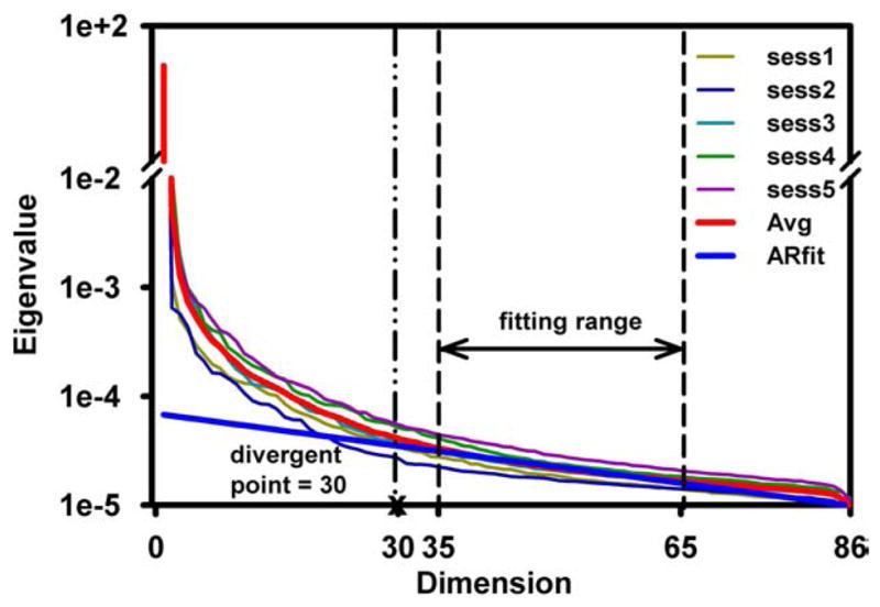
Five 1st level individual fMRI datasets acquired from five scan sessions of one subject are used to generate the PCA eigenvalue spectra, depicted as five thin colored curves, with apparent variations behave among them. The averaged PCA spectrum (bold red curve) is used to demonstrate the dimensional estimation based upon the AR(1) fitting technique. The eigenvalues located within the fitting range (33–65) are used to generate the fitted noise spectrum (solid blue line). The divergent point between the fitted and the averaged spectra curves is marked by a vertical line, indicating a signal dimension of 30 for the averaged spectrum. (For interpretation of the references to color in this figure legend, the reader is referred to the web version of this article.)

3.2. Group data sets

A single Level 2 cross-subject group, comprising 14 postreduction individual data sets all acquired at the same session, is used as an example to demonstrate the proposed noise-blurring approach to overcoming the dimension overestimation for group fMRI data. The optimization procedure for choosing the nr of the colored noise used to blur intragroup signal variations is shown in Fig. 3, where subfigures A through E show the PCA spectra and AR(1) fitting results for various noise ratios. A graph of the SSE between the sum PCA spectrum of all prereduction subgroup data sets and the postnoise spectrum of the group data set plotted as a function of nr in Fig. 3F indicates an optimal nr of 1.6 in this example. The autoregressive coefficient (φ) of the blurring colored noise is equal to 0.3, which is the mean of the fitted φ values from all prereduction individual subgroup data sets. It is also noted in Fig. 3A–E that the estimated postnoise dimensions become smaller when stronger colored noise (i.e., larger nr) is added to the group data and that the postnoise spectrum exhibits a faster decay pattern compared to the prenoise spectrum. The minimal SSE is found at an nr of 1.6, corresponding to a postnoise dimension estimation of 44 for the group data, whereas the prenoise dimension was found to be 66.

Fig. 3.

Dimensional estimates for a 2nd level group dataset comprised of 14 individual subject datasets acquired at a same session. In A–E, the estimated signal dimension is marked by vertical lines for both prenoise (blue) and postnoise (red) results. The blue curve denotes the PCA spectrum of the group data without adding blurring noise, whereas the red curve is the postnoise spectrum with different noise ratios (nr=1.0–2.0) as labeled. The estimated signal dimension for the prenoise (s) and postnoise (sn) group dataset are listed in parenthesis. In F, the minimum sum of square error (SSE) between prereduction subgroup datasets and postnoise group spectrum is found at nr=1.6, corresponding to a dimension estimate of 44 as shown in C. (For interpretation of the references to color in this figure legend, the reader is referred to the web version of this article.)

In Fig. 4, we plot the estimated signal dimensions with respect to the varying sizes of group fMRI data sets in order to compare the group size sensitivity of different methods. Fig. 4A illustrates the results of the different numbers (up to 13) of postreduction intersubject subgroup data sets acquired from the same session with one lost scan, whereas Fig. 4B presents the results for up to five intersession subgroup data sets acquired from the same subject. To provide a fair comparison among methods, we performed data reduction on each individual data set according to the same dimension estimation from the postnoise AR(1) method; thus, no result of dimension estimation is given for other methods in Group Size 1. In both intersubject and intersession cases, the estimated signal dimensions from the regular prenoise AIC method (AIC) and MDL method (MDL) significantly increase with the size of the group data. The regular AR(1) fitting method (AR) shows less sensitivity to group size than AIC and MDL, but the trend of proportionally increasing dimensions is more observable than the proposed method, especially for the larger group sizes, as demonstrated in the intersubject group in Fig. 4A. Comparatively, the proposed postnoise AR(1) fitting method (nAR) demonstrates the least sensitivity to group size, as denoted by the smaller and relatively stable dimension estimations.

Fig. 4.

The data signal dimensions estimated by different methods are plotted with respect to varying size of the group fMRI dataset at level 2. Reduction for each individual dataset is performed according to the postnoise AR(1) fitting method (nAR). It is shown that the proposed method demonstrates the least sensitivity to increasing group size. (A) Up to 13 postreduction individual subject datasets acquired from the one session are used to comprise the group dataset. (B) Up to five postreduction individual session datasets acquired from one subject are used to comprise the group datasets.

3.3. Multilevel groups

An extension of the dimension techniques at multiple levels is illustrated in Fig. 5A and B for both “scan–subject–session” and “scan–session–subject” grouping orders, respectively. Results of the dimension estimations are given using multilevel data reductions according to the specified method. Traditional methods, such as AIC, BIC and regular MDL, generally do not provide estimations less than the total data points for the groups at Levels 2 and 3 and are therefore not plotted. The results show that the estimated signal dimensions from the nMDL method are higher at Levels 2 and 3 than the individual data sets at Level 1. Comparatively, the prenoise AR(1) method (AR) exhibits less overestimation for all three levels. Furthermore, the proposed method (nAR) reduces (at least no worse than) the dimension overestimation at the second and third levels for both grouping orders. We would like to note that the proposed nAR method produced better consistent results between the different grouping orders at the grand level, as indicated by the estimated signal dimensions of 59 and 54 for “scan–session–subject” and “scan–subject–session” orders, respectively. In comparison, the estimated signal dimensions of the two orders were 73/54 for the regular AR method and 225/151 for the nMDL method at the grand level. For nAR method, the remaining inconsistency can be partially explained by the discrepancy (14 vs. 5) in the total number of data points at the grand level.

Fig. 5.

The signal dimensions estimated by different methods are compared at multiple group levels using different grouping orders. Error bars represent the standard deviation of the dimensions estimated across sessions or subjects. The dimensions given by the postnoise MDL method (nMDL) increase rapidly with higher group levels, whereas the dimensions increase much more slowly for the proposed postnoise AR(1) method (nAR). The prenoise AR(1) method (AR) behaves somewhere between the nMDL and nAR method. The proposed nAR method exhibits the best dimensional consistency at Level-3 between the two grouping orders.

3.4. Simulated group data

A simulated Level 2 group data set comprising 14 subgroups is used to demonstrate the performance of the proposed method. In Fig. 6, the estimated dimensions from the different reduction methods are illustrated with respect to intragroup signal variations, characterized by the strength of random fluctuations added to the identical signal sources. Similar to the case of in vivo data, methods based on AR(1) fitting provide dimension estimations close to the known dimension of 16 for the individual data sets, whereas regular AIC and MDL methods produce substantially higher estimations. Furthermore, the proposed noise-blurring approach helps this method to further reduce the overestimation and to stabilize the dimension estimation with respect to intragroup signal variations. It has been noted that the estimated dimensions are approximately proportional to the strength of signal variations. Nevertheless, the proposed nAR method exhibits the least dependence on intragroup signal variations.

Fig. 6.

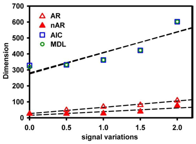
Estimated signal dimensions for simulated group datasets are plotted as a function of intragroup signal variations, which are characterized by the strength of the random fluctuations added into the 16 independent signal sources across all subgroup datasets in the simulation. A positive linear dependence between the estimated dimensions and the signal variations is shown. Traditional prenoise methods like AIC and MDL generally report much higher dimensions than the known individual signal dimension of 16. The proposed postnoise AR(1) fitting method (nAR) demonstrates the least dependence on the increasing signal variations among the subgroup datasets.

4. Discussion

We have presented an improved technique for estimating the signal dimensions of multilevel group fMRI data sets. As we have demonstrated, the proposed method can be used for single-level and multilevel data reductions, which would be important for large-scale group analysis. Another application is specifying the appropriate number of signal components in data-driven analyses such as ICA algorithm [2], providing an essential basis for group-level ICA. We have employed the proposed method in several internal projects using ICA to explore the functional networks in the human brain (see Chen et al. [23] for example).

Our analysis has shown that substantial overestimation of signal dimensions occurs for group fMRI data with traditional methods and that this problem is primarily caused by spectral changes in the group data compared to the original subgroup data sets. In our opinion, these spectral alterations can be introduced by either intragroup signal variations or the data reduction process in producing the group data. Therefore, we propose a noise-blurring approach to overcome this problem by adding artificially generated autoregressive noise to the group data to ensure that the postnoise group data have a spectral structure similar to those of the original prereduction data sets, and then the postnoise group data can be subjected to regular dimension methods that are assumed to be valid for the individual fMRI data sets. Our results indicated that the greatest protection against dimension overestimation is obtained with the AR(1) fitting technique [15], while the proposed approach actually can help any dimension estimation technique. We would like to note that the autoregressive structure and the strength of the added blurring noise can be uniquely determined with respect to the average spectrum of original subgroup data sets. It is also empirically suggested that this blurring noise is unlikely to cause an overcorrection to the dimension overestimation under the conditions described.

The dimension overestimation for group fMRI data is usually demonstrated by a significant linear dependence of the estimated signal dimensions on varying group sizes. In practice, this linear dependence may lead to a gigantic group data volume that cannot be handled in an ordinary computer system and/or the difficulty of comparing data-driven analysis results from groups with different sizes. Our data have shown that, compared with other methods, the proposed postnoise AR(1) fitting method (nAR) provides the dimension estimation with the least dependence on group sizes. Nevertheless, we acknowledge that there could be alternative strategies to eliminating the dependence of dimension estimations on group sizes. For example, rather than applying the dimension methods to the group data, we may simply use the average of estimated individual dimensions as a representative of the group. In our opinion, however, this method may not be ideal for group data dimension estimation because information on intragroup signal variations is totally lost. Moreover, this averaging strategy does not deal with the spectral alterations caused by data reduction; thus, it is difficult to employ for multilevel group data sets.

Other approaches to mitigating the problem of signal variations are also possible. For example, intensive spatial smoothing applied to group data is an alternative strategy to blur intragroup variations [8]. However, we believe that the proposed method is superior in the following aspects. (1) The noise-blurring technique can suppress intragroup variation in both spatial and temporal domains simultaneously, whereas the spatial smoothing technique generally works in the spatial domain only, or, if both are applied, it would be difficult to determine an appropriate smoothing ratio between the two domains. (2) The parameters of blurring noise can be uniquely determined in a process to compensate for the spectral alterations of the group data with respect to the original subgroup data sets. In contrast, spatial smoothing lacks such an objective criterion for determining the smoothing parameters. (3) The proposed noise-blurring technique can work at all levels of group data, whereas there is no evidence on the spatial smoothing technique’s effectiveness in multilevel group data.

As there have been extensive studies on the mathematical basis of the classic dimension estimation theory (for a review, see Friston et al. [24] and Worsley and Friston [25]), we chose to present our method primarily in the framework of the AR(1) fitting technique, that is, using the divergent point between the fitted noise PCA spectrum and the actual data PCA spectrum to indicate the signal dimension of the data. This is not only because AR(1) fitting provides an intuitive explanation to the dimension estimation problem but also because the proposed noise-blurring technique displays the best performance when combined with AR(1) fitting. The postnoise MDL method, for example, can provide dimension estimations smaller than the total number of data points in the group. However, compared to the AR(1) fitting method, the postnoise MDL method shows greater sensitivity to group size and reports higher dimensionality estimations for the second and third levels. More importantly, the superior performance of the proposed postnoise AR(1) fitting technique is also justified by the greater constancy at the third level between the two different grouping orders, where, presumably, information content should be identical. However, for both prenoise and postnoise AR(1) fitting techniques, the dimension results at the second level are larger and less variable in the “scan–subject–session” order. This is because each intersubject group comprises N=14 individual data sets, whereas the intersession group comprises only M=5 elements. Interestingly, the regular AR(1) fitting method gives a second-level dimension estimation that is slightly larger than that of the third level in the “scan–subject–session” order. This unreasonable result may reflect the unsuitability of the regular AR(1) fitting method for dealing with multilevel group fMRI data. Unlike the regular method, the estimated dimension from the proposed post-noise AR(1) fitting technique is consistently larger at the third level than at the second level.

For future work, we would like to explore the neurophysiological basis of the dimension measurements of the fMRI data. Under the premise that the brain connectivity networks derived from spontaneous fluctuations in resting-state fMRI signals have been reported to follow specific brain circuits, including sensorimotor, visual, auditory and language processing networks [3,26–31], we speculate that the signal dimension of fMRI data acquired from the brain may represent the total “volume” or “complexity” of the functional networks in the resting brain, as revealed by previous multivariate data-driven studies using ICA and PCA methods. Thus, it would be interesting to further investigate if the signal dimension of fMRI data would be associated with the status of brain activities.

5. Conclusion

Traditional dimension methods substantially overestimate the signal dimension of group fMRI data. The proposed postnoise AR(1) fitting technique addressed this problem by using an autoregressive noise-blurring technique to suppress the intragroup signal variations and data-reduction-induced spectral alterations that contribute to the dimension overestimation. Our data indicated that the proposed method significantly reduced the dimension overestimation for group fMRI data at multiple data reduction levels and exhibited good consistency between the different grouping orders.

Appendix A. Supplementary data

Supplementary data associated with this article can be found, in the online version, at doi:10.1016/j.mri.2010.04.002.

References

- 1.Hansen LK, Larsen J, Nielsen FA, Strother SC, Rostru E, Savoy R, et al. Generalizable patterns in neuroimaging: how many principal components? NeuroImage. 1999;9:534–44. doi: 10.1006/nimg.1998.0425. [DOI] [PubMed] [Google Scholar]
- 2.Calhoun VD, Adali T, Pearlson GD, Pekar JJ. A method for making group inferences from functional MRI data using independent component analysis. Hum Brain Mapp. 2001;14:140–51. doi: 10.1002/hbm.1048. [DOI] [PMC free article] [PubMed] [Google Scholar]
- 3.Beckmann CF, DeLuca M, Devlin JT, Smith SM. Investigations into resting-state connectivity using independent component analysis. Philos Trans R Soc Lond B Biol Sci. 2005;360:1001–13. doi: 10.1098/rstb.2005.1634. [DOI] [PMC free article] [PubMed] [Google Scholar]
- 4.Damoiseaux JS, Rombouts SA, Barkhof F, Scheltens P, Stam CJ, Smith SM, et al. Consistent resting-state networks across healthy subjects. Proc Natl Acad Sci U S A. 2006;103:13848–53. doi: 10.1073/pnas.0601417103. [DOI] [PMC free article] [PubMed] [Google Scholar]
- 5.Calhoun VD, Kiehl KA, Pearlson GD. Modulation of temporally coherent brain networks estimated using ICA at rest and during cognitive tasks. Hum Brain Mapp. 2008;29(7):828–38. doi: 10.1002/hbm.20581. [DOI] [PMC free article] [PubMed] [Google Scholar]
- 6.Esposito F, Aragri A, Pesaresi I, Cirillo S, Tedeschi G, Marciano E, et al. Independent component model of the default-mode brain function: combining individual-level and population-level analyses in resting-state fMRI. Magn Reson Imaging. 2008;26(7):905–13. doi: 10.1016/j.mri.2008.01.045. [DOI] [PubMed] [Google Scholar]
- 7.Beckmann CF, Smith SM. Probabilistic independent component analysis for functional magnetic resonance imaging. IEEE Trans Med Imaging. 2004;23:137–52. doi: 10.1109/TMI.2003.822821. [DOI] [PubMed] [Google Scholar]
- 8.Li Y, Calhoun VD. Sample dependence correction for order selection in fMRI analysis. IEEE International Symposium on Biomedical Imaging: Nano to Macro; 2006. pp. 1072–5. [Google Scholar]
- 9.Minka TP. MIT media laboratory perceptual computing section technical report no. 514. Cambridge, MA: MIT Media Laboratory Perceptual Computing Section Technical Report; 2000. Automatic choice of dimensionality for PCA. [Google Scholar]
- 10.Meindl T, Teipel S, Elmouden R, Mueller S, Koch W, Dietrich O, et al. Test-retest reproducibility of the default-mode network in healthy individuals. Hum Brain Mapp. 2010;31(2):237–46. doi: 10.1002/hbm.20860. [DOI] [PMC free article] [PubMed] [Google Scholar]
- 11.Akaike H. A new look at statistical model identification. IEEE Trans Automat Contr AC. 1974;19:716–23. [Google Scholar]
- 12.Weakliem DL. A critique of the Bayesian information criterion for model selection. Sociol Methods Res. 1999;27(3):359–97. [Google Scholar]
- 13.Rissanen J. A universal prior for integers and estimation by minimum description length. Ann Stat. 1983;11:416–31. [Google Scholar]
- 14.Maxim V, Sendur L, Fadili J, Suckling J, Gould R, Howard R, et al. Fractional Gaussian noise, functional MRI and Alzheimer’s disease. NeuroImage. 2005;25(1):141–58. doi: 10.1016/j.neuroimage.2004.10.044. [DOI] [PubMed] [Google Scholar]
- 15.Cordes D, Nandy RR. Estimation of the intrinsic dimensionality of fMRI data. NeuroImage. 2006;29:145–54. doi: 10.1016/j.neuroimage.2005.07.054. [DOI] [PubMed] [Google Scholar]
- 16.Beckmann CF, Noble J, Smith S. Investigating the intrinsic dimensionality of fMRI data for ICA. 7th International Conference on Functional Mapping of the Human Brain; Brighton, UK. 2001. [Google Scholar]
- 17.Thirion B, Pinel P, Meriaux S, Roche A, Dehaene S, Poline J. Analysis of a large fMRI cohort: statistical and methodological issues for group analyses. NeuroImage. 2007;35:105–20. doi: 10.1016/j.neuroimage.2006.11.054. [DOI] [PubMed] [Google Scholar]
- 18.Wax M, Kailath T. Detection of signals by information theoretic criteria. IEEE Trans Acoust Speech Signal Process. 1985;33(2):387–92. [Google Scholar]
- 19.Talairach J, Tournoux P. Co-planar stereotaxic atlas of the human brain. New York: Thieme; 1988. [Google Scholar]
- 20.Cox RW. AFNI: software for analysis and visualization of functional magnetic resonance neuroimages. Comput Biomed Res. 1996;29:162–73. doi: 10.1006/cbmr.1996.0014. [DOI] [PubMed] [Google Scholar]
- 21.Svensen M, Kruggel F, Benali H. ICA of fMRI group study data. NeuroImage. 2002;16:551–63. doi: 10.1006/nimg.2002.1122. [DOI] [PubMed] [Google Scholar]
- 22.Van de Ven VG, Formisano E, Prvulovic D, Roeder CH, Linden DEJ. Functional connectivity as revealed by spatial independent component analysis of fMRI measurements during rest. Hum Brain Mapp. 2004;22:165–78. doi: 10.1002/hbm.20022. [DOI] [PMC free article] [PubMed] [Google Scholar]
- 23.Chen S, Ross T, Zhan W, Myers C, Chuang KS, Heishman S, et al. Group independent component analysis reveals consistent resting-state networks across multiple sessions. Brain Res. 2008;1239:141–51. doi: 10.1016/j.brainres.2008.08.028. [DOI] [PMC free article] [PubMed] [Google Scholar]
- 24.Friston KJ, Holmes A, Poline J, Grasby P, Williams S, Frackowiak R, et al. Analysis of fMRI time series revisited. NeuroImage. 1995;2:45–53. doi: 10.1006/nimg.1995.1007. [DOI] [PubMed] [Google Scholar]
- 25.Worsley K, Friston K. Analysis of fMRI time series revisited — again. NeuroImage. 1995;2:173–81. doi: 10.1006/nimg.1995.1023. [DOI] [PubMed] [Google Scholar]
- 26.Biswal B, Yetkin FZ, Haughton VM, Hyde JS. Functional connectivity in the motor cortex of resting human brain using echo-planar MRI. Magn Reson Med. 1995;34:537–41. doi: 10.1002/mrm.1910340409. [DOI] [PubMed] [Google Scholar]
- 27.Lowe MJ, Mock BJ, Sorenson JA. Functional connectivity in single and multislice echoplanar imaging using resting-state fluctuations. NeuroImage. 1998;7:119–32. doi: 10.1006/nimg.1997.0315. [DOI] [PubMed] [Google Scholar]
- 28.Xiong J, Parsons LM, Gao JH, Fox PT. Interregional connectivity to primary motor cortex revealed using MRI resting state images. Hum Brain Mapp. 1999;8:151–6. doi: 10.1002/(SICI)1097-0193(1999)8:2/3<151::AID-HBM13>3.0.CO;2-5. [DOI] [PMC free article] [PubMed] [Google Scholar]
- 29.Cordes D, Haughton VM, Arfanakis K, Wendt GJ, Turski PA, Moritz CH, et al. Mapping functionally related regions of brain with functional connectivity MR imaging. AJNR Am J Neuroradiol. 2000;2:1636–44. [PMC free article] [PubMed] [Google Scholar]
- 30.Greicius MD, Krasnow B, Reiss AL, Menon V. Functional connectivity in the resting brain: a network analysis of the default mode hypothesis. Proc Natl Acad Sci U S A. 2003;100:253–8. doi: 10.1073/pnas.0135058100. [DOI] [PMC free article] [PubMed] [Google Scholar]
- 31.Fox MD, Snyder AZ, Vincent JL, Corbetta M, Van Essen DC, Raichle ME. The human brain is intrinsically organized into dynamic, anticorrelated functional networks. Proc Natl Acad Sci U S A. 2005;102:9673–8. doi: 10.1073/pnas.0504136102. [DOI] [PMC free article] [PubMed] [Google Scholar]
Associated Data
This section collects any data citations, data availability statements, or supplementary materials included in this article.