

Abstract
As high-throughput biochemical screens are both expensive and labor intensive, researchers in academia and industry are turning increasingly to virtual-screening methodologies. Virtual screening relies on scoring functions to quickly assess ligand potency. Although useful for in silico ligand identification, these scoring functions generally give many false positives and negatives; indeed, a properly trained human being can often assess ligand potency by visual inspection with greater accuracy. Given the success of the human mind at protein−ligand complex characterization, we present here a scoring function based on a neural network, a computational model that attempts to simulate, albeit inadequately, the microscopic organization of the brain. Computer-aided drug design depends on fast and accurate scoring functions to aid in the identification of small-molecule ligands. The scoring function presented here, used either on its own or in conjunction with other more traditional functions, could prove useful in future drug-discovery efforts.
Introduction
High-throughput biochemical screens, used to identify pharmacologically active small-molecule compounds, are a staple of modern drug discovery. In these screens, hundreds of thousands to even millions of compounds are tested in highly automated assays. Although robotics and miniaturization have led to increased efficiency, traditional high-throughput screens are nevertheless expensive and labor intensive. With a few notable exceptions, the financial and labor requirements of such screens place them beyond the reach of most academic institutions.
Consequently, academic researchers, as well as some in industry, are increasingly turning to virtual screens. Virtual screens rely on computer docking programs to position models of potential ligands within target active sites and predict the binding affinity. Precise physics-based computational techniques for binding-energy prediction, such as thermodynamic integration,1,2 single-step perturbation,(3) and free energy perturbation,(4) are too time- and calculation-intensive for use in virtual screens. Instead, researchers have developed simpler scoring functions that sacrifice some accuracy in favor of greater speed.5−7 Because of these accepted inaccuracies, scoring functions are unable to explicitly identify ligands in silico; rather, they serve only to enrich the pool of candidate ligands with potential hits. The compounds with the best predicted binding energies are subsequently tested in experimental assays to verify activity.
Current scoring functions fall into three general classes.(8) The first class, based on molecular force fields, predicts binding energy by estimating electrostatic and van der Waals forces explicitly. Docking programs using force-field-based scoring functions include AutoDock,(1) Dock,(9) Glide,10,11 ICM,(12) and Gold (GoldScore).(13) A second class of “empirical” scoring functions include those used by Glide10,11 and eHits (SFe empirical scoring function),14,15 as well as the ChemScore(16) and Piecewise Linear Potential (PLP)(17) functions. These functions estimate binding energy by calculating the weighted sum of all hydrogen-bond and hydrophobic contacts. A third class of scoring function, called “knowledge based,” relies on statistical analyses of crystal-structure databases. Pairs of atom types that are frequently found in close proximity are judged to be energetically favorable. Examples include the Astex Statistical Potential (ASP)(18) and the SFs statistical scoring function used by eHits.14,15
These approaches to binding-affinity prediction have proven very useful; virtual-screening efforts routinely identify predicted ligands that are subsequently validated experimentally (see, for example, refs (19) and (20)). However, modern scoring functions produce many false-positive and false-negative results. Surprisingly, a human being with the proper training can often analyze a docked structure visually and correctly assess inhibition with greater accuracy.(8) Remarkably, the human mind can characterize ligand binding without employing physical or chemical equations and without requiring the explicit calculation of affinity constants. Although any computational model pales in comparison to the complexity of the brain, the mind’s ability to categorize protein−ligand complexes nevertheless suggests that a neural network, a computer model designed to mimic the microscopic organization of the brain, might be at least as suited to the prediction of protein−ligand binding affinities as equation- and statistics-based scoring functions.
Herein, we describe a fast and accurate neural-network-based scoring function that can be used to rescore the docked poses of candidate ligands. The function is in some ways knowledge based, as it draws upon protein-structure databases to “learn” what structural characteristics favorably affect binding. However, the use of neural networks in this context is largely unprecedented.(21) Although useful in its own right, the neural-network approach to affinity prediction is also orthogonal to existing physics-based and statistics-based scoring functions and, so, might prove useful in consensus-scoring projects as well.
Results and Discussion
Neural networks are computer models designed to mimic, albeit inadequately, the microscopic architecture and organization of the brain. In brief, various “neurodes,” analogous to biological neurons, are joined by “connections,” analogous to neuronal synapses. The behavior of the network is determined not only by the organization and number of the neurodes, but also by the weights (i.e., strengths) of the connections.
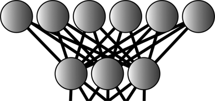
All neural networks have at least two layers. The first, called the input layer, receives information about the system the network is to analyze. The second, called the output layer, encodes the results of that analysis. Additionally, optional hidden layers receive input from the input layer and transmit it to the output layer, allowing for even more complex behavior (Figure 1).
Figure 1.

Schematic of a simple neural network. All neural networks have an input layer, through which information about the system to be analyzed is passed, and an output layer, which encodes the results of the analysis. Optional hidden layers receive input from the input layer and transmit it to the output layer, allowing for even more complex behavior.
In designing a neural network to analyze a complex data set, the specific formulas that describe the relationships between data-set characteristics need not be explicitly delineated; rather, the designer need only provide the network with an adequate description of the system so that the network can infer those relationships on its own. In the current context, creating neural networks to characterize the binding affinity of protein−ligand complexes does not require that we implement or even understand the specific formulaic relationships that describe van der Waals, electrostatic, and hydrogen-bond interactions, though the energies calculated by these formulas can in theory be included in the network input.(21) Rather, we must determine what characteristics of a protein−ligand complex the network needs to “see” in order to correctly analyze and characterize the complex on its own.
What Properties of a Protein−Ligand Complex Determine Binding Affinity?
Ligand binding affinity is determined by both enthalpic and entropic factors. Specific atom−atom interactions, including electrostatic, hydrogen-bond, van der Waals, π−π, and π−cation interactions, contribute to the enthalpic component of the binding energy. In contrast, the entropic contribution is determined in part by the number of ligand rotatable bonds and the challenges of disordering and rearranging the ordered hydration shells surrounding the unbound ligand and the apo active site. The entropic penalty related to hydration is difficult to calculate explicitly and is likely a function of many factors, including the hydrophobicity and volume of the ligand, the number of buried but unsatisfied hydrogen-bond donors and acceptors upon binding, and the protein−ligand contact surface area. In the current work, we therefore sought to identify the characteristics of protein−ligand complexes that might affect these enthalpic and entropic factors.
First, the proximity of ligand and protein atoms likely contributes to the binding affinity by affecting enthalpic factors (i.e., electrostatic, van der Waals, hydrogen-bond, π−π, and π−cation interactions), as well as entropic factors (i.e., buried but unsatisfied hydrogen bonds and the size of the protein−ligand contact area). In the current context, this proximity information is stored in a proximity list. The distances between the atoms of the ligand and the protein are considered; atoms that are close to each other are subsequently grouped by their corresponding AutoDock atom types, and the number of each atom-type pair is tallied.
Second, electrostatic interactions contribute to the enthalpic component of the binding energy through salt bridges and hydrogen bonds. The electrostatic energy is certainly dependent on proximity, but it is also dependent on partial atomic charges. Consequently, for each of the atom-type pairs in the proximity list described above, a summed electrostatic energy is also calculated from the assigned Gasteiger charges.
Third, certain ligand characteristics related to the quantity and identity of ligand atom types, such as ligand hydrophobicity and volume, could affect the entropy of binding as well. Consequently, all of the atoms of the ligand are categorized by their corresponding atom types. Finally, the number of rotatable bonds in the ligand is explicitly counted, as ligand flexibility can also have an important impact on entropy.
Developing Neural Networks to Analyze These Properties of Protein−Ligand Complexes
When all of these atom-type pairs, ligand atom types, and other metrics are considered separately, a given protein−ligand complex can be characterized across 194 dimensions; thus, we created neural networks with input layers containing 194 neurodes. As output, only two neurodes are needed to distinguish between good and poor binders: (1, 0) indicates that a given protein−ligand complex has a dissociation constant Kd < 25 μM, and (0, 1) indicates that a given complex has Kd > 25 μM. Although somewhat arbitrary, our experience with virtual screening has led us to believe that 25 μM is a reasonable cutoff for distinguishing between inhibitors that warrant further study and optimization and poor inhibitors that are best not pursued further.
To train candidate neural networks, 4141 protein−ligand complexes were downloaded from the Protein Data Bank(22) and characterized across the 194 dimensions described above. These 4141 complexes included 2695 unique, diverse protein structures mapping to over 600 UniProt primary accession numbers. Of these 4141 complexes, 2710 had Kd values that had been experimentally measured; 2022 of these were good binders (Kd < 25 μM), and 688 were poor binders (Kd ≥ 25 μM). Recognizing that the poor binders were underrepresented, additional complexes of poorly binding ligands were obtained by docking compounds of the NCI Diversity Set II into the same protein receptors as used previously. One thousand four hundred thirty-one of these dockings into 571 unique PDB structures had highest-ranked ligand poses with predicted binding energies between 0 and −4 kcal/mol. These were also included in the database of protein−ligand complexes as examples of weak binders.
Preliminary Studies to Validate the Model
Multiple neural networks were trained to study the influence of network architecture and training-set size on accuracy and to judge the robustness of the network output. Ultimately, a network architecture consisting of a single hidden layer of five neurodes was selected. Training sets of 1, 10, 25, 50, 100, 250, 500, 1000, 2000, 3000, and 4000 protein−ligand complexes were generated by randomly selecting complexes from among the 4141 complexes previously characterized. Random training sets were generated for each network to ensure that network accuracy was independent of the complexes chosen for inclusion. In all cases, the remaining complexes were used as a validation set to verify that the networks had not been overtrained and to judge training effectiveness.
Each individual network has its own unique strengths and weaknesses; to obtain consistent results across multiple protein−ligand complexes, it is better to take the average prediction of multiple networks rather than to trust the prediction of any single network. For each training-set size described above, we therefore trained 10 independent neural networks and averaged the corresponding outputs (Figure 2).
Figure 2.
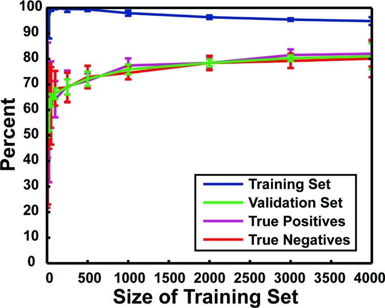
Accuracy of protein−ligand complex characterization. The x axis shows the size of the training set, and the y axis shows the percent accuracy. Each data point represents the average accuracy of 10 independent neural networks with one hidden layer of five neurodes. Error bars represent standard deviations. In blue are shown the accuracies with which the various networks were able to characterize the binding constants of the protein−ligand complexes in their respective training sets. In green are shown the accuracies with which the various networks were able to characterize the binding constants of the complexes in their respective validation sets. In purple is shown the likelihood that a given protein−ligand complex has a Kd value less than 25 μM given that the network predicts high-affinity binding (i.e., the true-positive rate when the respective validation sets were analyzed). In red is shown the likelihood that a given protein−ligand complex has a binding affinity greater than 25 μM given that the network predicts poor binding (i.e., the true-negative rate when the respective validation sets were analyzed).
Figure 2 depicts the accuracy of these neural networks, that is, the frequency with which they accurately characterized the protein−ligand complexes of their respective training and validation sets as either having high affinity (Kd < 25 μM) or low affinity (Kd > 25 μM). Although trained to give a binary response [(1, 0) for strong binding, (0, 1) for weak binding], network output was in fact continuous [(a, b), where a + b = 1.0 because network outputs were normalized]. To evaluate each protein−ligand complex, a score (n = a − b) was calculated. If n > 0, the network output was interpreted to predict Kd < 25 μM; otherwise, it predicted Kd > 25 μM.
The accuracy with which the networks were able to characterize the binding constants of the protein−ligand complexes in their respective training sets (i.e., those complexes to which the network had already been “exposed”) is shown in Figure 2, in blue. Interestingly, training-set accuracy was good regardless of training-set size.
The networks’ ability to correctly characterize the protein−ligand complexes of their respective validation sets, sets comprising complexes that had never been seen before, was far more indicative of true predictive ability. The accuracies of these predictions (Figure 2, in green) clearly demonstrate that overtraining had not occurred, as accuracy consistently improved with exposure to larger training sets. After having been exposed to only 1000 examples, the networks were already quite good at characterizing protein−ligand complexes; however, additional examples did result in moderate improvements in accuracy. We note also that, for training-set sizes greater than 1000, the standard deviation of the outputs of the 10 networks associated with each training-set size was relatively small, suggesting that network output was largely independent of the training set selected. The single best network of all those tested correctly characterized the protein−ligand complexes of its training and validation sets with 94.8% and 87.9% accuracy, respectively.
Accuracy can be divided into two parts. The true-positive rate (Figure 2, in purple) indicates the likelihood that a given protein−ligand complex has a Kd value less than 25 μM given that the network predicts high-affinity binding. The true-negative rate (Figure 2, in red) indicates the likelihood that a given protein−ligand complex has a binding affinity greater than 25 μM given that the network predicts poor binding. The true-positive and true-negative rates of these networks are roughly equal regardless of training-set size; these networks are just as good at identifying true inhibitors as they are at identifying poor ones.
Training Additional Networks to Improve Accuracy
Having confirmed that the networks were not overtrained and that network output was robust regardless of the composition of the training sets, we next sought to train additional networks to determine whether accuracy could be improved. Ten networks with training sets of 4000 randomly selected complexes were generated in the preliminary studies described above. To determine whether even more accurate networks could be trained, we generated an additional 1000 independent neural networks with similar training sets of 4000 randomly selected protein−ligand complexes. In each case, the remaining 141 complexes were again used as a validation set. Three of these 1000 networks emerged as the most accurate (89.4% accuracy on the validation set); 24 had validation-set accuracies greater than 87.5%.
Recalling that each network is unique and that consistent results are best obtained when the average prediction of multiple networks is considered, we defined a single score, called an NNScore (N), obtained by averaging the outputs of these 24 networks.
Can N Be Used as a Scoring Function?
To assess how the NNScore (N) varied according to the experimentally measured Kd values, we considered the scores of the 2710 characterized protein−ligand complexes with known Kd values described above. To facilitate visualization, the data were ordered by the log10(Kd) value. Moving averages of both the log10(Kd) values and the associated N values were calculated over 100 points and are plotted in Figure 3. Unaveraged data points are shown as gray circles. It is interesting to note that the data-averaged function crosses the x axis at roughly 25 μM [log10(25 × 10−6) = −4.60], as expected. So remarkable is this result that one again wonders whether the networks were overtrained; however, as Figure 2 demonstrates, these networks were consistently able to predict the binding of ligands to which they had never been exposed, suggesting the development of a genuine inductive bias.
Figure 3.

Average score (N) over 24 networks as a function of the experimentally measured Kd value. To facilitate visualization, the data were ordered by log10(Kd) value. Moving averages of both the log10(Kd) values and the associated N values were calculated over 100 points. This data-averaged function (shown in black) crosses the x axis at 25 μM [log10(25 × 10−6) = −4.60, shown as a dotted line]. Individual, unaveraged data points are shown in gray.
Despite the fact that the networks were trained to answer what is essentially a yes-or-no question, Figure 3 demonstrates that they can nevertheless perceive certain “shades of gray”, that is, they can distinguish not only between good and poor binders, but, to a certain extent, even between good and better binders. Given that N decreases somewhat monotonically as log10(Kd) increases, it might therefore be possible to use N as a scoring function.
Can N Distinguish between Well- and Poorly Docked Ligands?
A good scoring function should be able to distinguish between ligands that are well docked and ligands that are poorly docked. To determine whether or not the NNScore could make this distinction, we generated a database of poorly docked ligands separate from the training/testing database described above. Selected ligands from the 4141 previously characterized protein−ligand complexes were redocked back into their corresponding receptors using AutoDock Vina.(23) In 287 cases, the predicted binding energy of the worst-docked pose was greater than −4 kcal/mol. These 287 worst-docked poses, together with their associated protein receptors, were included in the poorly docked database.
The top three neural networks of the 1000 generated were each used to characterize these 287 poorly docked binding poses. These three networks correctly identified the ligands as poor binders 94.1%, 88.9%, and 95.5% of the time. Thus, despite the fact that these three networks characterized the protein−ligand complexes of their respective validation sets with the same accuracy, they were somewhat less consistent when presented with new data. Under most circumstances, it is not possible to know a priori which network is best suited for a given database of protein−ligand complexes; a more consistent result can be obtained by considering the average score over multiple networks (N). Indeed, when the average score over the top 24 networks was used to characterize these protein−ligand complexes, an accuracy of 94.1% was achieved.
Can N Distinguish between True and False Binders When Both Are Well Docked?
Although the networks were successful at identifying poorly docked ligands, the ability to distinguish between true high-affinity binders and poor binders when both are well docked is far more challenging. To test the networks’ abilities, we docked 103 small-molecule compounds into the active site of influenza N1 neuraminidase (N1, PDB ID: 3B7E)(24) using AutoDock Vina.(23) Three of these compounds were known neuraminidase inhibitors: oseltamivir, peramivir, and zanamivir. The remaining 100 ligands were decoys selected at random from the NCI Diversity Set II. We note that, of the 4141 protein−ligand complexes used in the training and validation sets, one consisted of zanamivir bound to N1, and two consisted of oseltamivir bound to N1. However, no examples of peramivir bound to N1 were present in the Protein Data Bank;(22) the networks had never been exposed to this protein−ligand complex.
The results of this small virtual screen are shown in Table 1. When the AutoDock Vina scoring function(23) was used to rank the compounds, the known inhibitors ranked 5th, 10th, and 55th. When the docked poses were rescored using each of the top three individual neural networks, the known inhibitors fared substantially better, with the predicted poorest binder ranking 24th, 31st, and 9th, respectively. One of the individual neural networks performed particularly well, ranking the known inhibitors second, eighth, and ninth. However, this network could not have been identified a priori. When the compounds were ranked by the average score over the top 24 networks (N), the known inhibitors performed equally well. Had the top 10 compounds from this virtual screen been subsequently tested experimentally, only the network-based scoring functions would have permitted the identification of all three inhibitors. The enrichment factor of such a virtual screen would have been 10.3.
Table 1. Results of a Small Virtual Screen against Influenza N1 Neuraminidase Used to Test the Novel Neural-Network Scoring Functiona.
| top 10b | EFc | rankZMRd | rankOMRe | rankPMRf | |
|---|---|---|---|---|---|
| Vina | 2/3 | 6.9 | 10 | 55 | 5 |
| NN1 | 2/3 | 6.9 | 24 | 4 | 1 |
| NN2 | 1/3 | 3.4 | 16 | 31 | 1 |
| NN3 | 3/3 | 10.3 | 8 | 9 | 2 |
| N (average24) | 3/3 | 10.3 | 7 | 10 | 2 |
Five scoring functions compared: AutoDock Vina score, predictions of the top three individual neural networks (NN1, NN2, and NN3, respectively), and average prediction of the top 24 networks (N).
Number of known inhibitors that ranked in the top ten for each scoring function.
Enrichment factor when the top 10 ligands were considered.
Rank of the known inhibitor zanamivir.
Rank of the known inhibitor oseltamivir.
Rank of the known inhibitor peramivir.
To further validate the predictive potential of these neural networks, we repeated the above virtual-screening protocol using a crystal structure of T. brucei RNA editing ligase 1 (TbREL1), a protein that was not included in the 4141 protein−ligand complexes used in the training and validation sets. As three positive controls (i.e., known inhibitors), we chose ATP, the natural substrate, and compounds V1 and S5, TbREL1 inhibitors recently identified by Amaro et al.(19) When the compounds were ranked by the average NNScore score over the top 24 networks (N), two of the three known inhibitors ranked in the top ten, giving an enrichment factor of 6.87. This enrichment was equal to that obtained when the compounds were ranked by the Vina scoring function (Table 2).
Table 2. Results of a Small Virtual Screen against Tb REL1 Used to Test the Novel Neural-Network Scoring Functiona.
| top 10b | EFc | rankATPd | rankV1e | rankS5f | |
|---|---|---|---|---|---|
| Vina | 2/3 | 6.9 | 8 | 18 | 9 |
| NN1 | 1/3 | 3.4 | 99 | 2 | 25 |
| NN2 | 1/3 | 3.4 | 2 | 16 | 24 |
| NN3 | 2/3 | 6.9 | 7 | 1 | 69 |
| N (average24) | 2/3 | 6.9 | 8 | 5 | 27 |
Five scoring functions compared: AutoDock Vina score, predictions of the top three individual neural networks (NN1, NN2, and NN3, respectively), and average prediction of the top 24 networks (N).
Number of known inhibitors that ranked in the top 10 for each scoring function.
Enrichment factor when the top 10 ligands were considered.
Rank of the known inhibitor ATP.
Rank of the known inhibitor V1.
Rank of the known inhibitor S5.
This second screen illustrates several important points. First, as mentioned above, each of the individual networks has its own unique strengths and weaknesses. For example, the network labeled NN1 was far better at identifying compound V1 than was Vina, NN2 was better at identifying ATP, and NN3 was better at identifying both ATP and V1 (Table 2). As we could not have known a priori which network is best suited for this system, it is wise not to trust the results of any single network. When the compounds were ranked by the average output of the top 24 networks, ATP and V1 still ranked in the top 10 compounds, but the result was not dependent on a single network output.
A second point of interest illustrated by this screen is that, for at least some systems, the networks’ unique approach to binding-affinity prediction might be orthogonal to more traditional approaches. For example, in this second screen, Vina identified S5 as a true binder, but the networks did not; in contrast, the networks tended to be better at identifying V1 and, with the notable exception of NN1, ATP. By using the networks in conjunction with Vina, perhaps a useful consensus score could be developed.
To test this hypothesis, a consensus score for each compound was calculated by averaging the ranks obtained when the Vina score and the NNScore score were used. When the compounds were reranked by this consensus score, ATP, V1, and S5 ranked first, second, and eighth, respectively. Assuming that the top 10 predicted inhibitors were subsequently tested experimentally, ranking by this consensus score would yield an enrichment factor of 10.3, superior to the enrichment obtained when the compounds were ranked by the Vina scoring function or the network outputs alone. We recommend using positive controls (i.e., known inhibitors) to determine whether a single scoring function or a consensus score is best suited to a given virtual-screening project.
Conclusions
The research presented here demonstrates that neural networks can be used to successfully characterize the binding affinities of protein−ligand complexes. Not only were these networks able to distinguish between well-docked and poorly docked ligands, they were also able to distinguish between true ligands and decoy compounds when both were well docked. A user-friendly scoring function based on these networks has been implemented in Python and can be downloaded from http://www.nbcr.net/software/nnscore.
Although the networks’ success with the neuraminidase and TbREL1 systems was promising, predictive accuracy might be system dependent. Regardless, one strength of the neural-network scoring function is that it is largely orthogonal to other kinds of functions based on force fields, linear regression, and statistical analyses. Thus, in many cases, it could be useful to rank by consensus scores that combine neural-network scoring functions with other more traditional functions.
Experimental Section
Training/Testing Database Preparation
To build a database of protein−ligand complexes of known binding affinity, we identified X-ray crystal and NMR structures from the Protein Data Bank (PDB)(22) that had Kd values listed in the MOAD(25) and PDBbind-CN26,27 databases. Where multiple similar Kd values were present in these databases, Kd values were averaged to give one value per protein−ligand complex. Where multiple differing Kd values were present, the corresponding complex was discarded. Additionally, complexes with peptide or DNA ligands, ligands with rare atom types (e.g., gold, copper, iron, zinc), receptors with rare ligand-binding atom types (e.g., copper, nickel, cobalt), and complexes with Kd values greater than 0.5 M were likewise discarded. Ultimately, 2710 complexes remained.
Hydrogen atoms were added to the ligands of these complexes using Schrödinger Maestro (Schrödinger). All protonation states were verified by visual inspection. For those complexes with ligand-binding metal cations, the partial charge of each metal atom was assigned to be the formal charge. The geometries of the hydrogen bonds between the ligand and the receptor were optimized using an in-house script. AutoDockTools 1.5.1(28) was used to add hydrogen atoms to the receptors, to merge nonpolar hydrogen atoms with their parent atoms, and to assign atom types and Gasteiger charges. The ligand was likewise processed with AutoDockTools.
Most of the protein−ligand interactions listed in the MOAD and PDBbind-CN databases were high-affinity; of those used in the current study, for example, only about 25% had Kd values greater than 25 μM. To include adequate examples of weak-binding ligands, 20 randomly selected ligands from the NCI Diversity Set II, a set of freely available, diverse compounds provided by the Developmental Therapeutics Program (NCI/NIH), were docked into each of the receptors described above using AutoDock Vina.(23) In all, 1431 ligands with best predicted binding energies between 0 and −4 kcal/mol were identified and included in the database as examples of weak-binding ligands.
Poorly Docked Database Preparation
In addition to the database of crystallographic and well-docked poses described above, we also generated a separate database of poorly docked protein−ligand complexes. Some of the ligands of the training/testing database described above were docked back into their corresponding receptors using AutoDock Vina.(23) Rather than identifying the ligand pose with the best predicted binding energy, the pose with the worst predicted binding energy was considered. In 287 cases, this worst predicted binding energy was greater than −4 kcal/mol; these 287 protein−ligand complexes were included in the poorly docked database.
Influenza Neuraminidase Database Preparation
To create a database of compounds docked into influenza neuraminidase, three known neuraminidase inhibitors (oseltamivir, peramivir, and zanamivir) were docked into a neuraminidase crystal structure obtained from the PDB (PDB ID: 3B7E).(24) Additionally, 100 compounds were randomly selected from the NCI Diversity Set II to serve as decoys. All 103 compounds were docked into the neuraminidase active site using AutoDock Vina.(23)
TbREL1 Database Preparation
A database of compounds docked into TbREL1 was similarly generated. Three known ligands (ATP, V1, and S5(19)) were docked into a TbREL1 crystal structure (PDB ID: 1XDN).(29) As before, 100 compounds were randomly selected from the NCI Diversity Set II to serve as decoys.
Characterization of Protein−Ligand Complexes
All protein−ligand complexes were characterized in four ways. First, close protein−ligand contacts were considered. Pairs of ligand and protein atoms within 2 Å of each other were first identified. These protein−ligand atom pairs were then characterized according to the AutoDock atom types of their two constituents, and the number of each of these close-contact atom-type pairs was tallied in a list. Fourteen protein−ligand atom-type pairs were permitted: (A, HD), (C, HD), (C, OA), (C, SA), (FE, HD), (HD, HD), (HD, MG), (HD, N), (HD, NA), (HD, OA), (HD, ZN), (MG, OA), (NA, ZN), and (OA, ZN).
A similar list of close-contact atom-type pairs was tallied for all protein−ligand atom pairs within 4 Å of each other. Eighty-three atom-type pairs were permitted: (A, A), (A, BR), (A, C), (A, CL), (A, F), (A, FE), (A, HD), (A, I), (A, N), (A, NA), (A, OA), (A, P), (A, S), (A, SA), (A, ZN), (BR, C), (BR, HD), (BR, N), (BR, OA), (C, C), (C, CL), (C, F), (C, FE), (C, HD), (C, I), (CL, HD), (CL, N), (CL, OA), (CL, SA), (C, MG), (C, MN), (C, N), (C, NA), (C, OA), (C, P), (C, S), (C, SA), (C, ZN), (FE, HD), (FE, N), (FE, OA), (F, HD), (F, N), (F, OA), (F, SA), (HD, HD), (HD, I), (HD, MG), (HD, MN), (HD, N), (HD, NA), (HD, OA), (HD, P), (HD, S), (HD, SA), (HD, ZN), (I, N), (I, OA), (MG, NA), (MG, OA), (MG, P), (MN, N), (MN, OA), (MN, P), (NA, OA), (NA, SA), (NA, ZN), (N, N), (N, NA), (N, OA), (N, P), (N, S), (N, SA), (N, ZN), (OA, OA), (OA, P), (OA, S), (OA, SA), (OA, ZN), (P, ZN), (SA, SA), (SA, ZN), and (S, ZN).
Second, the electrostatic-interaction energy between protein and ligand atoms within 4 Å of each other was calculated and summed for each of the atom-type pairs described above:
where qr is the partial charge of receptor atom r, ql is the partial charge of ligand atom l, and d is the distance between the two. The same atom-type pairs permitted for close-contact protein−ligand atoms within 4 Å of each other were again used.
Third, a list of ligand atom types was likewise tallied, and the number of atoms of each type was counted. Thirteen ligand atom types were permitted: A, BR, C, CL, F, HD, I, N, NA, OA, P, S, and SA. Finally, the number of ligand rotatable bonds was likewise counted. In all, each protein−ligand complex was thus characterized across 194 (14 + 83 + 83 + 13 + 1) dimensions.
Neural-Network Setup
All neural networks were feed-forward networks created using FFNET(30) with 194 inputs and 2 outputs. All nodes in the hidden and output layers had log-sigmoid activation functions of the form
where t is the input sum of the respective node. Network inputs and outputs were normalized with a linear mapping to the range (0.15, 0.85) so that each variable was given equal initial importance independent of its scale. There were no direct connections between the input and output layers; all nodes of the hidden layer were connected to all nodes of the input layer, and all nodes of the output layer were connected to all nodes of the hidden layer.
The networks were trained to return (1, 0) for protein−ligand complexes with experimentally measured Kd values less than 25 μM, and (0, 1) for complexes with Kd values greater than 25 μM. To train each network, the weights of the connections between neurodes were first randomly assigned; these weights were subsequently optimized by applying 10000 steps of a constrained truncated Newton algorithm(31) as implemented in SciPy.(32)
Training sets of varying sizes were employed. In all cases, training sets consisted of protein−ligand complexes picked at random from the 4141 complexes of the training/testing database described above. The remaining complexes constituted the validation set, used to judge the network’s predictive accuracy.
Abbreviations: EF, enrichment factor; NCI, National Cancer Institute; NIH, National Institutes of Health; PDB, Protein Data Bank.
Acknowledgments
J.D.D. was funded by a Pharmacology Training Grant through the UCSD School of Medicine. This work was also carried out with funding from Grants NIH GM31749, NSF MCB-0506593, and MCA93S013 to J.A.M. Additional support from the Howard Hughes Medical Institute, the National Center for Supercomputing Applications, the San Diego Supercomputer Center, the W. M. Keck Foundation, the National Biomedical Computational Resource, and the Center for Theoretical Biological Physics is gratefully acknowledged.
Funding Statement
National Institutes of Health, United States
References
- Morris G. M.; Goodsell D. S.; Halliday R. S.; Huey R.; Hart W. E.; Belew R. K.; Olson A. J. Automated docking using a Lamarckian genetic algorithm and an empirical binding free energy function. J. Comput. Chem. 1998, 19, 1639–1662. [Google Scholar]
- Oostenbrink B. C.; Pitera J. W.; van Lipzig M. M.; Meerman J. H.; van Gunsteren W. F. Simulations of the estrogen receptor ligand-binding domain: Affinity of natural ligands and xenoestrogens. J. Med. Chem. 2000, 43, 4594–605. [DOI] [PubMed] [Google Scholar]
- Oostenbrink C.; van Gunsteren W. F. Free energies of binding of polychlorinated biphenyls to the estrogen receptor from a single simulation. Proteins 2004, 54, 237–246. [DOI] [PubMed] [Google Scholar]
- Kim J. T.; Hamilton A. D.; Bailey C. M.; Domaoal R. A.; Wang L.; Anderson K. S.; Jorgensen W. L. FEP-guided selection of bicyclic heterocycles in lead optimization for non-nucleoside inhibitors of HIV-1 reverse transcriptase. J. Am. Chem. Soc. 2006, 128, 15372–15373. [DOI] [PubMed] [Google Scholar]
- Marrone T. J.; Briggs J. M.; McCammon J. A. Structure-based drug design: Computational advances. Annu. Rev. Pharmacol. Toxicol. 1997, 37, 71–90. [DOI] [PubMed] [Google Scholar]
- Wong C. F.; McCammon J. A. Protein flexibility and computer-aided drug design. Annu. Rev. Pharmacol. Toxicol. 2003, 43, 31–45. [DOI] [PubMed] [Google Scholar]
- McCammon J. A.Computer-Aided Drug Discovery: Physics-based Simulations from the Molecular to the Cellular Level. In Physical Biology: From Atoms to Medicine; Zewail A. H., Ed.; World Scientific Publishing: Singapore, 2008; pp 401−410. [Google Scholar]
- Schulz-Gasch T.; Stahl M. Scoring functions for protein−ligand interactions: A critical perspective. Drug Discov. Today: Technol. 2004, 1, 231–239. [DOI] [PubMed] [Google Scholar]
- Ewing T. J.; Makino S.; Skillman A. G.; Kuntz I. D. DOCK 4.0: Search strategies for automated molecular docking of flexible molecule databases. J. Comput.-Aided Mol. Des. 2001, 15, 411–428. [DOI] [PubMed] [Google Scholar]
- Friesner R. A.; Banks J. L.; Murphy R. B.; Halgren T. A.; Klicic J. J.; Mainz D. T.; Repasky M. P.; Knoll E. H.; Shelley M.; Perry J. K.; Shaw D. E.; Francis P.; Shenkin P. S. Glide: A new approach for rapid, accurate docking and scoring. 1. Method and assessment of docking accuracy. J. Med. Chem. 2004, 47, 1739–1749. [DOI] [PubMed] [Google Scholar]
- Halgren T. A.; Murphy R. B.; Friesner R. A.; Beard H. S.; Frye L. L.; Pollard W. T.; Banks J. L. Glide: A new approach for rapid, accurate docking and scoring. 2. Enrichment factors in database screening. J. Med. Chem. 2004, 47, 1750–1759. [DOI] [PubMed] [Google Scholar]
- Totrov M.; Abagyan R. Flexible protein−ligand docking by global energy optimization in internal coordinates. Proteins 1997, 215–220Suppl 1. [DOI] [PubMed] [Google Scholar]
- Jones G.; Willett P.; Glen R. C.; Leach A. R.; Taylor R. Development and validation of a genetic algorithm for flexible docking. J. Mol. Biol. 1997, 267, 727–748. [DOI] [PubMed] [Google Scholar]
- Zsoldos Z.; Reid D.; Simon A.; Sadjad B. S.; Johnson A. P. eHiTS: An innovative approach to the docking and scoring function problems. Curr. Protein Pept. Sci. 2006, 7, 421–435. [DOI] [PubMed] [Google Scholar]
- Zsoldos Z.; Reid D.; Simon A.; Sadjad S. B.; Johnson A. P. eHiTS: A new fast, exhaustive flexible ligand docking system. J. Mol. Graphics Modell. 2007, 26, 198–212. [DOI] [PubMed] [Google Scholar]
- Eldridge M. D.; Murray C. W.; Auton T. R.; Paolini G. V.; Mee R. P. Empirical scoring functions: I. The development of a fast empirical scoring function to estimate the binding affinity of ligands in receptor complexes. J. Comput.-Aided Mol. Des. 1997, 11, 425–445. [DOI] [PubMed] [Google Scholar]
- Gehlhaar D. K.; Verkhivker G. M.; Rejto P. A.; Sherman C. J.; Fogel D. B.; Fogel L. J.; Freer S. T. Molecular recognition of the inhibitor AG-1343 by HIV-1 protease: Conformationally flexible docking by evolutionary programming. Chem. Biol. 1995, 2, 317–324. [DOI] [PubMed] [Google Scholar]
- Mooij W. T.; Verdonk M. L. General and targeted statistical potentials for protein−ligand interactions. Proteins 2005, 61, 272–287. [DOI] [PubMed] [Google Scholar]
- Amaro R. E.; Schnaufer A.; Interthal H.; Hol W.; Stuart K. D.; McCammon J. A. Discovery of drug-like inhibitors of an essential RNA-editing ligase in Trypanosoma brucei. Proc. Natl. Acad. Sci. U.S.A. 2008, 105, 17278–17283. [DOI] [PMC free article] [PubMed] [Google Scholar]
- Durrant J. D.; Urbaniak M. D.; Ferguson M. A.; McCammon J. A. Computer-Aided Identification of Trypanosoma brucei Uridine Diphosphate Galactose 4′-Epimerase Inhibitors: Toward the Development of Novel Therapies for African Sleeping Sickness. J. Med. Chem. 2010, 53, 5025–5032. [DOI] [PMC free article] [PubMed] [Google Scholar]
- Artemenko N. Distance dependent scoring function for describing protein−ligand intermolecular interactions. J. Chem. Inf. Model. 2008, 48, 569–574. [DOI] [PubMed] [Google Scholar]
- Berman H. M.; Westbrook J.; Feng Z.; Gilliland G.; Bhat T. N.; Weissig H.; Shindyalov I. N.; Bourne P. E. The Protein Data Bank. Nucleic Acids Res. 2000, 28, 235–242. [DOI] [PMC free article] [PubMed] [Google Scholar]
- Trott O.; Olson A. J. AutoDock Vina: Improving the speed and accuracy of docking with a new scoring function, efficient optimization, and multithreading. J. Comput. Chem. 2009, 31, 455–461. [DOI] [PMC free article] [PubMed] [Google Scholar]
- Xu X.; Zhu X.; Dwek R. A.; Stevens J.; Wilson I. A. Structural characterization of the 1918 influenza virus H1N1 neuraminidase. J. Virol. 2008, 82, 10493–10501. [DOI] [PMC free article] [PubMed] [Google Scholar]
- Hu L.; Benson M. L.; Smith R. D.; Lerner M. G.; Carlson H. A. Binding MOAD (Mother of All Databases). Proteins 2005, 60, 333–340. [DOI] [PubMed] [Google Scholar]
- Wang R.; Fang X.; Lu Y.; Wang S. The PDBbind database: Collection of binding affinities for protein−ligand complexes with known three-dimensional structures. J. Med. Chem. 2004, 47, 2977–2980. [DOI] [PubMed] [Google Scholar]
- Wang R.; Fang X.; Lu Y.; Yang C. Y.; Wang S. The PDBbind database: Methodologies and updates. J. Med. Chem. 2005, 48, 4111–4119. [DOI] [PubMed] [Google Scholar]
- Sanner M. F. Python: A programming language for software integration and development. J. Mol. Graphics Modell. 1999, 17, 57–61. [PubMed] [Google Scholar]
- Deng J.; Schnaufer A.; Salavati R.; Stuart K. D.; Hol W. G. High resolution crystal structure of a key editosome enzyme from Trypanosoma brucei: RNA editing ligase 1. J. Mol. Biol. 2004, 343, 601–613. [DOI] [PubMed] [Google Scholar]
- Wojciechowski M.FFNET: Feed-Forward Neural Network for Python, 0.6; Technical University of Łódź: Łódź, Poland, 2007. [Google Scholar]
- Nash S. G. Newton-like minimization via the Lanczos method. SIAM J. Numer. Anal. 1984, 21, 770–788. [Google Scholar]
- Peterson P. F2PY: A tool for connecting Fortran and Python programs. Int. J. Comput. Sci. Eng. 2009, 4, 296–305. [Google Scholar]