Hierarchical Auditory Processing Directed Rostrally along the Monkey's Supratemporal Plane

Abstract

Connectional anatomical evidence suggests that the auditory core, containing the tonotopic areas A1, R, and RT, constitutes the first stage of auditory cortical processing, with feedforward projections from core outward, first to the surrounding auditory belt and then to the parabelt. Connectional evidence also raises the possibility that the core itself is serially organized, with feedforward projections from A1 to R and with additional projections, although of unknown feed direction, from R to RT. We hypothesized that area RT together with more rostral parts of the supratemporal plane (rSTP) form the anterior extension of a rostrally directed stimulus quality processing stream originating in the auditory core area A1. Here, we analyzed auditory responses of single neurons in three different sectors distributed caudorostrally along the supratemporal plane (STP): sector I, mainly area A1; sector II, mainly area RT; and sector III, principally RTp (the rostrotemporal polar area), including cortex located 3 mm from the temporal tip. Mean onset latency of excitation responses and stimulus selectivity to monkey calls and other sounds, both simple and complex, increased progressively from sector I to III. Also, whereas cells in sector I responded with significantly higher firing rates to the “other” sounds than to monkey calls, those in sectors II and III responded at the same rate to both stimulus types. The pattern of results supports the proposal that the STP contains a rostrally directed, hierarchically organized auditory processing stream, with gradually increasing stimulus selectivity, and that this stream extends from the primary auditory area to the temporal pole.

Introduction

Neuroimaging studies in monkeys (Poremba and Mishkin, 2007; Petkov et al., 2008) raise the possibility that, like occipitotemporal visual areas, superior temporal auditory areas send highly processed stimulus quality information to downstream targets via a multisynaptic corticocortical pathway that proceeds stepwise in a caudorostral direction. Yet most of the evidence that has been gathered regarding serial auditory processing points to information flow orthogonal to the caudorostral axis.

In monkeys, the medial geniculate nucleus sends projections to the auditory core areas (A1, R, and RT) on the supratemporal plane (STP), which then project to their laterally and medially adjacent neighbors in the auditory belt, and these, in turn, project laterally to the auditory parabelt (Galaburda and Pandya, 1983; Kaas and Hackett, 2000). The evidence thus suggests that the core constitutes the first stage of cortical processing, with a serial progression from core outward, first to the belt and then to the parabelt. This schema is supported by electrophysiological findings. Rauschecker and colleagues (Rauschecker et al., 1995; Rauschecker and Tian, 2000, 2004; Tian et al., 2001; Tian and Rauschecker, 2004) showed that neurons in the anterolateral belt area (AL) are much more responsive to such sounds as bandpassed noise, frequency-modulated (FM) sweeps, and monkey calls than they are to pure tones, suggesting that area AL is at a higher level of processing than medially adjacent core area R. Moreover, area AL is a source of direct projections to the ventrolateral prefrontal cortex (Petrides and Pandya, 1988; Hackett et al., 1999; Romanski et al., 1999a,b), where neurons also respond to complex sounds, including monkey vocalizations (Romanski and Goldman-Rakic, 2002; Cohen et al., 2004; Gifford et al., 2005; Romanski et al., 2005; Russ et al., 2008), suggesting that area AL is a late modality-specific cortical station for processing stimulus quality.

However, with the exception of recent findings in marmosets (Bendor and Wang, 2008), little is known regarding the neuronal properties of the rostral superior temporal region, including the rostral part of the supratemporal plane (rSTP), raising the question of what contribution, if any, this region makes to the processing of complex sounds. Yet this rostral region (1) receives inputs from more caudal superior temporal areas (Hackett et al., 1998; de la Mothe et al., 2006), and, in the case of rSTP, receives caudal inputs from serially organized core areas A1 and R (Fitzpatrick and Imig, 1980; Galaburda and Pandya, 1983), (2) serves auditory discrimination and auditory short-term memory functions (Strominger et al., 1980; Fritz et al., 2005), and (3) appears to play a special role in processing conspecific calls (Poremba et al., 2004; Petkov et al., 2008). To explore the possibility that the rostral region, and the rSTP in particular, contains the anterior extension of a rostrally directed auditory pathway, we compared the responses of rSTP and A1 neurons to a wide variety of sounds. Our aim was to determine whether rSTP neurons have properties expected of cells in a higher auditory area, such as longer latencies, more complex receptive fields, and more selective tuning than do neurons in A1.

Materials and Methods

Subjects.

Two adult male rhesus monkeys (Macaca mulatta) weighing 6–8.5 kg were used. All procedures and animal care were conducted in accordance with the Institute of Laboratory Animal Resources Guide for the Care and Use of Laboratory Animals, and all experimental procedures were approved by the National Institute of Mental Health Animal Care and Use Committee. The monkeys received audiological screening (monkey A while awake, and B while in a sedated condition), which included both DPOAE (distortion product otoacoustic emission) to assess cochlear function and tympanometry to evaluate middle ear function. The hearing ability of both monkeys was assessed as normal.

Behavioral task and acoustic stimuli.

Behavioral testing and recording sessions were conducted in a double-walled acoustic chamber (Industrial Acoustic Company) installed with foam isolation (AAP3; Acoustical Solutions). The animal sat in a monkey chair with its head fixed, facing a free-field speaker (JBL) (see below) located ∼60 cm directly in front of it in a darkened room. The animal was trained to perform an auditory discrimination task, mainly to ensure that it attended to the sounds during the recording sessions. A single positive stimulus (S+), consisting of a 300 ms burst of white noise, was pseudorandomly interspersed among 40 other sounds, all of which were negative (S−). To respond correctly, the monkey thus had to attend to at least the onset or a segment of each sound. The animal initiated a trial by holding a lever for 500 ms, triggering the presentation of one of the 41 stimuli. Lever release within a 500 ms response window after offset of the S+ led to a water reward (∼0.2 ml) followed by a 500 ms intertrial interval (ITI). Lever release to any of the 40 S− sounds prolonged the 500 ms ITI by 1 s. The 500 ms lever hold period that triggered the next stimulus began only when the intertrial interval ended.

The 40 S− stimuli, the spectrograms of which are illustrated in Figure 1, where they are described in detail, consisted of 20 rhesus monkey calls (MCs) and 20 other auditory (OA) stimuli. The 20 MC stimuli included different versions of barks, screams, coos, grunts, and warbles. The 20 OA stimuli consisted of environmental sounds, nonprimate vocalizations, and synthesized stimuli, including complex frequency-amplitude-modulated sounds, FM sweeps, and pure tones. The mean duration of the S− stimuli was 0.48 s (range, 0.17–1.48 s). The amplitude of the S+ stimulus was 67 dB sound pressure level (SPL) after RMS normalization, and that of the S− stimuli ranged from 60 to 73 dB SPL (“A”-frequency and fast-time weighted, measured with a Bruel & Kjaer integrating sound level meter, model 2237, and a 1.27 cm type 4137 prepolarized free-field condenser microphone mounted on a tripod at the location of the animal's ear). The stimulus waveforms were attenuated (PA4; Tucker-Davis Technologies), amplified (STA-130; Realistic), and played through the loudspeaker (N24AW; JBL). The speaker had a flat (±3 dB) frequency response from 75 Hz to 20 kHz.

Figure 1.

The single S+ stimulus (not illustrated) was a 300 ms white noise. The 40 S− stimuli (illustrated here) consisted of 20 rhesus MCs (top panel, sounds 1–20) and 20 OA stimuli (bottom panel, sounds 21–40). Some of the MC stimuli were recorded on Cayo Santiago, Puerto Rico (provided courtesy of M. D. Hauser, Harvard University, Cambridge, MA), and the others, in the Laboratory of Neuropsychology, National Institute of Mental Health (Poremba et al., 2004); these 20 calls consisted of the following: shrill bark (1; numerals in parentheses refer to sound number), bark (2, 4, 6, 7, 12), pulse scream (5), scream (11, 16, 19), scream plus coo (20), coo (8, 14, 15), coo combination (18), grunt (3, 9), grunt plus coo (10), and gurney warble (13, 17). The OA stimuli consisted of the following: four environmental sounds (21–24) (e.g., slamming of a cage door); five nonprimate vocalizations (25–29) (e.g., human, dog, crow; Nature 99 Sound Effects, SFX); and 11 synthesized sounds, each 300 ms long. These 11 synthesized sounds included the following: two complex, frequency-and-amplitude-modulated sounds (30–31); six FM sweeps (32–37), two ascending from 1 to 5 and 1 to 10 kHz, two descending from 5 to 1 and 10 to 1 kHz, and two both ascending and descending from 1 to 5 and 5 to 1 kHz, and from 1 to 10 and 10 to 1 kHz, interspersed with a steady-state portion for 100 ms; and three pure tones (38–40), 1, 5, and 10 kHz. For the different sound categories, the mean durations (and ranges) were as follows: monkey calls, 0.48 s (0.17–1.00 s); environmental sounds, 1.03 s (0.61–1.48 s); nonprimate vocalizations, 0.35 s (0.27–0.57 s); and synthesized sounds, 0.31 s (0.26–0.42 s), with a mean duration for all S− sounds of 0.48 s. All spectrograms were displayed with linear frequency on the vertical axis and time on the horizontal axis. A sound envelope with a 5 ms rise/fall linear function was applied to all the sounds.

Within each 200 trial block of the discrimination task, all 40 S− sounds were presented four times each for a total of 160 trials, interspersed pseudorandomly with 40 S+ sounds presented on average once every five trials. In recording from each site, an attempt was made to present the 200 trial block five times in succession, in a different random order each time. Since, normally, one trial took an average of 2.5 s (range, 1.2–3.5 s), a 1000 trial session at a given site lasted ∼40 min. The animals performed the auditory discrimination task at 95% accuracy (80.7% correct responses for the 20% S+ trials, and 98.6% correct for the 80% S− trials). Most (18.3%) of the errors were failures to release the lever to the S+ stimulus, and these occurred mainly in the latter part of a recording session, reflecting satiation and/or fatigue rather than discrimination difficulty. The other types of error were either premature responses to the S+ sound [lever release before sound offset (1.0%)] or lever release to an S− sound (1.4%). Analyses of neuronal activity presented below are based on recordings taken from correct trials only.

Animal preparation and electrophysiological recording.

To stabilize the animal's performance, training on the auditory discrimination task was continued for ∼8 months, after which the animal was anesthetized and a head post and recording chamber were attached under aseptic conditions to the dorsal surface of the skull. The chamber (65° angle; Crist Instruments) was positioned stereotaxically over the left hemisphere with guidance from a magnetic resonance imaging (MRI) scan (1.5 tesla MRI scanner; 1 mm³ voxel size; GE). We implanted chambers over the rostral part of the left temporal lobe in both monkeys and a chamber over the caudal part of the left temporal lobe in monkey A after the rostral chamber was removed. On confirmation with MRI that the chamber was positioned correctly, a skull disc within the chamber was removed under aseptic conditions to allow the later insertion of microelectrodes through a stainless-steel guide tube (23 gauge; FHC).

Before each recording session, a reference point above the STP was calculated, based on the MRI images and the coordinates mapped onto the chamber; then the guide tube holding four tungsten microelectrodes (9–12 MΩ at 1 kHz; shank diameter, 100 μm; Epoxylite insulation, ∼50 μm thick; FHC) was lowered to this reference point by use of a remote-controlled, four-channel, microstep hydraulic multidrive system (MCU-4; FHC). The four electrodes were in a 2 × 2 arrangement and spaced 190 μm apart horizontally. Each electrode was then independently advanced, and the depth where the first robust spontaneous activity was observed was set as the reference point for that electrode. Different recording sites within each electrode track were separated vertically by at least 200 μm, to ensure that the recordings were from different cells.

The electrode signals were amplified and filtered between 100 and 8000 Hz by a preamplifier system (PBX2/16sp; Plexon) to remove local field potentials. Action potentials were monitored visually on an oscilloscope (Hameg; HM407-2) and audibly from the speaker outside the sound chamber. Action potentials were sorted by the spike sorting software (Offline Sorter; Plexon). PC1 and PC2 were calculated by principal component analysis to distinguish different spike shapes from different cells, and the Valley Seeking algorithm was used in two-dimensional feature space for cluster cutting. When more than one cluster was found, the degree of separation of the clusters was tested by multivariate ANOVA at p < 0.01, and if it met the criterion, the cluster was designated as single-unit activity. Trains with interspike intervals less than the refractory period (1 ms) were also removed. Since recording at each site usually required ∼40 min, the recording sometimes became unstable because of electrode drift. Such unstable spike trains appeared as a discontinuous cluster in time and were excluded from analysis. If the spike sorting did not yield clear clustering above the criterion, the activity was categorized as multiunit activity. For data analysis in the present study, we grouped the single-unit and multiunit activity together. Signals indicating the timing of auditory stimulus, behavioral response, and reward events were sent through CORTEX (CIO-DAS1602/12; CIO-DIO24; ComputerBoards) to a multichannel acquisition processor system (MAP; Plexon), and integrated with the spike data at a sampling rate of 40 kHz. The acquired spike-timing and event-timing data were exported to Matlab (The MathWorks) for additional analysis.

Data analysis.

The spike trains of each neuron were convolved with a Gaussian kernel (σ = 10) to construct peristimulus time histograms (PSTHs), which were then normalized to the average variability (SD) of the spontaneous firing rate for 500 ms before stimulus onset across the prestimulus periods of all the trials for all 40 S− sounds. Stimulus-evoked activity that was 2.8 SD or more above this baseline activity (p = 0.005) for 10 consecutive 1 ms bins was designated an excitation response, whereas a significant decrease of mean firing rate below baseline activity across ∼20 trials (p < 0.01 by the Wilcoxon signed rank test) was designated a suppression response. We defined a neuron as “auditory responsive” if at least one of the stimuli elicited an excitation or a suppression response that met the above criteria.

For each auditory neuron that showed an excitation response to at least one sound, we calculated the total number of effective sounds (Nef) (i.e., the number of sounds that met the excitation criterion). Similarly, for each neuron that produced a suppression response to at least one sound, we calculated a Nef for suppression.

We also calculated for each neuron the onset and minimum latencies of each excitation response, as well as the latency to the peak response of the neuron. Onset latency was defined as the time from sound onset to the first millisecond bin that rose 2 SD above baseline for 10 consecutive 1 ms bins, provided this occurred within 165 ms, the duration of our shortest S− stimulus (sound 1, a monkey vocalization). This restriction on the duration of the temporal window in the calculation of onset latency helped reduce such contaminants as sound-offset responses to short-duration sounds and phasic responses locked to certain acoustic features appearing in the middle of complex sounds. Minimum latency was defined as the shortest onset latency elicited by any of the S− stimuli to which the neuron responded. We performed a separate minimum-latency calculation for neurons that showed a significant response to at least one of three pure tones (sounds 38–40), and in this case we did not apply the time window restriction to detect the onset latency as all the sounds shared the same envelope shapes and sound duration (300 ms). Peak latency was defined as the time at which excitation in the spike density function reached its maximum (a latency used only to calculate peak response firing rates, as described below).

Finally, we calculated for each neuron both the mean and peak response magnitudes for each excitation response. Mean response magnitude was defined as the mean firing rate for the full duration of the sound. Peak magnitude was defined as the average firing rate for 25 ms on either side of the peak latency and, separately, for 50 ms on either side of the peak latency (i.e., response windows of 50 and 100 ms, respectively). Both response magnitudes were defined as firing rates above the baseline activity of the neuron.

Results

Division of neurons by sector

We recorded from a total of 571 neurons in the two monkeys. All the cells were located in the left STP (including the inferior bank of the circular sulcus) between 3 and 22 mm from the temporal pole and 19–26 mm lateral to the midline (Fig. 2). Since our aim was to compare the acoustic properties of neurons distributed along the caudorostral dimension of the supratemporal plane, we divided the recordings into three caudorostrally distributed sectors, approximately equal to each other in caudorostral extent and neuronal number.

Figure 2.

Location of recording sites on the STP. A, Standard lateral view of left hemisphere depicting anterior–posterior (AP) extent of the three sectors (I, II, and III marked in red, green, and blue, respectively). Numerals above bars indicate distance in millimeters anterior to AP0 measured along the stereotaxic horizontal plane. B, The location of the three sectors depicted on the left STP of monkey A, color-coded as in A. Note that the vertical plane 3 mm posterior to the temporal pole corresponds to the vertical plane 25 mm anterior to AP0. Cir, Circular sulcus. C, Top panels, Sites of auditory cells represented by yellow dots on the coronal MR images at the indicated AP levels, shown for each of the two monkeys separately. Bottom panels, The full coronal MR images (A–C) correspond to the partial coronal images with the same labels in the top panels.

As indicated in the figure, sector I neurons (190 of 571; 33%) were located in an area 6–10 mm rostral to the interaural plane or AP0; sector II neurons (182 of 571; 32%), in an area 17–20 mm rostral to AP0; and sector III neurons (199 of 571; 35%), in an area 21–25 mm rostral to AP0. Based on a comparison between these AP levels on the MRI scans and cytoarchitectonic maps of the supratemporal plane, we estimate that sector I neurons were located primarily within the caudal-to-middle portion of the primary auditory core area, A1, although the most caudolateral recording sites could have encroached on the lateral belt; sector II, mainly within the anterior portions of auditory core area RT (Saleem and Logothetis, 2007) [or in the region of TS2 in the terminology of Galaburda and Pandya (1983)]; and sector III, primarily within area RTp (Saleem and Logothetis, 2007) [or in the region of TS1 in the terminology of Galaburda and Pandya (1983)].

Of the 571 STP neurons, 396 (69%) responded significantly above or below baseline firing rates (see Materials and Methods, Data analysis) to at least one of the 41 sounds (1 S+ and 40 S− sounds) (Fig. 1). Among these 396 neurons, 34 neurons responded to the S+ sound only (sector I, 8 neurons; sector II, 9 neurons; sector III, 17 neurons). Because the S+ was associated with nonacoustic factors [expectation of reward as well as preparation for manual and oromotor responses (i.e., lever release and drinking)], we excluded these 34 neurons from additional analysis, focusing on the 362 neurons that responded to at least one of the 40 S− sounds. These 362 neurons were distributed among the three sectors as follows: sector I, 143 (40%); sector II, 134 (37%); sector III, 85 (23%). Approximately one-half of these were single units, and the other one-half, multiunits (see Materials and Methods, Animal preparation and electrophysiological recording). Finally, within each sector, the proportions of recorded neurons that were responsive to one or more of our auditory stimuli were as follows: sector I, 75% (143 of 190); sector II, 74% (134 of 182); and sector III, 43% (85 of 199).

Sample neuron from each sector

Before presenting the statistical analyses comparing the acoustic properties of the neuronal populations in the three different sectors, we describe the stimulus-evoked responses of a sample neuron from each sector (Fig. 3) to illustrate how the acoustic properties were measured.

Figure 3.

Responses of three illustrative neurons in columns A–C, one neuron from each of the three sectors. Average poststimulus time histograms (PSTHs) aligned to sound onset (vertical red line). Sound spectrogram is displayed on top of the panel aligned to sound onset and offset. The left y-axis is in spikes/second and the right y-axis indicates SD units above or below baseline activity (defined in text). Response of cell in A to sound 16 (scream) and sound 40 (10 kHz tone); response of cell in B to sound 17 (warble) and sound 31 (complex stimulus); and response of cell in C to sound 11 (scream) and sound 18 (coo). D, Normalized peak (black bar) and mean (white bar) firing rate to each of the 40 S− sounds for the cell in A; E, same for the cell in B; and F, same for the cell in C. The y-axes in D–F show the normalized firing rate above baseline activity. The asterisk indicates significant excitation response. MC (1–20), Monkey calls; OA (21–40), other auditory stimuli; Nef, number of effective sounds (defined in text). G, Location of cells in A–C. Cir, Circular sulcus.

The sample neuron in sector I, located in area A1 ∼20 mm from the temporal pole (Fig. 3G), exhibited significant excitation responses to 32 of the 40 stimuli (19 monkey vocalizations and 13 other auditory stimuli) (Fig. 3D); the responses to two of these are illustrated in Figure 3A. The onset latency of this neuron was 27 ms to the scream (top panel, sound 16) and 22 ms to the 10 kHz pure tone (bottom panel, sound 40), to which it showed its highest mean firing rate (Fig. 3D) (mean, 39.8 and 43.3 spikes/s for sounds 16 and 40, respectively; baseline, 13.1 spikes/s). Additional examination of the firing characteristics of this neuron indicated that its responses to monkey calls, such as the warble, as well as to other complex sounds were likely driven by sound frequencies that, like the 10 kHz tone, had sufficient power at, or close to, its preferred frequency (supplemental Fig. 1, available at www.jneurosci.org as supplemental material).

In comparison, neurons in sectors II and III tended to be more selective to the sounds, sometimes responding to monkey calls preferentially (Fig. 3B,E) or, even more selectively, to a single monkey call (Fig. 3C,F). Thus, the sample sector II neuron, located 9 mm from the temporal pole in the region of RT, showed significant excitation responses to seven monkey vocalizations and to four other auditory stimuli (Fig. 3E). As illustrated in Figure 3B, its responses to the warble (sound 17, its best stimulus, with mean and peak firing rates of 6.7 and 16.6 spikes/s, respectively; baseline, 2.7 spikes/s) had an onset latency of 203 ms, reliably longer than the 37 ms onset latency of the sector 1 sample neuron to the same sound (supplemental Fig. 1, available at www.jneurosci.org as supplemental material). The responses of this neuron to a subset of the monkey calls might have been driven not by a preferred single frequency (indeed, it responded to none of the single tones or sweeps we used) (supplemental Fig. 2, available at www.jneurosci.org as supplemental material). The apparent preference of the unit for stimuli with complex features, a set shared in part by many of the monkey calls (Fig. 4A), resulted in significantly higher mean and peak firing rates for all 20 MC stimuli than those for all 20 OA stimuli (Fig. 4B) (MC vs OA, mean rate, 3.3 ± 1.4 vs 2.3 ± 1.4 spikes/s; p < 0.02; peak rate, 9.1 ± 3.5 vs 6.2 ± 2.6 spikes/s; p < 0.01; Wilcoxon's signed rank test). A similar pattern of responses from another sector II neuron is illustrated in supplemental Figure 3 (available at www.jneurosci.org as supplemental material).

Figure 4.

Response profile of the sector II neuron illustrated in Figure 3. A, Bars indicate the peak response magnitudes of this cell (defined in text) evoked by each of the 40 S− sounds, arranged in rank order. Of the 10 stimuli that evoked the highest peak firing rates, 9 were monkey calls; the response of this cell to its best stimulus (sound 17, warble) is illustrated in Figure 3B. B, Curves show the average PSTH of this cell to the 7 effective MC stimuli, the 4 effective OA stimuli, and the 29 ineffective stimuli, as shown in Figure 3E.

In the case of the illustrated sector III neuron (Fig. 3C,F), which was located 6 mm from the temporal pole in the region of RTp (Fig. 3G), the scream (sound 11) was the only monkey call that elicited an excitation response, and one that was very delayed (onset and peak latencies, 194 and 213 ms, respectively). Although the second highest response of this neuron to an S− stimulus did not reach the response criterion, note that this sound was also a monkey vocalization (coo, sound 18) (Fig. 3C, bottom panel).

Population comparison of neuronal response properties across the three sectors

Response type

Neurons were first classified on the basis of whether they were excited or suppressed by the sounds (response type). Of the 362 auditory responsive neurons, 170 (47%) showed excitation only, firing significantly above baseline to all the sounds to which they were responsive; 103 (28%) showed suppression only, firing significantly below baseline to all the sounds to which they were responsive; and 89 (25%) were of the mixed-response type, firing significantly above baseline to one or more of the sounds and significantly below baseline to one or more of the other sounds.

As illustrated in Figure 5, both excitation-only and mixed responses fell progressively across the three sectors, with sector I having the largest percentage of these two response types and sector III, the smallest. Conversely, suppression-only responses rose progressively across the sectors, with sector I having the smallest percentage of this response type, and sector III, the largest. Using χ² tests, we compared these widely differing proportions of each response type with the predicted proportion of each (based on the overall percentages listed above), and for each response type we found significant differences among the three sectors (excitation only, χ² = 11.28; mixed, χ² = 12.55; suppression only, χ² = 54.92; all values of p < 0.01) (for examples of suppression responses, see supplemental Fig. 4, available at www.jneurosci.org as supplemental material).

Figure 5.

Proportion of auditory neurons within each sector classified by response type. Excitation only, Each neuron in this category had firing rates significantly above baseline to all the sounds to which it was responsive. Suppression only, Each neuron in this category had firing rates significantly below baseline to all the sounds to which it was responsive. Mixed, Each neuron in this category showed excitation to one or more stimuli and suppression to one or more others. χ² tests indicated that the proportions of each response type within a sector differed significantly across the sectors (see text) (Table 1).

Stimulus selectivity

We next compared stimulus selectivity across the three sectors by calculating for each neuron the number of S− sounds that elicited a significant excitation response (Nef) (Table 1; supplemental Fig. 5, available at www.jneurosci.org as supplemental material). Figure 6A shows the Nef for excitation responses plotted on the grids of the three sectors. This mean Nef decreased progressively as the recording sites moved rostrally: sector I, 6.23 ± 0.64 (mean ± SEM), N = 128; sector II, 5.44 ± 0.58, N = 100; and sector III, 1.84 ± 0.27, N = 31. A two-way repeated-measures ANOVA showed a main effect of recording site (F_(2,256) = 6.21; p < 0.01) but not of stimulus category or of the interaction between these two factors. Post hoc paired comparisons revealed a significantly lower Nef in sector III than in each of the other sectors (Tukey's honestly significant difference test, values of p < 0.001). As shown in Figure 6C, similar results were obtained when Nef was calculated separately for the two stimulus categories, monkey calls and other auditory stimuli (MC, p < 0.02; OA, p < 0.01). Within the MC category, the stimulus selectivity of sector III neurons was especially high, 45% (14 of 31 activated cells) having responded significantly to but a single monkey call, compared with 17% (17 of 100) in sector II, and 15% (19 of 128) in sector I (χ² = 12.3, df = 2, p < 0.01; the total numbers of different calls that activated these collections of “single-call” cells were 11, 10, and 11 in sectors I, II, and III, respectively).

Table 1.

Number (and percentage) of auditory neurons in each sector classified by response type

	Sector I	Sector II	Sector III	Total
Excitation only	78 (55)	70 (52)	22 (26)	170
Mixed	50 (35)	30 (22)	9 (11)	89
Suppression only	15 (10)	34 (25)	54 (64)	103
Total	143	134	85	362

For definition of response types, see text and Figure 5 legend.

Figure 6.

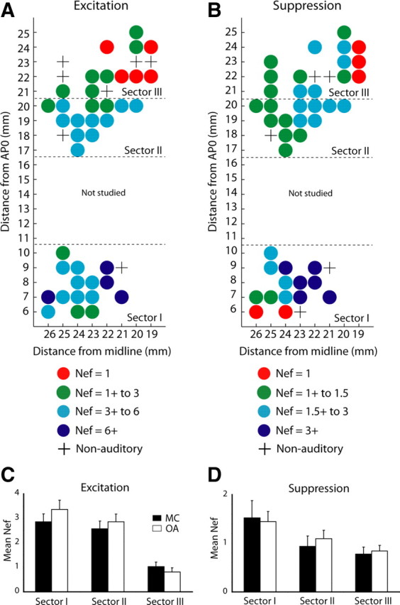
A, B, Distribution along the STP of the Nef per neuron yielding excitation and suppression, respectively. The Nef was calculated for each auditory responsive neuron that showed an excitation response and/or suppression response, and the mean Nef (for both monkeys) was mapped on the recording sites, collapsed across depth, on the 1 × 1 mm grid. The data were smoothed by using a moving average (boxcar filter, 3 × 3 mm) ignoring the empty (nonauditory) coordinates marked with a “+.” x-axis, Millimeters lateral to midline; y-axis, millimeters anterior to AP0. Nef is color-coded. It should be noted that the caudolateral recording sites in sector I may have extended beyond the lateral border of area A1 into the lateral belt (Morel et al., 1993; Hackett et al., 1998), and this could have contributed to the increased responsiveness of these particular sites to different stimulus types. C, D, Mean Nef (±SE) for each of the three sectors, plotted separately for MC and OA sounds. C, Excitation, Nef in sector III is lower than Nef in both sectors II and I at p < 0.02 for MC stimuli and p < 0.01 for OA stimuli. D, Suppression, Nef in sector III is lower than Nef in sector I at p < 0.05 for OA stimuli (see text for additional details). Note the following: (1) change in color code between A and B; (2) change in ordinate scale between C and D; and (3) Nef values per sector quoted in the text for 40 S− sounds are the sum of the separate Nefs for MC and OA, which include 20 S− sounds each.

The same analysis as that described above for excitation responses was performed for suppression responses (Table 1; supplemental Fig. 5, available at www.jneurosci.org as supplemental material). The Nef for suppression responses also decreased progressively as the site moved rostrally (Fig. 6B): sector 1, 2.97 ± 0.51 (mean ± SEM), N = 65; sector II, 2.03 ± 0.35, N = 64; sector III, 1.62 ± 0.22, N = 63. A two-way, repeated-measures ANOVA again showed a main effect of recording site (F_(2,189) = 3.33; p < 0.05) and not of stimulus category or of their interaction (Fig. 6D); here, the post hoc paired comparisons yielded a significantly lower Nef in sector III than in sector I for OA stimuli (p < 0.05).

Adoption of a more liberal criterion for the definition of an excitation response by reducing the number of SDs above baseline firing rate from 2.8 (p < 0.005) to 2.5 or 2.0 SDs above baseline (values of p < 0.012 and 0.046, respectively) increased the mean Nef substantially (supplemental Fig. 6, available at www.jneurosci.org as supplemental material), but the change affected the Nef in all three sectors proportionately and so had no significant effect on the differences between them.

Interestingly, the increase in stimulus selectivity of both excitation and suppression responses as the recordings moved rostrally occurred despite the opposite trends in prevalence of the two response types (i.e., the disproportionate caudal-to-rostral decrease in excitation-only responses and disproportionate caudal-to-rostral increase in suppression-only responses). Thus, degree of stimulus selectivity within a particular response type and prevalence of that response type appeared to vary independently of each other. On a proportional basis, the ratio of Nef for suppression to Nef for excitation was more than seven times greater in sector III (1.79) than in the other two sectors (0.24 in each).

To examine the relationship between stimulus selectivity and response type more closely, we performed three-way, repeated-measures ANOVA by adding the factor of response type to the two-way ANOVAs described above. This analysis revealed that stimulus selectivity varied strongly not only with recording site (F_(2,445) = 8.82; p < 0.001) but also with response type (F_(1,445) = 18.68; p < 0.001) and, furthermore, that there was an interaction between the two factors (F_(2,445) = 3.07; p < 0.05). This interaction, reflecting a selective, precipitous drop in the Nef for excitation between sectors II and III, is illustrated in supplemental Figure 7 (available at www.jneurosci.org as supplemental material).

Response latencies

Onset latencies of the excitation responses increased progressively as the recordings proceeded rostrally (Fig. 7) (medians and SEs for sectors I–III: 58 ± 2.2, 72 ± 2.3, and 112 ± 9.4 ms, respectively; Kruskal–Wallis test, p < 0.05), and all three pairwise differences were significant (values of p < 0.05, Kolmogorov–Smirnov test). Similar results were obtained for minimum latencies (medians and SEs for sectors I–III: 37 ± 4.7, 43 ± 5.0, 74 ± 11.0 ms, respectively; Kruskal–Wallis test, p < 0.05), although in this case the increase was significant only between each of the first two sectors and sector III (both values of p < 0.01, Kolmogorov–Smirnov test).

Figure 7.

Response latencies across the three sectors. Median (±SE) minimum latencies (dark gray bars) and onset latencies (light gray bars). All pairwise comparisons across sectors are significant (values of p ranging from 0.05 to 0.01, except for the difference in onset latency between sectors I and II).

Because the 40 S− stimuli varied so widely in their sound envelopes and other spectrotemporal features, the above latency differences among the three sectors could have been attributable simply to differences in their sound preferences. We therefore performed a separate analysis comparing the minimum latencies of neurons in the different sectors to the three pure tones only (see Materials and Methods). However, because sector III neurons in particular tended to respond to complex acoustic stimuli rather than to the pure tones (supplemental Fig. 5, available at www.jneurosci.org as supplemental material), we collapsed the sample sizes from sectors II and III (27 and 3 cells, respectively) to form an rSTP group (30 cells) for comparison with sector I (mostly area A1, 37 cells). The comparison confirmed that median minimum response latencies (A1, 42 ms; rSTP, 85 ms) differed significantly (p < 0.05, Kolmogorov–Smirnov test), in this case to the same three pure tones.

Response magnitudes

For the reason spelled out above concerning the unequal number of neurons in the three sectors (see above, Response latencies), we collapsed the firing-rate data from sectors II and III to form an rSTP group (131 neurons) for comparison with sector I (area A1, 128 neurons). As illustrated in Figure 8A, the firing rates to both MC and OA stimuli for the entire duration of the stimuli averaged ∼3 spikes/s above baseline, with one exception. For OA stimuli in sector I, the mean response magnitude rose to nearly twice that rate (i.e., close to 6 spikes/s above baseline). A two-way ANOVA indicated that there was a main effect of recording site (F_(1,1394) = 23.4; p < 0.001) and stimulus category (F_(1,1394) = 8.51; p < 0.01), as well as a significant interaction between them (F_(1,1394) = 13.9; p < 0.001). The mean response magnitude for OA stimuli in A1 was significantly greater than that for both MC stimuli in A1 and OA stimuli in rSTP (Wilcoxon's rank sum test: MC in A1 vs OA in A1, p < 10⁻³; OA in A1 vs OA in rSTP, p < 10⁻⁴).

Figure 8.

A, Mean response magnitudes (±SE) in A1 and rSTP for MC stimuli (black bars) and OA stimuli (white bars). B, Mean peak response magnitudes for two different time windows: 50 and 100 ms (i.e., 25 and 50 ms, respectively, on either side of the peak latency) and for the entire duration of each sound. C, Mean peak response magnitudes; otherwise, same as A. D, Distribution of mean response magnitudes per stimulus for all auditory responses in A1 and rSTP. Note that, in A1, the two most effective stimuli were the pure tones, 5 and 10 kHz (sounds 39 and 40, respectively), marked by arrows. E, Distribution of mean peak response magnitudes per stimulus for all auditory responses in A1 and rSTP; otherwise same as D. Note also change in ordinate scales between A and C and also between D and E.

The same results as those obtained for mean response magnitudes across the full stimulus duration were also observed for peak response magnitudes, independent of the size of the response window (Fig. 8B). Thus, for both the 50 and 100 ms windows, significant effects were obtained for recording site (F_(1,1394) = 55.9 and 37.3, respectively; values of p < 0.001), stimulus category (F_(1,1394) = 14.3 and 15.0, respectively; values of p < 0.001), and the interaction of those two factors (F_(1,1394) = 20.6 and 21.9, respectively; values of p < 0.001). These results are illustrated for 50 ms windows in Figure 8C.

We also examined the distribution of the response magnitudes per stimulus (Fig. 8D,E) and found that, among all 40 of the S− sounds we used, the two most effective ones in A1 were the 5 and 10 kHz pure tones (mean rates of 11.9 and 9.1 spikes/s, respectively; and peak rates of 24.2 and 26.3 spikes/s, respectively).

Discussion

We compared the auditory response properties of 362 neurons distributed among three different sectors, I–III, located primarily within auditory areas A1, RT, and RTp, respectively, while the animals listened attentively to 20 MCs and 20 OA stimuli. The results provide evidence in favor of the hypothesis that the three different sectors form part of a rostrally directed stimulus quality processing stream.

Rostrally directed stimulus quality pathway originating in A1

Neurons across the three sectors differed significantly in the mean Nef to which they gave either excitation or suppression responses, showing increasing stimulus selectivity for both types of response as the recordings moved rostrally along the STP. Across the three sectors, the mean Nef for excitation dropped from a value representing 16% of the total number of S− sounds we used to one representing 5%, and the corresponding mean Nef values for suppression dropped from 7 to 4%. Both decreases, each of which was significant, were approximately the same for MC and OA stimuli. It should be noted that the caudal-to-rostral decreases in Nef for both excitation and suppression were accompanied by a substantial caudal-to-rostral increase in the proportion of neurons showing “suppression-only” responses. The latter trend toward increasing suppression could well be partly responsible for the former trend toward greater stimulus selectivity.

The gradient increase in stimulus selectivity from the primary auditory area to rSTP was paralleled by a gradient increase in response latency across the three auditory subdivisions. The minimum latency of neurons with excitation responses increased significantly as the recordings proceeded rostrally (sectors I–III: 37, 43, and 74 ms, respectively). The average minimum response latency to pure tones in sector I is similar to the value reported for area A1 in one study [40 ms (Remedios et al., 2009)], although much shorter A1 latencies have also been observed [27 ms (Bendor and Wang, 2008); 12–20 ms (Kuśmierek and Rauschecker, 2009)]. The extremely short latencies in the latter studies presumably reflected the use of tonal stimuli at the best frequency and loudness for evoking a response from tonotopically organized A1. However, despite the use of stimuli in the present study that yielded relatively long response latencies in A1, it is clear that the latencies to the same stimuli in rSTP were even longer. Although the ventral division of the medial geniculate nucleus sends direct projections to all auditory core areas (Jones, 2003), these areas are also interconnected by corticocortical projections (Morel et al., 1993; Kaas and Hackett, 2000), providing a potential basis for stepwise serial processing with increasing response latencies as information proceeds rostrally out of A1. Such a serial processing pathway would allow for the gradually increasing stimulus selectivity from early to later stations of the kind observed in this study, paralleling that observed in the ventral processing pathway for object vision.

Our results also showed that both mean and peak response magnitudes for the OA stimuli were especially high in sector I and then dropped sharply in sectors II and III. The high firing rates to OA stimuli in sector I are consistent with the notion that the great majority of A1 neurons are tuned to relatively simple acoustic features (specific frequency, spectral-band size, clicks, etc.), including two different tone pips (Sadagopan and Wang, 2009), and so respond at high rates to simple stimuli limited to just these features or to complex stimuli that contain these features (supplemental Fig. 1, available at www.jneurosci.org as supplemental material). If this interpretation is correct, then the selective decrease in the responsivity of rSTP neurons to OA stimuli implies that the majority of these cells, unlike those in area A1, are driven best by complex acoustic features rather than simple ones. This interpretation has been used as a central hypothesis in a computational neural network model of auditory object processing (Husain et al., 2004). Moreover, as a result of the selective decrease in the firing rates of rSTP neurons to OA stimuli, the excitation responses elicited by monkey calls represented approximately one-half of all the activity evoked in this region by the 40 stimuli we used, whereas in A1 they represented only approximately one-third of the total activity evoked by the same 40 stimuli. Indeed, some rSTP neurons showed an absolute increase in responsivity to monkey calls (Fig. 4), firing to fully one-half of the MC stimuli at rates higher than those to all but one or two OA stimuli. These findings on response latency and response magnitude, together with the increased stimulus selectivity of rSTP neurons, all imply that rSTP is at a higher level of auditory processing than area A1.

The results summarized above are thus in line with the proposal that the supratemporal plane is the site of an auditory processing stream composed of a series of cortical re-representations of cochlear tonotopy—areas A1, R, and RT—with an extension into a potentially nontonotopic representation—area RTp. Such an organization would closely resemble that of the ventral visual pathway, which is likewise composed of a series of cortical re-representations of the sensory surface (i.e., the retinotopically organized areas V1 thru TEO, with an extension into a nonretinotopic representation, area TE). Also like the ventral visual pathway, the supratemporal auditory pathway could be dedicated to representing complex stimuli as neuronal ensembles [cf. the network model of Husain et al. (2004)], which could then enter into a wide variety of stimulus–stimulus, stimulus–response, and stimulus–emotional state associations through the connections of this pathway to cortical polysensory, neostriatal, and limbic circuits, respectively. Among the many categories of complex stimuli for which this auditory pathway could be critical are not only monkey vocalizations (Poremba et al., 2004) but also the individual voices of conspecifics, as suggested by the studies of Petkov et al. (2008, 2009). Indeed, the monkey's vocalization and voice area that these investigators identified with neuroimaging methods is located in rSTP.

Two directions of information flow within the superior temporal gyrus

The evidence reported here for the existence of a rostrally directed, stimulus quality pathway originating in A1 does not imply that every auditory dimension or property important for representing stimulus quality is processed via this route. On the contrary, some acoustic properties must use the well established route that proceeds laterally from core to belt to parabelt. For example, one acoustic dimension that seems to engage this laterally directed pathway and not the rostrally directed one is sound intensity. A recent neuroimaging study (Tanji et al., 2009) found that the reversals of tonotopic representation that define the borders between A1 and R and between R and RT were present at all sound levels tested, whereas there was increasing spread of activation into the adjacent lateral and posteromedial belt areas as the amplitude of the pure tones was increased. This finding is consistent with evidence from microelectrode recording in monkeys (Kosaki et al., 1997; Recanzone et al., 2000) indicating that belt area neurons have higher intensity thresholds for pure tones than do neurons in the auditory core.

Whether other properties of acoustic stimuli also selectively engage the laterally as opposed to the rostrally directed pathway is presently unclear. Two candidates are narrow-band noise and frequency-modulated sweeps, which, as indicated previously, stimulate auditory belt neurons more effectively than pure tones do (Rauschecker and Tian, 2004; Tian and Rauschecker, 2004). However, monkey calls also activate auditory belt neurons better than do pure tones (Tian et al., 2001), indicating that identification of those acoustic features and stimulus categories that evoke activity selectively, or preferentially, in one of the two orthogonally oriented pathways can only be determined by direct comparison of the responsivity of these two pathways to each type of acoustic stimulus of interest.

The same is true for the interesting possibility suggested by Bendor and Wang (2008) that the two pathways divide spectrotemporal processing into its two domains, spectral and temporal. One basis for such a division of labor is the evidence that the spectral (i.e., tonal-frequency) integration windows of single cells become progressively larger as one proceeds from core to belt to parabelt, possibly rendering the parabelt neurons particularly well suited for discriminating not only the size of spectral bandwidths but also complex spectral shapes. The second basis for this potential functional division is new evidence gathered by Bendor and Wang (2008) that a subset of neurons in the auditory core areas of the marmoset shows peak firing rates that shift progressively to higher temporal frequencies of amplitude-modulated sounds as the recordings move from A1 to R to RT. Based on this finding, the authors proposed that temporal integration windows increase rostrally, thereby rendering the rostral core areas better suited than area A1 for discriminating the temporal features of acoustic stimuli. If, as now seems likely, there are indeed two different directions of information flow within the superior temporal gyrus, one rostrally directed, the other laterally directed, then exactly what type of auditory stimulus quality information each route specializes in processing—spectral versus temporal or any other functional division—is open to direct test. We suspect that subjecting such comparisons to direct test will soon become an important research endeavor, as it promises to greatly improve our understanding of how complex auditory stimuli are encoded.

References

- Bendor D, Wang X. Neural response properties of primary, rostral, and rostrotemporal core fields in the auditory cortex of marmoset monkeys. J Neurophysiol. 2008;100:888–906. doi: 10.1152/jn.00884.2007. [DOI] [PMC free article] [PubMed] [Google Scholar]
- Cohen YE, Russ BE, Gifford GW, 3rd, Kiringoda R, MacLean KA. Selectivity for the spatial and nonspatial attributes of auditory stimuli in the ventrolateral prefrontal cortex. J Neurosci. 2004;24:11307–11316. doi: 10.1523/JNEUROSCI.3935-04.2004. [DOI] [PMC free article] [PubMed] [Google Scholar]
- de la Mothe LA, Blumell S, Kajikawa Y, Hackett TA. Cortical connections of the auditory cortex in marmoset monkeys: core and medial belt regions. J Comp Neurol. 2006;496:27–71. doi: 10.1002/cne.20923. [DOI] [PubMed] [Google Scholar]
- Fitzpatrick KA, Imig TJ. Auditory cortico-cortical connections in the owl monkey. J Comp Neurol. 1980;192:589–610. doi: 10.1002/cne.901920314. [DOI] [PubMed] [Google Scholar]
- Fritz J, Mishkin M, Saunders RC. In search of an auditory engram. Proc Natl Acad Sci U S A. 2005;102:9359–9364. doi: 10.1073/pnas.0503998102. [DOI] [PMC free article] [PubMed] [Google Scholar]
- Galaburda AM, Pandya DN. The intrinsic architectonic and connectional organization of the superior temporal region of the rhesus monkey. J Comp Neurol. 1983;221:169–184. doi: 10.1002/cne.902210206. [DOI] [PubMed] [Google Scholar]
- Gifford GW, 3rd, MacLean KA, Hauser MD, Cohen YE. The neurophysiology of functionally meaningful categories: macaque ventrolateral prefrontal cortex plays a critical role in spontaneous categorization of species-specific vocalizations. J Cogn Neurosci. 2005;17:1471–1482. doi: 10.1162/0898929054985464. [DOI] [PubMed] [Google Scholar]
- Hackett TA, Stepniewska I, Kaas JH. Subdivisions of auditory cortex and ipsilateral cortical connections of the parabelt auditory cortex in macaque monkeys. J Comp Neurol. 1998;394:475–495. doi: 10.1002/(sici)1096-9861(19980518)394:4<475::aid-cne6>3.0.co;2-z. [DOI] [PubMed] [Google Scholar]
- Hackett TA, Stepniewska I, Kaas JH. Prefrontal connections of the parabelt auditory cortex in macaque monkeys. Brain Res. 1999;817:45–58. doi: 10.1016/s0006-8993(98)01182-2. [DOI] [PubMed] [Google Scholar]
- Husain FT, Tagamets MA, Fromm SJ, Braun AR, Horwitz B. Relating neuronal dynamics for auditory object processing to neuroimaging activity: a computational modeling and an fMRI study. Neuroimage. 2004;21:1701–1720. doi: 10.1016/j.neuroimage.2003.11.012. [DOI] [PubMed] [Google Scholar]
- Jones EG. Chemically defined parallel pathways in the monkey auditory system. Ann N Y Acad Sci. 2003;999:218–233. doi: 10.1196/annals.1284.033. [DOI] [PubMed] [Google Scholar]
- Kaas JH, Hackett TA. Subdivisions of auditory cortex and processing streams in primates. Proc Natl Acad Sci U S A. 2000;97:11793–11799. doi: 10.1073/pnas.97.22.11793. [DOI] [PMC free article] [PubMed] [Google Scholar]
- Kosaki H, Hashikawa T, He J, Jones EG. Tonotopic organization of auditory cortical fields delineate by parvalbumin immunoreactivity in macaque monkeys. J Comp Neurol. 1997;386:304–316. [PubMed] [Google Scholar]
- Kuśmierek P, Rauschecker JP. Functional specialization of medial auditory belt cortex in the alert rhesus monkey. J Neurophysiol. 2009;102:1606–1622. doi: 10.1152/jn.00167.2009. [DOI] [PMC free article] [PubMed] [Google Scholar]
- Morel A, Garraghty PE, Kaas JH. Tonotopic organization, architectonic fields, and connections of auditory cortex in macaque monkeys. J Comp Neurol. 1993;335:437–459. doi: 10.1002/cne.903350312. [DOI] [PubMed] [Google Scholar]
- Petkov CI, Kayser C, Steudel T, Whittingstall K, Augath M, Logothetis NK. A voice region in the monkey brain. Nat Neurosci. 2008;11:367–374. doi: 10.1038/nn2043. [DOI] [PubMed] [Google Scholar]
- Petkov CI, Logothetis NK, Obleser J. Where are the human speech and voice regions, and do other animals have anything like them? Neuroscientist. 2009;15:419–429. doi: 10.1177/1073858408326430. [DOI] [PubMed] [Google Scholar]
- Petrides M, Pandya DN. Association fiber pathways to the frontal cortex from the superior temporal region in the rhesus monkey. J Comp Neurol. 1988;273:52–66. doi: 10.1002/cne.902730106. [DOI] [PubMed] [Google Scholar]
- Poremba A, Mishkin M. Exploring the extent and function of higher-order auditory cortex in rhesus monkeys. Hear Res. 2007;229:14–23. doi: 10.1016/j.heares.2007.01.003. [DOI] [PMC free article] [PubMed] [Google Scholar]
- Poremba A, Malloy M, Saunders RC, Carson RE, Herscovitch P, Mishkin M. Species-specific calls evoke asymmetric activity in the monkey's temporal poles. Nature. 2004;427:448–451. doi: 10.1038/nature02268. [DOI] [PubMed] [Google Scholar]
- Rauschecker JP, Tian B. Mechanisms and streams for processing of “what” and “where” in auditory cortex. Proc Natl Acad Sci U S A. 2000;97:11800–11806. doi: 10.1073/pnas.97.22.11800. [DOI] [PMC free article] [PubMed] [Google Scholar]
- Rauschecker JP, Tian B. Processing of band-passed noise in the lateral auditory belt cortex of the rhesus monkey. J Neurophysiol. 2004;91:2578–2589. doi: 10.1152/jn.00834.2003. [DOI] [PubMed] [Google Scholar]
- Rauschecker JP, Tian B, Hauser M. Processing of complex sounds in the macaque nonprimary auditory cortex. Science. 1995;268:111–114. doi: 10.1126/science.7701330. [DOI] [PubMed] [Google Scholar]
- Recanzone GH, Guard DC, Phan ML. Frequency and intensity response properties of single neurons in the auditory cortex of the behaving macaque monkey. J Neurophysiol. 2000;83:2315–2331. doi: 10.1152/jn.2000.83.4.2315. [DOI] [PubMed] [Google Scholar]
- Remedios R, Logothetis NK, Kayser C. An auditory region in the primate insular cortex responding preferentially to vocal communication sounds. J Neurosci. 2009;29:1034–1045. doi: 10.1523/JNEUROSCI.4089-08.2009. [DOI] [PMC free article] [PubMed] [Google Scholar]
- Romanski LM, Goldman-Rakic PS. An auditory domain in primate prefrontal cortex. Nat Neurosci. 2002;5:15–16. doi: 10.1038/nn781. [DOI] [PMC free article] [PubMed] [Google Scholar]
- Romanski LM, Bates JF, Goldman-Rakic PS. Auditory belt and parabelt projections to the prefrontal cortex in the rhesus monkey. J Comp Neurol. 1999a;403:141–157. doi: 10.1002/(sici)1096-9861(19990111)403:2<141::aid-cne1>3.0.co;2-v. [DOI] [PubMed] [Google Scholar]
- Romanski LM, Tian B, Fritz J, Mishkin M, Goldman-Rakic PS, Rauschecker JP. Dual streams of auditory afferents target multiple domains in the primate prefrontal cortex. Nat Neurosci. 1999b;2:1131–1136. doi: 10.1038/16056. [DOI] [PMC free article] [PubMed] [Google Scholar]
- Romanski LM, Averbeck BB, Diltz M. Neural representation of vocalizations in the primate ventrolateral prefrontal cortex. J Neurophysiol. 2005;93:734–747. doi: 10.1152/jn.00675.2004. [DOI] [PubMed] [Google Scholar]
- Russ BE, Ackelson AL, Baker AE, Cohen YE. Coding of auditory-stimulus identity in the auditory non-spatial processing stream. J Neurophysiol. 2008;99:87–95. doi: 10.1152/jn.01069.2007. [DOI] [PMC free article] [PubMed] [Google Scholar]
- Sadagopan S, Wang X. Nonlinear spectrotemporal interactions underlying selectivity for complex sounds in auditory cortex. J Neurosci. 2009;29:11192–11202. doi: 10.1523/JNEUROSCI.1286-09.2009. [DOI] [PMC free article] [PubMed] [Google Scholar]
- Saleem KS, Logothetis NK. A combined MRI and histology atlas of the rhesus monkey brain. London: Academic; 2007. [Google Scholar]
- Strominger NL, Oesterreich RE, Neff WD. Sequential auditory and visual discriminations after temporal lobe ablation in monkeys. Physiol Behav. 1980;24:1149–1156. doi: 10.1016/0031-9384(80)90062-1. [DOI] [PubMed] [Google Scholar]
- Tanji K, Leopold DA, Ye FQ, Zhu C, Malloy M, Saunders RC, Mishkin M. Effect of sound intensity on tonotopic fMRI maps in the unanesthetized monkey. Neuroimage. 2009;49:150–172. doi: 10.1016/j.neuroimage.2009.07.029. [DOI] [PMC free article] [PubMed] [Google Scholar]
- Tian B, Rauschecker JP. Processing of frequency-modulated sounds in the lateral auditory belt cortex of the rhesus monkey. J Neurophysiol. 2004;92:2993–3013. doi: 10.1152/jn.00472.2003. [DOI] [PubMed] [Google Scholar]
- Tian B, Reser D, Durham A, Kustov A, Rauschecker JP. Functional specialization in rhesus monkey auditory cortex. Science. 2001;292:290–293. doi: 10.1126/science.1058911. [DOI] [PubMed] [Google Scholar]