

Abstract
To improve the prediction accuracy in the regime where template alignment quality is poor, an updated version of TASSER_2.0, namely TASSER_WT, was developed. TASSER_WT incorporates more accurate contact restraints from a new method, COMBCON. COMBCON uses confidence-weighted contacts from PROSPECTOR_3.5, the latest version, PROSPECTOR_4, and a new local structural fragment-based threading algorithm, STITCH, implemented in two variants depending on expected fragment prediction accuracy. TASSER_WT is tested on 622 Hard proteins, the most difficult targets (incorrect alignments and/or templates and incorrect side-chain contact restraints) in a comprehensive benchmark of 2591 nonhomologous, single domain proteins ≤200 residues that cover the PDB at 35% pairwise sequence identity. For 454 of 622 Hard targets, COMBCON provides contact restraints with higher accuracy and number of contacts per residue. As contact coverage with confidence weight ≥3 (Fwt≥3cov) increases, the more improved are TASSER_WT models. When Fwt≥3cov > 1.0 and > 0.4, the average root mean-square deviation of TASSER_WT (TASSER_2.0) models is 4.11 Å (6.72 Å) and 5.03 Å (6.40 Å), respectively. Regarding a structure prediction as successful when a model has a TM-score to the native structure ≥0.4, when Fwt≥3cov > 1.0 and > 0.4, the success rate of TASSER_WT (TASSER_2.0) is 98.8% (76.2%) and 93.7% (81.1%), respectively.
Introduction
Owing to intensive effort over the last several decades, the accuracy of protein structure prediction methods has seen continual improvement (1–6). There are two basic approaches to the prediction of protein structure: those that are structural template-based (TB), and those that do not use any preexisting structural information, i.e., template-free (TF) (2,4,6–9). Both comparative modeling and threading are based on the same strategy that identifies a set of templates that have related structures to the target sequence. Although comparative modeling mainly relies on evolutionary relationships between the target and template, in principle, threading aims to identify target-template pairs that adopt similar structures whether or not they are evolutionary related (10). However, in practice, the best threading methods have a strong evolutionary component and purely structure-based approaches have not been competitive (11,12). For single domain proteins, TB methods can identify structurally related templates for ∼75% of sequences in an average proteome (13). However, given that the Protein DataBank (PDB) is likely complete for single domain proteins, it fails for the remaining 25% of targets either because structurally similar templates are either evolutionarily unrelated or because they are far too distant to be detected with accurate alignments (14). On the other hand, TF methods predict the tertiary structure of the target protein simply from protein sequence without any extrinsic structural information. Conceptually, TF methods are the most elegant, but their accuracy is on average much worse than TB approaches (15).
The reason that TB methods are the most successful structure prediction approaches is due to the improvement in fold recognition algorithms (16,17) and the increased number of solved protein structures in the Protein DataBank (PDB) (18). However, for those target proteins that are weakly (distantly related)/nonhomologous to proteins in the PDB, TB methods often perform quite poorly (13). Recent developments of the TASSER protein structure prediction algorithm and its variants (among the top-ranked algorithms in CASP8 (13,14,19–25)) have shown some progress for these difficult targets. Although TASSER can operate in the TF limit with moderate success (24,26), it is the most effective when it incorporates template alignments and side chain contact restraints from threading (e.g., from PROSPECTOR_3.5) for refining the structures (13,14). Therefore, the performance of TASSER is dependent on the accuracy and coverage of predicted contact restraints.
The next generation of TASSER, TASSER_2.0 (14) provided for improved contact prediction accuracy on a comprehensive, large-scale benchmark test set consisting of 2,591 nonhomologous, single domain proteins having ≤ 200 residues. Based on their threading score significance, target proteins are categorized into Easy (1802 targets) with accurate template identification/alignments, Medium (167 targets), templates with good structural alignments but poor threading alignments, and Hard (622 targets) with acceptable structural alignments at low coverage but on average poor threading alignment accuracy. This classification indicates the relative confidence in the prediction accuracy. The accuracy of predicted side-chain contact restraints as well as template alignments are dependent on target difficulty. In the benchmark set, the average contact prediction accuracy (number of correctly predicted contacts divided by the number of contacts predicted; strictly speaking, this is the contact prediction precision) improved from 0.37 using wild-type sequences in PROSPECTOR_3.5 to 0.60 (with an average number of contacts/residue of 1.34) (13) in TASSER_2.0. Hard targets have an average side-chain contact prediction accuracy of 0.50, but the coverage is low, with 0.25 contacts/residue on average. Because of the small number of correctly predicted contacts, TASSER_2.0 fails to generate reasonably accurate models for many Hard targets (14). Therefore, improvement in prediction accuracy for Hard targets is needed.
In this work, as part of our ongoing efforts to improve the accuracy of the predicted side chain contact restraints, we develop a new (to our knowledge) approach for template identification/contact prediction. In addition to using wild-type template sequences in PROSPECTOR_3.5, we develop an improved threading algorithm PROSPECTOR_4 that differs from previous generations of PROSPECTOR (14,27,28) in a number of important respects: For the sequence profile component of the scoring function, for an 11-residue window centered at each target residue i and template residue j, we calculate the average sequence profile score. Given that score and the alignment (i−5,j−5), …(i+5,j+5), we calculate the probability that at least 50% of these aligned pairs correspond to the best structure alignment as provided by fr-TM-align (29). The second pass uses the alignment generated in the first pass to evaluate the partners used to the calculation of the pair interactions, also averaged over an 11-residue window. As shown below, compared to PROSPECTOR_3.5, PROSPECTOR_4 provides an ∼3% higher TM-score. We next use the top five templates selected by PROSPECTOR_4 as structural splines in a newly developed fragment-stitching algorithm, STITCH. STITCH takes advantage of the fact that for even for Hard targets, ∼77% of PROSPECTOR_4 identified templates have good structural alignments to the target's native structure, even though the sequence alignments are of moderate to poor accuracy. Two local fragment scores provide two sets of target-template alignments. In the prediction of tertiary contacts, we combine all four approaches to provide a set of weighted contact predictions whose weight is strongly correlated with contact prediction accuracy; we term this composite approach, COMBCON. The predicted contacts plus the template alignments provided by PROSPECTOR_4 are implemented into a new structure refinement approach, TASSER_WT. We benchmarked TASSER_WT on the 622 Hard targets of our previous comprehensive benchmark test set (14) and provide a detailed comparison with the previous TASSER_2.0 predictions. Significant improvement of TASSER_WT for the majority of difficult, Hard set of targets is demonstrated.
Materials and Methods
Overview
TASSER and its variants are basically composed of template identification and side chain and contact restraint prediction by threading, followed by structure assembly and final model selection. As shown in the flow chart of the methodology, in Fig. 1, after running the various threading algorithms, we combine the side chain contacts predicted by PROSPECTOR_3.5, PROSPECTOR_4, and SPLINE_high/low, with the weight of a predicted contact between side chains i and j, wt(i,j), given by the number of times it is found in the four approaches. TASSER_WT uses the modified additional contact restraint energy function previously developed in TASSER_2.0 to increase the influence of more accurately predicted contacts as well as the template alignments provided from PROSPECTOR_4 as input. Because the same procedures for structure assembly and final model selection are used by TASSER_2.0 and TASSER_WT (13,14,30), we focus on the newly developed PROSPECTOR_4 and SPLINE_high/low methods and the modified contact restraint energy.
Figure 1.
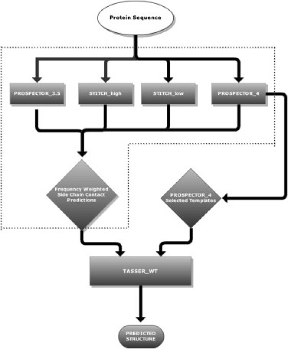
Flow chart of the COMBCON and TASSER_WT algorithms. The COMBCON algorithm is delineated by the dashed lines. A given protein sequence is subject to the four threading algorithms, PROSPECTOR_3.5, PROSPECTOR_4, STITCH_high, and STITCH_low, and the resulting set of contacts are weighted by the total frequency of occurrence in the four methods. These frequency-weighted contacts are then provided to the TASSER_WT structure assembly algorithm along with the set of PROSPECTOR_4-provided template alignments.
PROSPECTOR_3.5
In what follows, we use the template wild-type sequences and their associated sequence profiles of PROSPECTOR_3.5, as described in Lee and Skolnick (14). From the final iteration of PROSPECTOR_3.5, a pair of residues (>4 residues apart in sequence) are predicted to be in contact if in the up to 30 scoring templates as ranked by their z-score ≥4, the following conditions hold: For those contacts occurring in at least three of the templates (assigned a weight of unity each time it occurs), the weight of all aligned contacts within ±3 residues of a contact is increased by 1 if the BLOSUM62 (31) matrix elements of the two target/template pairs of aligned residues are >0. If the resulting contact weight >4, the pair is predicted to be in contact.
PROSPECTOR_4
PROSPECTOR_4 incorporates many of the ideas of PROSPECTOR_3.5 (14), but gives improved accuracy at roughly 60% of the computational cost due to the decreased number of iterations required to achieve convergence. For the e10 sequence profiles (those sequences whose PSIBLAST (32) E-value to the target or template sequence is ≤10) of the target (template) of length M (N), let xi (Xi) be a 20-dimensional vector, the lth element of which is the frequency of occurrence of amino acid type α (α = 1,2,…..,20) at position i. We then calculate the corresponding z-score (score in standard deviation units relative to the mean) of the target and template residues i and j of type α as
| (1a) |
| (1b) |
where σκ is the standard deviation in amino-acid frequency and 〈…〉 is the average value (0.05) at position κ. The (i,j) matrix element of the score associated with aligning target residue i to template residue j is related to the probability p1/2 that a window of ℓ ((= 2ω+1) = 11) residues centered at i with average correlation coefficient
| (2) |
have a best structural alignment to the native structure (which is of course unknown at the time of the alignment because no knowledge of the native structure is used) for at least 50% of the residues by
| (3) |
(The list of nonhomologous training proteins used to derive this is found at http://cssb.biology.gatech.edu/skolnick/files/TASSER_WT/LIST.train.) The value p1/2 for a given score is given in Table 1, where we use a set of discretized values. The correlation coefficient between the fraction of residues in the window that correspond to the best structural alignment and is 0.71. We use a = 0.19, b = 0.2 with gap creation and propagation penalties of −2.15 and −0.16. Values a and b were obtained by optimizing the accuracy of the threading alignments on the first 99 proteins found in LIST.train.
Table 1.
Probability that a given correlation coefficient over an 11- residue window has at least half of its residues corresponding to the best target-template structural alignment
| Correlation coefficient, Cb | p1/2 |
|---|---|
| <0 | 0.0 |
| 0.0 | 0.097 |
| 0.1 | 0.142 |
| 0.2 | 0.219 |
| 0.3 | 0.344 |
| 0.4 | 0.506 |
| 0.5 | 0.694 |
| 0.6 | 0.818 |
| 0.7 | 0.88 |
| 0.8 | 0.898 |
| 0.9 | 0.909 |
| 1.0 | 0.918 |
Let M1(j) be the alignment of template residue j to target residue i given by the first pass of threading using Eq. 3. We then use this target/template structure alignment to identify the partners for the evaluation of the pair interactions in the second pass of threading as
| (4) |
where ɛpair is the sum of the target protein's multiple sequence averaged, protein-specific pair potential and our previously derived quasichemical pair potential (33). In practice, for template ranking, we calculate the z-score of the difference between the target-template score and that when the target sequence is reversed; the latter is designed to remove composition dependences of the scoring function. (The quasichemical pair potential may be found at http://cssb.biology.gatech.edu/skolnick/files/TASSER_WT/quasichemical_pair .)
In PROSPECTOR_4, template rankings and alignments are taken from the second pass of threading. For the top-ranked, up to 30 templates, all having a z-score > 1.75, we set the weight of a contact that is equal to 1, if the z-score < 20; otherwise, the weight = 3. We then sum the weights over all the examined templates. As in PROSPECTOR_3.5, we follow the identical procedure to augment the weights of the contacts with favorable BLOSUM62 mutation matrix elements. A pair of residues are then predicted to be in contact if the weight of the contacts constructed by the aforementioned procedure >1.
STITCH fragment assembly algorithm
Fragment selection
As shown below, for ∼77% of Hard targets, even when PROSPECTOR_4 fails to generate a good threading alignment, the templates have a good structural alignment to native. As will be shown elsewhere (J. Skolnick and M. Brylinski, unpublished), the reason these templates are selected is that they often retain the ancestral functional site of the target, but have diverged to the point that the sequence profile component of Eq. 3 is too weak to generate a good alignment. The idea of the STITCH algorithm is to identify 13-residue local fragments that are then aligned to the template structure and combined or stitched together to generate a global alignment. The template is then used to position the overlapping fragments whose average coordinates constitute the alignment. The template also provides a subset of predicted contacts used in the contact-weighting procedure described below.
The set of the top, up to 30, PROSPECTOR_4 templates whose z-score ≥ 4 provides the structures from which the fragments are extracted. We consider ℓ= 13 residue fragments. For target residue i, the score of the template fragment centered at residue j, Efrag(i,j), is given by a combination of the sequence covariation term, Eq. 2 with ω = 6, the fraction of residues in the fragment where the template's secondary structure agrees with the predicted target secondary structure (14), fsec(i,j), a sequence profile averaged, backbone dihedral angle potential, ɛdih(i,j) and a target sequence profile averaged side-chain contact number potential, ɛcon(i,j). Based on optimization over the training set, we take
| (5a) |
In Eq. 5a, we use the predicted secondary structure from the neural network described in Lee and Skolnick (14) and averaged over ℓ; namely,
| (5b) |
where δi+Δ, j+Δ = 1 when the predicted secondary structure of residue i+Δ is the same as that of template residue j+Δ; it is zero, otherwise. Next, we consider the sequence-profile-averaged, dihedral angle potential
| (5c) |
where there are dihedral angles in a fragment of length ℓ. We consider three torsional states per dihedral angle, that between 0° and 120°, 120° and 240°, and 240° and 360°, respectively, where the planar, all trans Cα backbone has ϕ = 180°. We have constructed a statistical potential that depends on the two (three state) torsional angles, ϕi−1 and ϕi of amino acids γi−1 and ηi at positions i−1 and i, ɛdihed(ϕi−1, ϕi−1, γ, η).
The parameters can be found at http://cssb.biology.gatech.edu/skolnick/files/TASSER_WT/energ_dihedral, and is constructed using the quasichemical approximation (34). The sequence profile is averaged, and the dihedral angle potential associated with residue i is given by
| (5d) |
where there are Ns sequences in the e10 profile. Then,
| (5e) |
where ϕj+Δ−1 and ϕj+Δ are the dihedral angle conformational states of residues j−Δ+1 and j−Δ, respectively. Finally, we consider the fragment-averaged, contact number potential. Let be the statistical potential when residue type γ has n contacts with other residues as defined in Lee and Skolnick (14). (The potential may be found at http://cssb.biology.gatech.edu/skolnick/files/TASSER_WT/energ_contacts.) Then, the sequence-profile-averaged potential is given by
| (5f) |
from which
| (5g) |
where the number of contacts at template residue j+Δ is nc(j+Δ).
In practice, we generate fragments for two sets of cutoff values, cut, a restrictive one where Efrag(i,j) > 0.5 and a more permissive set where Efrag(i,j) ≥ 0.48. Each fragment set will be independently used to generate alignments to the top five templates selected by PROSPECTOR_4.
Stitch threading alignment refinement algorithm
As shown in Results and Discussion, even for the Hard targets in the 622-benchmark protein set, for the top five templates selected by PROSPECTOR_4, 479 (77%) have a structural alignment to native whose TM-score (35) is ≥0.40. We note that a TM-score ≥0.4 denotes a statistically significant alignment. Thus, although the alignment generated by PROSPECTOR_4 is poorer for Hard targets (see Fig. 2 for the cumulative histogram of TM-scores), nevertheless it identifies a useful template. Our goal here is to use the set of predicted fragments to generate a better target-template alignment. We denote by STITCH_low (STITCH_high) with Efrag (i,j) > cut = 0.48 (0.50), the results of the fragment-based threading when lower (higher) confidence fragments are generated.
Figure 2.
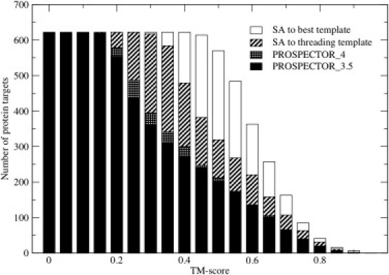
Cumulative number of protein targets whose TM-score is less than or equal to the TM-score threshold specified on the abscissa (solid representation) for the best of top five PROSPECTOR_3.5 threading alignments; (cross-hatched), the best of top five PROSPECTOR_4 threading alignments; (diagonal pattern), the best structural alignment of the top five ranked PROSPECTOR_4 templates; and (open representation), the best structural alignment, SA, to any protein in the structural template library.
Let the number of fragments predicted for target residue i be nf. For each of these fragments, using the Kabsch rotation matrix that minimizes the root mean-square deviation (RMSD) between the fragment and the template (36), we calculate a pseudo TM-score between the kth such fragment as
| (6a) |
Let dij be the distance between fragment residue i and template residue j after optimal superposition. If dij > d0, then
| (6b) |
Otherwise,
| (6c) |
We have set d0 = 2 Å. The goal of Eq. 6 is to strongly penalize fragments whose geometry disagrees with that of the template. In practice, we take the fragment that gives maximum value over all the fragments,
We then calculate the score matrix between target residue i and template residue j as
| (7a) |
when
and
| (7b) |
Based on training set optimization, af = 0.1, and we take the gap opening and propagation parameters as in PROSPECTOR_4.
After generating the fragment library template alignment, if the z-score of the template from PROSPECTOR_4 >20, each predicted target contact extracted from the target-template alignment is assigned a weight of 2; otherwise, it is assigned a weight of 1. For those contacts whose weight is >1, we add an additional weight of 1 if the BLOSUM62 mutation matrix associated with contacting pairs within ±3 residues of an aligned target-template pair is positive. Finally, we examine the contact weight matrix and assign a residue pair as being in contact if their contact weight matrix >1 and the residues are at least five amino-acids apart in the protein sequence. In practice, two fragment libraries (generated when difference fragment similarity cutoffs are used), so that the STITCH algorithm provides two sets of predicted contacts for each target protein.
In a similar fashion, we can generate tentative target-template alignments. The simplest approach would be to just take the aligned template residues. However, we have found better results if we use the template as a reference frame to generate the local alignment of the up to ℓ fragments that have a template residue i′ associated with template fragment j′. In practice, we generate the superposition of all (up to ℓ) aligned fragments that contain residue i. The average value of the coordinates associated with the ith residue is taken to be its predicted coordinates. Once again, because two fragment libraries are used, each provides a set of five structural predictions.
Confidence-weighted contact predictions in TASSER_WT
Each of the four threading algorithms, PROSPECTOR_3, PROSPECTOR_4, STITCH_low, and STITCH_high, provide a set of predicted contacts. The weight of a predicted contact, wt(i,j), is the sum of the number of times the contact appears in the four methods; we term this method of side-chain contact prediction, COMBCON. In practice, wt(i,j) ranges from 1 to 4. As shown below, the contacts become more accurate as their weight increases. To increase the effect of these contact restraints in TASSER, we introduce a modified contact restraint function into TASSER_WT. When the ith and jth residues are in contact as predicted by COMBCON, their contact energy (Eadd–wt) is defined by
| (8) |
where r(i,j) is the distance between the side-chain centers of mass of the ith and jth residues, r0(i,j) is the corresponding cutoff distance for a contact between their side-chain centers of mass, and wt(i,j) is the corresponding confidence weight.
Structure assembly and final model selection
Besides the additional contact-weighted restraints of Eq. 8, the energy function of TASSER_WT is identical to that of TASSER_2.0 (14) and is composed of knowledge-based long- and short-range correlations, the propensity for predicted secondary structures, protein specific pair interactions, and a residue-based solvent accessibility term. The protein representation (Cα atoms and the side-chain centers of mass) and conformational search scheme, Parallel Hyperbolic Monte Carlo Sampling (37), are the same as in the original TASSER (13). The resulting structures are clustered using SPICKER (38), and the top five models from the 14 lowest temperature replicas constitute the set of predicted structures.
Benchmark proteins and template library
For benchmarking TASSER_WT, we use 622 Hard targets from the previous benchmark test set of 2591 nonhomologous single domain proteins having ≤ 200 residues (14). (The list is provided at http://cssb.biology.gatech.edu/skolnick/files/TASSER_WT/LIST.Hard.) These benchmark proteins have <35% sequence identity to each other. (The structure template library used by all four approaches is available at http://cssb.biology.gatech.edu/skolnick/files/TASSER_WT/LIST.templates.) All targets have <30% sequence identity to their closest template, with an average pairwise sequence identity of 13.3%.
Results and Discussion
Comparison of PROSPECTOR_3.5, PROSPECTOR_4, and the best structural alignments
In Fig. 2, for the 622-protein benchmark set, we present a histogram of the cumulative number of proteins whose best of top five templates has a TM-score greater than or equal to the specified value for PROSPECTOR_3.5 (solid), PROSPECTOR_4 (cross-hatched), the structural alignment, SA, of the best of top five PROSPECTOR_4 templates to the native structure obtained using fr-TM align (29) (diagonal stripes), and the best SA of the target to the entire template library (open histogram). Comparing PROSPECTOR_3.5 with PROSPECTOR_4, the average TM-score increases from 0.409 to 0.424, but, most importantly, the number of targets whose TM-score ≥0.4 increases from 270 to 292, an 8% improvement.
Indeed, it is over the TM-score range of 0.4–0.5 where there is significant improvement in the template alignment quality. We note, however, that the best structural alignment of the top five PROSPECTOR_4 templates to their corresponding native structure gives significantly better results over the entire TM-score range, with a mean TM-score of 0.535, and 479 (77%) of the targets having a TM-score ≥0.4. This validates our previous statement that the PROSPECTOR_4 selected templates could, in principle, be used to generate better results even when their actual alignment quality is quite poor. The average pairwise target-template sequence identity of the best of top five templates is 13.5% from PROSPECTOR_4 as compared to 9.4% from their corresponding best structural alignment to native. Finally, consistent with the likely completeness of the PDB (39), all targets have a good structural alignment to some member of the PDB library with an average best TM-score of 0.634 and sequence identity of 9.9%. Thus, considerable improvement could result if we had a means of selecting the best templates and their associated structural alignments.
Can we exploit the above insights to generate better alignments?
On applying STITCH_high to the top 30 templates identified by PROSPECTOR_4, we found that the average TM-score is 0.35, with an average coverage (fraction of aligned residues) of 0.62. Similarly, STITCH_low generated alignments, with the best of top five TM-scores of 0.37 and 0.71 average coverage. At first glance, this might appear to be discouraging as compared to PROSPECTOR_4. However, as shown in Fig. 3, A and B, there are significantly more low RMSD alignments at acceptable coverage (fraction of target residues aligned to the template) as compared to PROSPECTOR_4 or PROSPECTOR_3.5 (which has somewhat poorer performance than PROSPECTOR_4). The more accurate alignments as selected by STITCH_high as compared to STITCH_low are at the expense of lower coverage. We note that STITCH_high (STITCH_low) has 350 (292) targets with a RMSD ≤6 Å. This suggests that the template alignments generated by STITCH could be profitably used to select more accurate predicted tertiary contact restraints, a point we now demonstrate.
Figure 3.
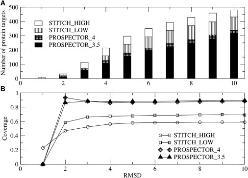
(A) Cumulative fraction of the number of protein targets whose best of top five templates has an RMSD less than or equal to the root mean-squared deviation (RMSD) value specified on the abscissa. (B) Corresponding cumulative average coverage for templates with an RMSD to native less than or equal to the RMSD specified on the abscissa (open representation) from STITCH_high, the higher confidence fragment library (striped representation) from STITCH_low, the lower confidence fragment library, from PROSPECTOR_4 (cross-hatched), and from PROSPECTOR_3.5 (solid representation).
Contact restraint prediction
To assess the quality of the predicted contact restraints, we calculate the fraction of accurately predicted contacts (Facc) and the fraction of predicted contacts per residue by
| (9a) |
| (9b) |
where Nc,c is the number of common contacts in both the predicted contact restraints and the native structure, Nc,a is the total number of the predicted contacts, and Nres is the length of the target protein. Contact restraints from COMBCON have a confidence weight ranging from 1 to 4. The higher weight indicates more confidently predicted contact restraints. In what follows, Fwt≥macc and Fwt≥mcov indicate Facc and Fcov at a confidence weight ≥m, respectively.
As shown in Table 2, for contact restraints with weight ≥1 and ≥2, the average Fwt≥1acc and Fwt≥2acc with ±SD (standard deviation) is 0.21 ± 0.15 and 0.40 ± 0.25, respectively. The accuracy of these predicted contact restraints (especially Fwt≥1acc) is too low to expect a reasonably accurate TASSER model. However, the average Fwt≥3acc and Fwt≥4acc from COMBCON is 0.57 ± 0.32 and 0.67 ± 0.32, respectively. Predicted contact restraints with confidence weights = 4 have improved accuracy, compared with 0.60 ± 0.33 of TASSER_2.0.
Table 2.
Fraction of accurately predicted contacts and predicted number of contacts per residue with confidence weight ≥3 from COMBCON and TASSER_2.0
| COMBCON |
TASSER_2.0 |
||||
|---|---|---|---|---|---|
| Weight∗ | No.† | Fwtacc‡ [SD] | Fwtcov§(Contacts/residue) [SD] | Facc¶ [SD] | Fcov‖(Contacts/residue) [SD] |
| ≥4 | 346 | 0.67 [0.32] | 0.48 [0.63] | 0.60 [0.30] | 0.36 [0.44] |
| ≥3 | 454 | 0.57 [0.32] | 0.51 [0.65] | 0.56 [0.32] | 0.29 [0.40] |
| ≥2 | 620 | 0.40 [0.25] | 0.87 [0.91] | 0.50 [0.34] | 0.25 [0.37] |
| ≥1 | 622 | 0.21 [0.15] | 3.65 [1.15] | 0.50 [0.34] | 0.25 [0.37] |
SD = standard deviation.
Confidence weight from COMBCON.
Number of targets in each category from COMBCON.
Average fraction of accurately predicted contact restraints from COMBCON.
Average fraction of predicted contacts per residue from COMBCON.
Average fraction of accurately predicted contact restraints from TASSER_2.0 for the same targets of each category.
Average fraction of predicted contacts per residue from TASSER_2.0 for the same targets of each category.
More importantly, TASSER_WT's coverage is considerably higher, with values of 0.51 ± 0.65 and 0.48 ± 0.63 Fwtcov = 3 and 4 as compared to 0.29 ± 0.4 and 0.36 ± 0.44 of TASSER_2.0 for the identical proteins. In COMBCON, unlike TASSER_2.0, according to their confidence weights, the more accurately contact restraints can be identified among all predicted contacts. Among 622 Hard targets, 454 have at least one predicted contact with confidence weight ≥3. Thus, because it is the number of accurately predicted contacts/residue at high confidence which dictates the performance of TASSER, we would expect better results from TASSER_WT as compared to TASSER_2.0.
Based on their accuracy/coverage, for TASSER_WT, we will use the predicted contact restraints with confidence weight ≥3 from COMBCON using Eq. 8, while contacts with the confidence weight = 2 are very weakly incorporated into TASSER_WT. We do not use contact restraints with the confidence weight = 1 in TASSER_WT because their accuracy is extremely low.
TASSER_WT refinement results
In what follows, we focus on the TASSER_WT prediction for the 454/622 Hard targets that have at least one predicted contact with confidence weight ≥3, because for the remaining 168 targets, COMBCON provides very low accuracy contact predictions.
In Table 3, we show the average RMSD and TM-score to the native structure of the top and best-of-top-five ranked TASSER_2.0 and TASSER_WT models with Fwt≥3cov of COMBCON. When Fwt≥3cov > 0.0, the average RMSD (±SD) of the best-of-top-five (top-ranked) ranked TASSER_WT models is 7.44 ± 4.23 Å (8.74 ± 4.84 Å), whereas TASSER_2.0 models have an average RMSD of 7.79 ± 4.09 Å (9.45 ± 4.79Å). When Fwt≥3cov > 0.4, TASSER_WT (TASSER_2.0) best-of-top-five models have an average RMSD of 5.03 ± 3.09 Å (6.40 ± 3.65 Å). When Fwt≥3cov >1.0, TASSER_WT (TASSER_2.0) best-of-top-five models have an average RMSD of 4.11 ± 2.38 Å (6.72 ± 3.80 Å).
Table 3.
Comparison of models from TASSER_WT and TASSER_2.0
| 〈RMSD to the native〉 (SD∗), Å |
〈TM-score to the native〉 (SD) |
||||||||
|---|---|---|---|---|---|---|---|---|---|
| Top1 |
Best |
Top1 |
Best |
||||||
| Fwt≥3cov | No.∗ | M2.0† | MWT‡ | M2.0§ | MWT¶ | M2.0TM‖ | MWTTM∗∗ | M2.0TM†† | MWTTM‡‡ |
| >1.0 | 80 | 8.48 (4.62) | 4.71 (3.03) | 6.72 (3.80) | 4.11 (2.38) | 0.525 (0.192) | 0.738 (0.104) | 0.570 (0.184) | 0.743 (0.104) |
| >0.8 | 104 | 8.30 (4.60) | 5.26 (3.33) | 6.54 (3.74) | 4.40 (2.53) | 0.535 (0.186) | 0.714 (0.116) | 0.580 (0.176) | 0.719 (0.113) |
| >0.6 | 130 | 8.05 (4.51) | 5.56 (3.72) | 6.38 (3.65) | 4.70 (3.00) | 0.531 (0.190) | 0.685 (0.151) | 0.574 (0.177) | 0.692 (0.147) |
| >0.4 | 175 | 8.11 (4.70) | 6.02 (3.83) | 6.40 (3.65) | 5.03 (3.09) | 0.530 (0.181) | 0.655 (0.160) | 0.570 (0.169) | 0.667 (0.156) |
| >0.2 | 224 | 7.95 (4.55) | 6.37 (3.96) | 6.37 (3.54) | 5.40 (3.28) | 0.529 (0.176) | 0.631 (0.166) | 0.567 (0.165) | 0.644 (0.164) |
| >0.0 | 454 | 9.45 (4.79) | 8.74 (4.84) | 7.79 (4.09) | 7.44 (4.23) | 0.455 (0.180) | 0.506 (0.199) | 0.489 (0.175) | 0.526 (0.195) |
SD∗ is the average standard deviation of the models, shown in parentheses.
Number of targets in each category.
Top1: Average RMSD to the native structure of top model among the top five. TASSER_2.0 model.
Top1: Average RMSD to the native structure of top model among the top five. TASSER_WT model.
Best: Average RMSD to the native structure of the best model among the top five. TASSER_2.0 model.
Best: Average RMSD to the native structure of the best model among the top five. TASSER_WT model.
Top1: Average TM-score to the native structure of top1 model among the top five. TASSER_2.0 model.
Top1: Average TM-score to the native structure of top1 model among the top five. TASSER_WT model.
Best: Average TM-score to the native structure of the best model among the top five. TASSER_2.0 model.
Best: Average TM-score to the native structure of the best model among the top five. TASSER_WT model.
In Table 3, we also present the TM-score of the predicted models to the native structure (40). For targets having Fwt≥3cov > 1.0, the average TM-score of the best-of-top-five TASSER_WT (TASSER_2.0) models is 0.743 ± 0.104 (0.570 ± 0.184). Even when Fwt≥3cov > 0.0, the best-of-top-five (top) TASSER_WT models have an average TM-score of 0.526 ± 0.195 (0.506 ± 0.199), compared to 0.489 ± 0.175 (0.455 ± 0.180) for TASSER_2.0 models.
These results show that:
-
1.
When COMBCON provides at least one contact restraint with confidence weight ≥3, TASSER_WT outperforms TASSER_2.0.
-
2.
As the number of contacts with confidence weight ≥3 (Fwt≥3cov) is increased, TASSER_WT models become much closer to their native structure than TASSER_2.0 models.
Fig. 4 shows the cumulative fraction of targets with an RMSD difference between the best-of-top-five TASSER_WT and TASSER_2.0 models, ΔRMSD (RMSDTASSER_WT – RMSDTASSER_2.0) less than the specified ΔRMSD value when Fwt≥3cov > 0.0, 0.4, and 1.0. When the ΔRMSD is negative, the TASSER_WT model has a smaller RMSD to the native structure than the TASSER_2.0 model. When Fwt≥3cov > 1.0, 79% of the TASSER_WT models become closer to the native than the TASSER_2.0 models. When Fwt≥3cov > 0.4 and > 0.0, 66% and 52% of the TASSER_WT models, respectively, have a smaller RMSD to native value than the TASSER_2.0 models. For those models that are closer to native than the corresponding TASSER_2.0 models, when Fwt≥3cov > 1.0, 81% and 73% of the TASSER_WT models have an RMSD improvement >0.5 Å and 1.0 Å, respectively. As the Fwt≥3cov increases, TASSER_WT significantly outperforms TASSER_2.0 because the accuracy of the predicted contacts produces better quality structures.
Figure 4.
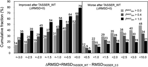
Cumulative fraction of the RMSD difference between the TASSER_WT and TASSER_2.0 models with the fraction of predicted contacts per residue of the confidence weight ≥3 (Fwt≥3cov) where RMSDTASSER_WT and RMSDTASSER_2.0 is the RMSD of TASSER_WT and TASSER_2.0 models to the native structure, respectively. The RMSD is negative when the TASSER_WT model has a smaller RMSD than the TASSER_2.0 model.
Fig. 5, a–f, presents representative examples showing the improvement of the TASSER_WT models over the TASSER_2.0 models. For 3inkC (Fig. 5, a and b, an α-helical protein), the TASSER_2.0 model was predicted with contacts having a Facc of 1.00 and Fcov of 0.02; the resulting model has an RMSD to the native structure of 7.9 Å. The TASSER_WT model has a RMSD of 4.0 Å for which Fwt≥3acc (Fwt≥3cov) is 0.69 (1.22). For 1bcpD (Fig. 5, c and d, a β-protein), the RMSD of the TASSER_WT model predicted, with a Fwt≥3acc (Fwt≥3cov) of 0.61 (2.69), is 4.2 Å. This is much smaller than the RMSD of 11.0 Å of the TASSER_2.0 model generated with Facc of 0.00 and Fcov 0.04. For 1ogcA (Fig. 5, e and f, an α/β protein), the TASSER_WT (TASSER_2.0) model has an RMSD of 3.2 Å (10.5 Å), where Fwt≥3acc (Facc) and Fwt≥3cov (Fcov) are 0.66 (0.67) and 3.50 (0.09), respectively. These examples clearly demonstrate that increased contact prediction accuracy is responsible for the improvement of TASSER_WT over TASSER_2.0 models.
Figure 5.
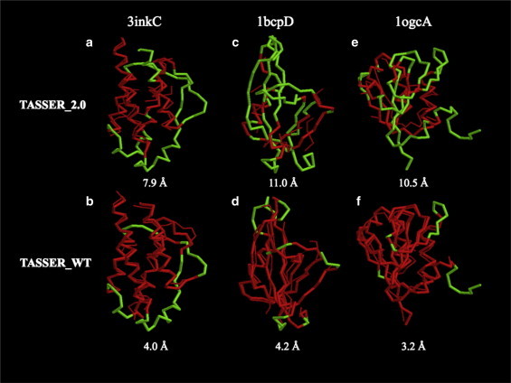
Representative examples showing the improvement of TASSER_WT models over TASSER_2.0 models for 3inkC (α-protein), 1bcpD (β-protein), and 1ogcA (α/β protein) in the Hard set. The thick (thin) line refers to the native structure (predicted model). Red indicates residue pairs having a distance <5 Å after superposition of the predicted model onto the native structure. For the remainder of residues whose distance is ≥5 Å after superposition, the native structure is shown in green. Below the models is the RMSD to the native structure.
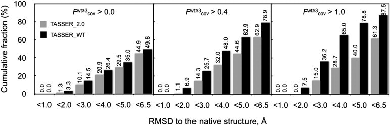
In Fig. 6, we show the cumulative histogram of the RMSD of the TASSER_2.0 and TASSER_WT models for different Fwt≥3acc thresholds. We can define a foldable protein when the RMSD of a predicted model to the native structure is <6.5 Å (13,14,20). For Fwt≥3cov > 1.0, the fraction of foldable proteins of TASSER_WT (TASSER_2.0) models is 87.5% (61.3%). When Fwt≥3cov > 0.4 TASSER_WT (TASSER_2.0) models have a success rate of 78.9% (62.9%). When Fwt≥3cov > 0.0, the success rate of the TASSER_WT (TASSER_2.0) models drops to 49.6% (44.9%).
Figure 6.
Cumulative fraction of the cumulative RMSD distribution of WT-TASSER and TASSER_2.0 models having a fraction of predicted contacts per residue whose confidence weight is ≥3 at different values of the coverage Fwt≥3cov.
Alternatively, if we define the fraction of foldable proteins as those with TM-scores ≥0.4, then for Fwt≥3cov > 1.0, the fraction of foldable proteins of the TASSER_WT (TASSER_2.0) models is 98.8% (76.2%). When Fwt≥3cov > 0.4, the TASSER_WT (TASSER_2.0) models have a success rate of 93.7% (81.1%). When Fwt≥3cov > 0.0, the success rate of the TASSER_WT (TASSER_2.5) models drops to 69.6% (64.3%). Thus, by both metrics, TASSER_WT has a larger number of foldable target proteins.
We next examine the fraction of target proteins not foldable by TASSER_2.0 but which are foldable using TASSER_WT. TASSER_WT converts 28.7, 20.6, and 11.9% of these targets into foldable proteins when Fwt≥3cov > 1.0, > 0.4, and > 0.0, respectively. Overall, TASSER_WT improves the fraction of foldable proteins; in particular, the largest improvement is seen when Fwt≥3cov > 1.0, because the predicted contact restraints have both high accuracy and a large number of such accurately predicted contacts per residue.
Conclusions
To improve the prediction accuracy of TASSER for the most difficult Hard targets, we have developed TASSER_WT, which uses the more accurate contact restraints from COMBCON. COMBCON provides contact restraints with a confidence weight that successfully distinguishes the more accurately predicted contacts among all predicted contact restraints; this a priori knowledge is very useful for TASSER structure prediction.
Here, we examined the performance of TASSER_WT on the 622 Hard targets of the previous benchmark set consisting of 2591 nonhomologous, single domain protein targets (14). Previously, the prediction accuracy for these targets was poor because the average quality of the template alignments was quite bad. By using consensus-weighted contacts extracted from variants of PROSPECTOR as well as a new fragment-based threading method, STITCH, TASSER_WT shows significant improvement over TASSER_2.0 for those targets having higher confidence restraints. By incorporating contact restraints with both high accuracy and high contact coverage, TASSER_WT significantly increases the prediction accuracy for the majority of the Hard targets. This work suggests that for the regime of the most difficult targets, template-based approaches for protein structure prediction can make significant progress for the remaining 20% or so of single domain proteins for which template identification has not yet been successful.
The key new insight of this approach is the fact that even for Hard targets, existing threading algorithms can often identify templates whose structural alignments to the native structure are quite good, even though the actual threading alignment quality is quite poor. The outstanding problem is to better identify these good alignments.
The STITCH fragment-based, threading approach is designed to take a step in this direction. By selecting the better predicted regions in the template alignments, this enables one to extract, more accurately, predicted side-chain contacts at acceptable levels of coverage. These then allow for better models to be generated by TASSER_WT. Additional work that further incorporates information provided by structural fragments with the goal of generating even better quality alignments is currently underway.
Acknowledgments
Stimulating discussions with Dr. Michal Brylinski are gratefully acknowledged.
This research was supported by grants Nos. GM-48835 and GM-37408 of the Division of General Medical Sciences of the National Institutes of Health, Bethesda, MD.
References
- 1.Murzin A.G. Progress in protein structure prediction. Nat. Struct. Biol. 2001;8:110–112. doi: 10.1038/84088. [DOI] [PubMed] [Google Scholar]
- 2.Pillardy J., Czaplewski C., Scheraga H.A. Recent improvements in prediction of protein structure by global optimization of a potential energy function. Proc. Natl. Acad. Sci. USA. 2001;98:2329–2333. doi: 10.1073/pnas.041609598. [DOI] [PMC free article] [PubMed] [Google Scholar]
- 3.Skolnick J. In quest of an empirical potential for protein structure prediction. Curr. Opin. Struct. Biol. 2006;16:166–171. doi: 10.1016/j.sbi.2006.02.004. [DOI] [PubMed] [Google Scholar]
- 4.DeBartolo J., Colubri A., Sosnick T.R. Mimicking the folding pathway to improve homology-free protein structure prediction. Proc. Natl. Acad. Sci. USA. 2009;106:3734–3739. doi: 10.1073/pnas.0811363106. [DOI] [PMC free article] [PubMed] [Google Scholar]
- 5.Kryshtafovych A., Krysko O., Fidelis K. Protein structure prediction center in CASP8. Proteins. 2009;77(Suppl 9):5–9. doi: 10.1002/prot.22517. [DOI] [PMC free article] [PubMed] [Google Scholar]
- 6.Zhao F., Peng J., Xu J. A probabilistic and continuous model of protein conformational space for template-free modeling. J. Comput. Biol. 2010;17:783–798. doi: 10.1089/cmb.2009.0235. [DOI] [PMC free article] [PubMed] [Google Scholar]
- 7.Hardin C., Pogorelov T.V., Luthey-Schulten Z. Ab initio protein structure prediction. Curr. Opin. Struct. Biol. 2002;12:176–181. doi: 10.1016/s0959-440x(02)00306-8. [DOI] [PubMed] [Google Scholar]
- 8.Gopal S.M., Klenin K., Wenzel W. Template-free protein structure prediction and quality assessment with an all-atom free-energy model. Proteins. 2009;77:330–341. doi: 10.1002/prot.22438. [DOI] [PubMed] [Google Scholar]
- 9.Ben-David M., Noivirt-Brik O., Levy Y. Assessment of CASP8 structure predictions for template free targets. Proteins. 2009;77(Suppl 9):50–65. doi: 10.1002/prot.22591. [DOI] [PubMed] [Google Scholar]
- 10.Marchler-Bauer A., Bryant S.H. A measure of progress in fold recognition? Proteins. 1999;3(Suppl):218–225. doi: 10.1002/(sici)1097-0134(1999)37:3+<218::aid-prot28>3.3.co;2-o. [DOI] [PubMed] [Google Scholar]
- 11.Panchenko A.R., Marchler-Bauer A., Bryant S.H. Combination of threading potentials and sequence profiles improves fold recognition. J. Mol. Biol. 2000;296:1319–1331. doi: 10.1006/jmbi.2000.3541. [DOI] [PubMed] [Google Scholar]
- 12.Zhang Y. I-TASSER: fully automated protein structure prediction in CASP8. Proteins. 2009;77(Suppl 9):100–113. doi: 10.1002/prot.22588. [DOI] [PMC free article] [PubMed] [Google Scholar]
- 13.Zhang Y., Skolnick J. Automated structure prediction of weakly homologous proteins on a genomic scale. Proc. Natl. Acad. Sci. USA. 2004;101:7594–7599. doi: 10.1073/pnas.0305695101. [DOI] [PMC free article] [PubMed] [Google Scholar]
- 14.Lee S.Y., Skolnick J. Benchmarking of TASSER_2.0: an improved protein structure prediction algorithm with more accurate predicted contact restraints. Biophys. J. 2008;95:1956–1964. doi: 10.1529/biophysj.108.129759. [DOI] [PMC free article] [PubMed] [Google Scholar]
- 15.Simons K.T., Strauss C., Baker D. Prospects for ab initio protein structural genomics. J. Mol. Biol. 2001;306:1191–1199. doi: 10.1006/jmbi.2000.4459. [DOI] [PubMed] [Google Scholar]
- 16.Shan Y., Wang G., Zhou H.X. Fold recognition and accurate query-template alignment by a combination of PSI-BLAST and threading. Proteins. 2001;42:23–37. doi: 10.1002/1097-0134(20010101)42:1<23::aid-prot40>3.0.co;2-k. [DOI] [PubMed] [Google Scholar]
- 17.Daga P.R., Patel R.Y., Doerksen R.J. Template-based protein modeling: recent methodological advances. Curr. Top. Med. Chem. 2010;10:84–94. doi: 10.2174/156802610790232314. [DOI] [PMC free article] [PubMed] [Google Scholar]
- 18.Bernstein F.C., Koetzle T.F., Tasumi M. The Protein DataBank: a computer-based archival file for macromolecular structures. J. Mol. Biol. 1977;112:535–542. doi: 10.1016/s0022-2836(77)80200-3. [DOI] [PubMed] [Google Scholar]
- 19.Zhang Y., Arakaki A.K., Skolnick J. TASSER: an automated method for the prediction of protein tertiary structures in CASP6. Proteins. 2005;61(Suppl 7):91–98. doi: 10.1002/prot.20724. [DOI] [PubMed] [Google Scholar]
- 20.Zhang Y., Skolnick J. Tertiary structure predictions on a comprehensive benchmark of medium to large size proteins. Biophys. J. 2004;87:2647–2655. doi: 10.1529/biophysj.104.045385. [DOI] [PMC free article] [PubMed] [Google Scholar]
- 21.Lee S.Y., Skolnick J. Development and benchmarking of TASSER(iter) for the iterative improvement of protein structure predictions. Proteins. 2007;68:39–47. doi: 10.1002/prot.21440. [DOI] [PubMed] [Google Scholar]
- 22.Zhou H., Pandit S.B., Skolnick J. Analysis of TASSER-based CASP7 protein structure prediction results. Proteins. 2007;69(Suppl 8):90–97. doi: 10.1002/prot.21649. [DOI] [PubMed] [Google Scholar]
- 23.Zhou H., Skolnick J. Ab initio protein structure prediction using chunk-TASSER. Biophys. J. 2007;93:1510–1518. doi: 10.1529/biophysj.107.109959. [DOI] [PMC free article] [PubMed] [Google Scholar]
- 24.Zhou H., Skolnick J. Protein structure prediction by pro-Sp3-TASSER. Biophys. J. 2009;96:2119–2127. doi: 10.1016/j.bpj.2008.12.3898. [DOI] [PMC free article] [PubMed] [Google Scholar]
- 25.Lee S.Y., Zhang Y., Skolnick J. TASSER-based refinement of NMR structures. Proteins. 2006;63:451–456. doi: 10.1002/prot.20902. [DOI] [PubMed] [Google Scholar]
- 26.Borreguero J.M., Skolnick J. Benchmarking of TASSER in the ab initio limit. Proteins. 2007;68:48–56. doi: 10.1002/prot.21392. [DOI] [PubMed] [Google Scholar]
- 27.Skolnick J., Kihara D. Defrosting the frozen approximation: PROSPECTOR—a new approach to threading. Proteins. 2001;42:319–331. [PubMed] [Google Scholar]
- 28.Skolnick J., Kihara D., Zhang Y. Development and large scale benchmark testing of the PROSPECTOR_3 threading algorithm. Proteins. 2004;56:502–518. doi: 10.1002/prot.20106. [DOI] [PubMed] [Google Scholar]
- 29.Pandit S.B., Skolnick J. Fr-TM-align: a new protein structural alignment method based on fragment alignments and the TM-score. BMC Bioinformatics. 2008;9:531. doi: 10.1186/1471-2105-9-531. [DOI] [PMC free article] [PubMed] [Google Scholar]
- 30.Zhang Y., Skolnick J. The protein structure prediction problem could be solved using the current PDB library. Proc. Natl. Acad. Sci. USA. 2005;102:1029–1034. doi: 10.1073/pnas.0407152101. [DOI] [PMC free article] [PubMed] [Google Scholar]
- 31.Henikoff S., Henikoff J.G. Performance evaluation of amino acid substitution matrices. Proteins. 1993;17:49–61. doi: 10.1002/prot.340170108. [DOI] [PubMed] [Google Scholar]
- 32.Altschul S.F., Koonin E.V. Iterated profile searches with PSI-BLAST—a tool for discovery in protein databases. Trends Biochem. Sci. 1998;23:444–447. doi: 10.1016/s0968-0004(98)01298-5. [DOI] [PubMed] [Google Scholar]
- 33.Skolnick J., Kolinski A., Ortiz A. Derivation of protein-specific pair potentials based on weak sequence fragment similarity. Proteins. 2000;38:3–16. [PubMed] [Google Scholar]
- 34.Tanaka S., Scheraga H.A. Medium- and long-range interaction parameters between amino acids for predicting three-dimensional structures of proteins. Macromolecules. 1976;9:945–950. doi: 10.1021/ma60054a013. [DOI] [PubMed] [Google Scholar]
- 35.Zhang Y., Skolnick J. TM-align: a protein structure alignment algorithm based on the TM-score. Nucleic Acids Res. 2005;33:2302–2309. doi: 10.1093/nar/gki524. [DOI] [PMC free article] [PubMed] [Google Scholar]
- 36.Kabsch W. Solution for the best rotation to relate two sets of vectors. Acta Crystallogr. A. 1976;32:922–923. [Google Scholar]
- 37.Zhang Y., Kihara D., Skolnick J. Local energy landscape flattening: parallel hyperbolic Monte Carlo sampling of protein folding. Proteins. 2002;48:192–201. doi: 10.1002/prot.10141. [DOI] [PubMed] [Google Scholar]
- 38.Zhang Y., Skolnick J. SPICKER: a clustering approach to identify near-native protein folds. J. Comput. Chem. 2004;25:865–871. doi: 10.1002/jcc.20011. [DOI] [PubMed] [Google Scholar]
- 39.Zhang Y., Hubner I.A., Skolnick J. On the origin and highly likely completeness of single-domain protein structures. Proc. Natl. Acad. Sci. USA. 2006;103:2605–2610. doi: 10.1073/pnas.0509379103. [DOI] [PMC free article] [PubMed] [Google Scholar]
- 40.Zhang Y., Skolnick J. Scoring function for automated assessment of protein structure template quality. Proteins. 2004;57:702–710. doi: 10.1002/prot.20264. [DOI] [PubMed] [Google Scholar]