Characterization of Brightness and Stoichiometry of Bright Particles by Flow-Fluorescence Fluctuation Spectroscopy

Abstract

Characterization of bright particles at low concentrations by fluorescence fluctuation spectroscopy (FFS) is challenging, because the event rate of particle detection is low and fluorescence background contributes significantly to the measured signal. It is straightforward to increase the event rate by flow, but the high background continues to be problematic for fluorescence correlation spectroscopy. Here, we characterize the use of photon-counting histogram analysis in the presence of flow. We demonstrate that a photon-counting histogram efficiently separates the particle signal from the background and faithfully determines the brightness and concentration of particles independent of flow speed, as long as undersampling is avoided. Brightness provides a measure of the number of fluorescently labeled proteins within a complex and has been used to determine stoichiometry of protein complexes in vivo and in vitro. We apply flow-FFS to determine the stoichiometry of the group specific antigen protein within viral-like particles of the human immunodeficiency virus type-1 from the brightness. Our results demonstrate that flow-FFS is a sensitive method for the characterization of complex macromolecular particles at low concentrations.

Introduction

Fluorescence fluctuation spectroscopy (FFS) uses the signal fluctuations generated by individual fluorescent particles passing through a small optical observation volume to characterize the sample (1,2). Analysis of the intensity correlation function, which is known as fluorescence correlation spectroscopy (FCS), determines the concentration and temporal properties of the particles (3). Photon-counting histogram (PCH) and related techniques (4–6) extract from the data the brightness and the average particle occupation number within the observation volume. Brightness, which is defined as the average fluorescence intensity of a single fluorescent particle or molecule, encodes the stoichiometry of a protein complex. This concept was experimentally verified using green fluorescent protein (GFP) as a marker and has been applied to study the concentration-dependent oligomerization of proteins in living cells (7). The same concept has been extended to dual-color brightness studies of hetero-protein complexes in cells (8,9). Although most studies have focused on cellular applications, brightness analysis is also valuable for the characterization of protein complexes in vitro (10). In fact, a recent study demonstrated that FFS is a suitable in vitro technique for the characterization of viral-like particles (VLPs) that contain hundreds to thousands of copies of labeled proteins (11). However, studying these large protein complexes presents a unique set of challenges that this article will address.

Biological particles, such as viruses and vesicles, are relatively large and contain tens to thousands of proteins. These particles can be hard to study using FCS, because they often exist at very low concentrations and diffuse slowly due to their large size. Thus, particles are infrequently detected, which necessitates very long data acquisition times to build up the required statistics for FFS analysis. Often such experiments cannot be performed, because the measurement time is exorbitant. Flowing or moving the sample during data acquisition is a simple method to significantly increase the event rate of particles passing through the observation volume (12). This article focuses on FFS measurements of flowing samples, which we refer to as flow-FFS. We further refer to FFS measurements on a resting sample as stationary-FFS to contrast the two methods. Although the effect of flow on the autocorrelation function is well known (13), the influence of flow on PCH and brightness has not yet been investigated. Here, we characterize flow-FFS and demonstrate that brightness and concentration determined by PCH analysis are unaffected by flow speed as long as undersampling is avoided. We further provide guidance on optimizing flow-FFS through the proper selection of flow speed and sampling time.

Even in the presence of flow, FCS experiments at low concentrations remain challenging. The fluorescence background of samples at subnanomolar concentrations often overwhelms the contributions from the particles and consequently reduces the fluctuation amplitude of the autocorrelation function. Differentiating between the particle signal and the background based on the autocorrelation function of a flowing sample is not feasible. Remarkably, PCH, unlike autocorrelation analysis, has the capability of separating the signal of sparse but bright particles from the background. This property of PCH is crucial for quantitative characterization of the brightness and concentration of particles at very low concentrations. We characterize flow-FFS on fluorescent microspheres flowing through a microfluidic channel in concentrations ranging from 1 nM to 10 fM. Next, flow-FFS and stationary-FFS are applied to determine the stoichiometry of the human immunodeficiency virus type-1 (HIV-1) Gag (group-specific antigen) polyprotein within VLPs. We demonstrate that flow-FFS determines the stoichiometry from VLPs at lower concentrations and at significantly shorter data acquisition times than for stationary-FFS. This study establishes the utility of flow-FFS as a sensitive tool to gain quantitative information regarding the composition of complex macromolecular particles.

Material and Methods

Experimental setup

The experiments were carried out on a modified two-photon microscope, as previously described (7), using two-photon excitation at a wavelength of 905 nm. The fluorescent microspheres and VLPs were measured with a Zeiss 63× C-Apochromat water immersion objective (NA 1.2) with excitation powers ranging from 0.1 to 1.0 mW as measured after the objective. FFS data are acquired at sampling frequencies from 20 to 200 kHz, stored, and subsequently analyzed with programs written for IDL version 6.4 (RSI, Boulder, CO).

Stationary measurements were performed by loading 200 μL of solution into an eight-well Nunc Lab-Tek Chamber Slide (Thermo Fisher Scientific, Pittsburgh PA). Flow measurements were performed at the center of a 20-μm-tall microfluidic channels with widths ranging from 20 to 200 μm. Constant pressure-driven flow was achieved using a syringe pump (Kent Scientific, Torrington, CT). Flow velocities ranging from 2 to 44 mm/s were measured at the center of the channel. Fabrication of the microchannel devices and sample preparation of the microspheres and fluorescently labeled VLPs are described in the Supporting Material.

Data analysis

The autocorrelation function of stationary-FFS measurements was fit to a single species diffusion model,

$$g_{\text{D}}\left(\tau \right)=g\left(0\right){\left(1+\raisebox{1ex}{$\tau $}\!\left/ \!\raisebox{-1ex}{${\tau }_{\text{D}}$}\right.\right)}^{-1}.$$ (1)

This equation provided a sufficient approximation to determine the fluctuation amplitude, $g\left(0\right)$, and the diffusion time, ${\tau }_{\text{D}}=w_0^2/(4nD)$. This relation allows us to calculate the diffusion coefficient, D, once the radial beam waist, $w_0$, is known. Because the experiments are conducted with two-photon excitation, we set n = 2. In the presence of uniform flow with velocity $v_{\text{F}}$ the autocorrelation function decays more quickly. FFS measurements of flowing samples were conducted at flow speeds where diffusion effects on the autocorrelation function are negligible, which we refer to as flow-dominant FFS experiments. In this limit, the autocorrelation function is approximated by

$$G_{\text{F}}\left(\tau \right)=g\left(0\right)\exp \left[-\frac{{\left(\tau /{\tau }_{\text{F}}\right)}^2}{1+\tau /{\tau }_{\text{F}}}\right]=g\left(0\right)f_{\text{F}}\left(\tau \right).$$ (2)

The autocorrelation function was fit with Eq. 2 to determine the flow time, ${\tau }_{\text{F}}=w_0/\left(\sqrt{n}{v}_{\text{F}}\right)$, and the flow speed, $v_{\text{F}}$, using n = 2. The flow time characterizes the time it takes to cross the observation volume by flow alone. Flow-dominated conditions were established by choosing flow times that are at least 50 times shorter than the diffusion time, ${\tau }_{\text{F}}/{\tau }_{\text{D}}\le 0.02$.

The PCH function, $p_k\left(k\right)$, is calculated by histogramming the photon counts, k. The experimental PCH of flowing and stationary-FFS data is fit to an n-species PCH model, with each species characterized by its brightness, λ, and occupation number, N (4). Brightness is reported in units of counts/s (cps). The occupation number, N, specifies the average number of particles found within the optical observation volume, $V_{\text{O}}$, of the FFS experiment. Each PCH fit was corrected for deadtime and afterpulsing of the detector as previously described (14). Error analysis was carried out as previously described (15). The concentration is calculated by $c=N/(N_{\text{A}}\times V_{\text{O}})$using Avogadro's number, N_A, once $V_{\text{O}}$ is known. The fluctuation amplitude, g(0), is connected to the occupation number by $g\left(0\right)={\gamma }_2/N$. We used the shape factor (16) of a squared Gaussian-Lorentzian point spread function, ${\gamma }_2=3/16$. The beam waist and observation volume were determined with a calibration sample (see Supporting Material). To determine the Gag copy number of VLPs tagged with yellow fluorescent protein (YFP), the brightness of monomeric YFP, λ_YFP, was determined as previously described (11). The brightness, λ, of the VLP sample determined by PCH analysis is then converted into the normalized brightness, b = λ/λ_YFP . The normalized brightness, b, specifies the YFP-labeled Gag copy number.

Theory

The introduction of flow changes the rate of the intensity fluctuations, but the probability distribution and moments of the photon counts remain unchanged, as long as undersampling is avoided. In this manuscript, we ensure the absence of undersampling by choosing a sampling time T that is faster than the characteristic timescale of fluorescence intensity fluctuations of the sample (6). Thus, the shape of the autocorrelation function depends on flow, but the PCH of the sample is independent of flow. Similarly, the fluctuation amplitude, g(0), of the autocorrelation function is independent of flow. A derivation of these theoretical results is found in the Supporting Material.

Event sampling of FFS

FFS relies on the statistics generated by particles crossing the observation volume. A sufficient number of particle events must be detected to ensure that the statistics of the sample are representative of the parent population. Although the minimum number of events required for FFS analysis depends on a variety of experimental conditions, we have found empirically that a minimum of ∼1000 particle events are needed for the analysis of HIV-1 VLPs (11). Fluorescent microspheres, on the other hand, only require ∼100 events for FFS analysis, as explained later. We now estimate the event rate $dN/dt$ for a stationary sample ($v_{\text{F}}=0$) by modeling the process as a diffusion-limited reaction,

$$\frac{d{N}_{\text{D}}}{dt}\approx 4\pi R_{\text{O}}Dc{N}_{\text{A}},$$ (3)

for particles at concentration c with diffusion coefficient D. The radius $R_{\text{O}}$ is the characteristic radius of the observation volume.

In the limit where flow is fast enough that diffusion effects can be neglected, we may derive the event rate by calculating the number of particles pushed through the cross section of the observation volume per time. The event rate for a flow speed $v_{\text{F}}$ is

$$\frac{d{N}_{\text{F}}}{dt}\approx A_{\text{O}}{v}_{\text{F}}c{N}_{\text{A}}=\pi R_{\text{O}}^2{v}_{\text{F}}c{N}_{\text{A}},$$ (4)

where $A_{\text{O}}=\pi R_{\text{O}}^2$ represents the cross-sectional area of the observation volume.

To illustrate the effect of flow on the event rate, consider HIV-1 VLPs with an average diameter of 130 nm. This size corresponds to a diffusion coefficient of 3.3 μm²/s based on the Stokes-Einstein relation. The concentrated VLP samples with c ≈ 20 pM in our experiment led to a stationary event rate of $dN/dt$ = 0.5 events/s as obtained by Eq. 2. A flow rate of 2 mm/s increases the event rate to ∼75 events/s. Here, the ratio of the flow to the stationary event rate, dN_F/dN_D, is 150. Because flow achieves a much higher event rate, it significantly decreases the minimum data acquisition time to collect a sufficient number of events. For example, stationary VLP measurements require a measurement time of ∼30 min to collect 1000 events, whereas introducing a flow of 2 mm/s reduces the time to 10 s.

Results

Flow- versus stationary-FFS

To explore the influence of flow on FFS, we performed experiments on a 1.5-nM sample of fluorescent microspheres with a diameter of 100 nm. The sample was loaded into a microfluidic channel of width 50 μm and height 20 μm. FFS data were collected with the focus at the center of the microfluidic channel for 20 s at a sampling frequency of 200 kHz . The first FFS experiment was conducted with a flow speed set to 9 mm/s at the channel's center. At this speed, flow dominates diffusion, and a flow-only model (Eq. 3) is used to fit the autocorrelation function (Fig. 1 A). The flow time, ${\tau }_{\text{F}}$, of 31 μs determined by the fit returns a flow velocity that agrees with the experimental value of 9 mm/s. Note that the microspheres are sufficiently small to neglect their finite size in FFS analysis (17). Next, we collected a second data set on the same sample inside the channel, but this time without flow. The autocorrelation function for the stationary sample is shown in Fig. 1 A together with a fit to a single species diffusion model. Using the calibrated beam waist, the diffusion coefficient of the stationary spheres is 2.8 ± 0.2 μm²/s, which agrees with the value of 2.8 μm²/s predicted by the Stokes-Einstein relation.

Figure 1.

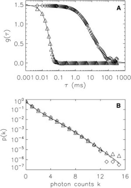
Comparison between flow- and stationary-FFS. A sample of spheres of 100-nm diameter at a concentration of 1.5 nM was measured with and without flow at a sampling frequency of 200 kHz for 20 s. (A) The autocorrelation functions for stationary (diamonds) and flowing (triangles) samples are fit as explained in the text. A diffusion coefficient of 2.8 μm²/s was determined for the spheres of the stationary sample. The flowing sample yielded a flow speed of 9 mm/s. The fluctuation amplitudes, g(0), of the two samples were identical and correspond to a concentration of 1.5 nM. A brightness of 9.2 × 10⁵ cps was determined from g(0) and the average intensity. (B) The PCHs of the stationary (diamonds) and flowing (triangles) sample fall on top of each other. Each PCH was fit to a single species model (χ² of 0.9 and 1.3). The brightness and concentration of the stationary and flowing samples agree and correspond to c = 1.5 ± 0.1 nM and a brightness of (9.2 ± 0.6) × 10⁵ cps/sphere.

The PCH $p_k\left(k\right)$ values for the flowing and stationary samples are identical within experimental uncertainty (Fig. 1 B). Thus, the brightness and concentration determined by PCH analysis are independent of flow. This result verifies that the probability distribution of the photon counts and its moments are independent of flow, as discussed in the Theory section. Consequently, the fluctuation amplitudes, g(0), for the flowing and stationary sample also have to be identical to those observed experimentally (Fig. 1 A).

Event sampling for flow- and stationary-FFS

Fluorescence fluctuation experiments were carried out on a stationary sample with fluorescent microspheres (diameter 100 nm) at low concentrations (110 fM). Data was collected for 160 s at 200 kHz. The intensity trace (Fig. S1 A in the Supporting Material) exhibits one spike, indicating the passage of one sphere during the experiment. This result is consistent with an event rate of ∼1/1800 s⁻¹ determined by Eq. 2, with D = 2.8 μm²/s, c = 110 fM, and R_O ≈ 1 μm. It is clear that the number of events is insufficient for FFS analysis. It would take approximately two days of measurement time to acquire the minimum sampling population for FFS analysis (∼100 events). By applying flow to the sample, the number of events greatly increases, as seen by the intensity trace (Fig. S1 B). Data were collected for 160 s with a flow speed of 8.7 mm/s. The event rate for the flowing sample (Eq. 3) is ∼2 s⁻¹, which is more than a 1000-fold increase compared to the stationary sample. The data collected for 160 s contains more than 100 events, which is sufficient for FFS analysis. The autocorrelation and PCH curve are shown in Fig. 2 and will be discussed further below. These experimental curves are reproducible when repeating the measurement (data not shown), which indicates that adequate sampling is achieved by the experiment.

Figure 2.

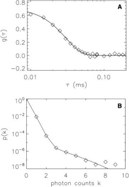
Flow-FFS of a low-concentration sample. Fluorescent spheres of 100-nm diameter at a concentration of 110 fM were measured for 160 s at a flow speed of ∼9 mm/s and a sampling frequency of 200 kHz. (A). The autocorrelation function of flowing spheres is shown together with the fit to the theoretical model. The flow time corresponds to a velocity of 8.7 mm/s which is in agreement with the expected value. However, the fluctuation amplitude, g(0), differs from the expected value by a factor of >1000, because background dominates. (B). PCH analysis of a flowing sample is plotted with a two-species fit. The first species identifies the background, which has a very low brightness, contributes 99.3% of the counts, and is the main source for the PCH, with k ≤ 3. The second species models the rare but bright spheres, and is represented by the tail section of the PCH curve. The fit returns a brightness of ∼10⁶ cps/sphere and a concentration of 107 fM, which agrees with the expected value based on the dilution factor.

The effect of background on FFS analysis

The autocorrelation function is fit to a flow-only model (Fig. 2 A, solid line) with a flow time of 30 μs, which agrees with a flow speed of 8.7 mm/s. However, the value of the fluctuation amplitude, $g\left(0\right)\approx 0.7$, corresponds to a concentration of 3 nM, which is inconsistent with the expected value of 110 fM. We will address this discrepancy after discussing the PCH function. The PCH function (Fig. 2 B) displays two distinct slopes pointing toward the presence of two brightness species. One slope is steep and occurs at photon count k < 3, which likely corresponds to a dim fluorescent background from the sample. The second slope is less steep and extends to large photon count numbers, as expected for bright particles. A single species fit fails to describe the PCH function, but a two-species PCH fit (reduced χ² = 0.9) reproduces the experimental curve (Fig. 2 B). The first species has λ_S = 1.03 × 10⁶ cps and N_S = 9.28 × 10⁻⁶, which corresponds to a concentration of 107 fM, in good agreement with the expected value of 110 fM. The second species has a much lower brightness (λ_B = 157 cps) and a higher concentration (N_B = 11.44) than the first species and therefore describes the background.

Note that according to PCH analysis, the intensity of the background ($F_{\text{B}}={\lambda }_{\text{B}}{N}_{\text{B}}$) is ∼1800 cps, whereas the fluorescent spheres only contribute an intensity ($F_{\text{S}}={\lambda }_{\text{S}}{N}_{\text{S}}$) of ∼10 cps to the fluorescence of the sample. We will use subscripts B and S for the background and sample, respectively. Let us evaluate briefly the influence of background on FFS data. The autocorrelation function, $g_{\text{F}}\left(\tau \right)$, of the sphere sample in the presence of background is (16,18)

$$g_{\text{F}}\left(\tau \right)={\left(\frac{F_{\text{S}}}{F_{\text{S}}+F_{\text{B}}}\right)}^2{g}_{\text{S}}\left(0\right)f_{\text{F}}\left(\tau \right)+{\left(\frac{F_{\text{B}}}{F_{\text{S}}+F_{\text{B}}}\right)}^2{g}_{\text{B}}\left(0\right)f_{\text{F}}\left(\tau \right).$$ (5)

Without background, the fluctuation amplitude of the sample would be $g_{\text{F}}\left(\tau \right)=g_{\text{S}}\left(0\right)$. The presence of a dim background leads to a suppression of the fluctuation amplitude, $g_{\text{F}}\left(\tau \right)<g_{\text{S}}\left(0\right)$. In fact, if we insert the PCH fit parameters into Eq. 4 with$g_i\left(0\right)={\gamma }_2/N_i$, we get 0.6, which is in close agreement with the experimentally measured fluctuation amplitude of 0.7 (Fig. 2 A). In other words, background fluorescence is responsible for the reduction of the fluctuation amplitude, which leads to incorrect brightness and concentration values. Thus, PCH analysis can be used to correct the influence of background on the g(0) value.

Note that it is impossible to separate the background contribution from the sample by autocorrelation analysis, because temporal correlations induced by background and sample are identical for flow-dominated conditions. This point will be discussed in more detail later. Although the temporal correlations are identical, the brightness of the background is much less than for the sample spheres. PCH exploits the brightness contrast to separate the background signal from the sample. Because background becomes a significant factor for ultralow sample concentrations, we will rely for the rest of this article on the remarkable ability of PCH to distinguish sample from background. We have found that the brightness of the background of all samples studied in this article is sufficiently low, so that the PCH of the background is indistinguishable from a Poisson distribution. Thus, the experimental PCH is well approximated by convoluting the PCH from the particles with a Poisson distribution for the background.

The effect of flow velocity on brightness and concentration

As mentioned in the Theory section, the PCH, and therefore the brightness and concentration, are not affected by flow speed as long as undersampling is avoided. Here, we verify this prediction experimentally by varying the flow speed of a sample containing 100 nm fluorescent microspheres at 1.5 nM concentration. All measurements are performed at a sampling frequency of 200 kHz (T = 5 μs). The speed was varied by changing the flow rate of the syringe pump, and the flow velocity was measured using autocorrelation analysis. We also measured a stationary sample ($v_{\text{F}}=0$). The brightness and concentration for each run was determined from a single-species PCH fit, as the background contribution was negligible. Fig. S2 demonstrates that brightness, λ, and occupation number, N, are constant for flow velocities ranging from 0 to 25 mm/s. However, undersampling leads to a reduction in the brightness and an increase in the concentration at a flow velocity of 44 mm/s (Fig. S2). Thus, the critical flow speed demarcating the onset of undersampling effects is between 25 and 44 mm/s, which corresponds to a flow time of ∼10 μs at a sampling time of T = 5 μs. Since undersampling depends on the flow and sampling time, their ratio provides a useful indicator for identifying undersampling conditions. Our experimental result shows that undersampling effects occur for ${\tau }_{\text{F}}/T<2$. We verified that this relationship remains valid for sampling times other than T = 5 μs (data not shown). In other words, PCH accurately determines the brightness and concentration, provided the data is sampled at least twice as fast as the flow time. All experiments presented in this article are conducted with ${\tau }_{\text{F}}/T\ge 2$.

Brightness versus concentrations of flowing particles

A dilution study was conducted on a flowing sample to evaluate the concentration range over which brightness and concentration are recovered by PCH analysis. A concentration of 100-nm spheres, which was initially 1.1 nM, was successively diluted 10-fold between measurements. Each sample from 1.1 nM to 1.1 pM was measured at the same flow speed for 1 min. The 110-fM sample was measured for 3 min, and the 11-fM sample was measured for 10 min. The increased measurement time was necessary to collect a sufficient number of events for statistical accuracy. When necessary, the PCH was analyzed with a two-species model to separate the sample brightness and concentration from the background fluorescence. Fig. 3 A shows that brightness is independent of sphere concentration, as expected. In addition, the fitted occupation number, N_S, is linear with concentration (Fig. 3 B). Experiments cover the concentration range from 1.1 nM down to 11 fM. Although it is possible to measure at concentrations lower than 11 fM, the associated reduction in the event rate requires either longer measurement times or higher flow rates to ensure adequate sampling for statistical analysis of the data.

Figure 3.

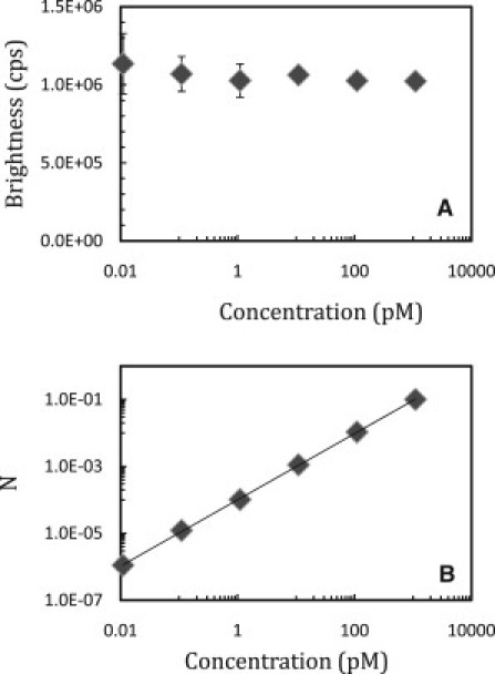
Serial dilution study of fluorescent spheres by flow-FFS. A sample of 100-nm fluorescent spheres at an initial concentration of 1.1 nM was successively diluted by factors of 10 and measured at a sampling frequency of 200 kHz and a flow velocity of ∼5 mm/s. The measurement time was increased with decreasing concentration. Concentrations down to 1.1 pM were measured for 1 min. At 110 fM and 11 fM the sample was measured for 3 min and 10 min, respectively. PCH analysis determined the brightness and occupation number of the spheres. (A) The brightness of the spheres remains constant. (B) The occupation number, N, scales linearly with concentration as expected. The error was determined from the standard deviation of multiple measurements at each concentration (n = 6, except in the case of 11 fM, where n = 3). Error bars are not visible if the symbol size is larger than the error.

Brightness and Gag copy number of VLPs

In the past, our lab has prepared HIV-1 VLPs containing YFP-tagged Gag and performed stationary-FFS measurements to determine the stoichiometry of the YFP-labeled Gag within the VLPs (11). These measurements present a significant challenge because of the low event rate due to low concentrations and slow diffusion. The measurement time required to collect a sufficient number of events ranged from 30 to 60 min. Applying flow-FFS should significantly shorten the measurement time and simultaneously increase the number of events.

Flow experiments were performed on a 10-fold concentrated VLP sample. The brightness of monomeric YFP was measured for calibration at the center of the channel as previously described (11). The channel was then rinsed with phosphate-buffered saline (PBS) and the concentrated VLP solution was loaded. Pressure-driven flow was used to obtain a flow rate of ∼2 mm/s. This flow rate results in an ∼150× increase in the number of events compared to stationary-FFS. Measurements were taken at 20 kHz for 80 s. Autocorrelation analysis was performed to determine the flow velocity to ensure that undersampling is avoided. The PCH of the data was fit to a single brightness species model with a Poissonian background. However, this model is insufficient to describe the data (reduced χ² > 20), which indicates the presence of brightness heterogeneity of the VLP sample. We added a second brightness species to the model, which resulted in a good description (reduced χ² < 2) of the data (Fig. 4). The majority of photon counts with k < 3 account for the background, which contributes ∼90% of the signal, whereas the long tail at low p(k) represents the VLP signal. Our result agrees with the published stationary-FFS study, which also identified two brightness species (11). The two brightness species were interpreted as an approximation of a brightness distribution of the VLP sample by the PCH fit. Thus, the two brightness species point toward a distribution of Gag copy numbers of the VLP sample. The previous study also observed that changing the amount of plasmid used in the transfection of cells resulted in brightness changes of the VLPs. A higher amount of plasmid resulted in increased brightness values for the two species, which reflects a change in the Gag copy number distribution. We confirmed this dependence of the two brightness species on the amount of transfected plasmid by flow-FFS (data not shown).

Figure 4.

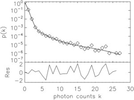
PCH of flowing VLPs. HIV-1 VLPs collected from cos-1 cells transfected with 2.1 μg of DNA and concentrated in PBS were measured at a flow velocity of 2.2 mm/s for 50 s at a sampling frequency of 20 kHz. (Upper) The PCH (diamonds) and fit (line) to a two-species model with Poissonian background (χ² = 1.1). (Lower) Normalized residuals of the fit. The background contributes 88% of the photon counts and dominates the PCH for k ≤ 3. The VLP events are captured by the long tail of the PCH curve. The first brightness species corresponds to a Gag copy number of 1300 with a concentration of 20 pM. The second brightness species corresponds to a copy number of 3900 and a concentration of 3 pM.

Because the properties of the VLPs depend on the sample preparation conditions, a direct comparison between this and the former study is difficult. We therefore performed stationary VLP measurements in addition to flow-FFS on the same sample to directly compare the two methods. A 10-fold concentrated VLP sample was measured by flow-FFS with a flow speed of 2 mm/s for 80 s at 20 kHz. A two-species fit with Poissonian background describes the PCH data within experimental uncertainty. The uncertainty of the fit parameters was established by repeated measurements (n = 5) of the same sample. Gag copy numbers of the two fitted species are determined from the normalized brightness, as described in the Materials and Methods section. Next, the same 10-fold concentrated sample was measured in the absence of flow for 30 min at 20 kHz. Autocorrelation analysis returned a diffusion time that corresponds to a VLP diameter of 130 ± 10 nm, in agreement with previously reported numbers (11). PCH analysis required two brightness species with a Poissonian background to describe the experiment. The Gag copy numbers and concentration of the stationary and flow-FFS measurements agree with one another (Table 1).

Table 1.

Gag copy number and concentration of VLPs

Sample preparation	Acquisition time (s)	Gag copy No., species 1	Gag copy No., species 2	Concentration, species 1 (pM)	Concentration, species 2 (pM)
10× concentrated, PBS, stationary	1800	1370 ± 400	4000 ± 1000	16 ± 4	3.0 ± 1.5
10× concentrated, PBS, flowing	50	1320 ± 100	4200 ±  400	18 ± 3	3.0 ± 0.5
1× concentrated, cell medium, flowing	160	1350 ± 200	4000 ± 600	2.0 ± 0.4	0.4 ± 0.2

HIV-1 VLPs were collected from the supernatant of cos-1 cells. The 10-fold concentrated sample was measured multiple times (n = 5) with and without flow. In addition, FFS measurements (n =5) were also performed directly on the unconcentrated cell supernatant. FFS analysis determined the concentration and Gag copy numbers together with their standard deviations. The table also lists the data acquisition time. Flow greatly reduces the measurement time, at the same time returning FFS results in agreement with stationary measurements.

The cell supernatant contains VLPs, which are subsequently concentrated 10-fold into PBS. To test whether it is possible to avoid the time-consuming concentration step, we measured the cell supernatant by flow-FFS. The cell medium of the supernatant presents a challenge as the background can be greatly increased from the concentrated sample. For the medium tested (DMEM without phenol red), the background intensity increased by a factor of ∼3 from the concentrated sample. The VLPs in cell medium were measured under flow (v_F = 2 mm/s) at 20 kHz with a collection time of 160 s. Autocorrelation and PCH analysis were performed as described above. Again, a two-species model with Poissonian background was required to fit the PCH data. The copy numbers agreed with the values obtained for the 10-fold concentrated sample (Table 1). The concentrations of the original and concentrated samples differed by a factor of ∼10, at the same time retaining the same concentration relationship between the two VLP species. Measurements of nonconcentrated VLPs in cell medium were also performed for different types of cell medium, including DMEM with phenol red. Although phenol red increases the background counts by a factor of 10, the copy numbers and concentration returned were consistent with measurements of samples concentrated into PBS. Taken together, our results indicate that characterization of VLPs by flow-FFS not only is feasible, but also offers significant advantages over stationary-FFS. VLPs can be measured directly in cell supernatant without concentrating the sample, using much shorter data acquisition times than required for stationary-FFS.

Discussion

The experimental results establish that flow-FFS offers significant advantages over conventional FFS of bright biomolecular particles at low concentrations. Here, we briefly discuss the main factors that need to be considered in flow-FFS. Flow increases the event rate of particle detection, which is widely exploited for the measurement of samples at low concentrations. However, even in the presence of flow, FCS experiments of bright particles at low concentrations remain challenging because of background fluorescence. Because flow-dominated FCS cannot distinguish particles from background, an independent FCS measurement of the background could potentially serve as a calibration, which may be used to correct the sample from the background effect. Unfortunately, even if it is possible to prepare a calibration sample for the background, this experimental strategy is, from a practical point of view, impossible. To illustrate the problem consider a sample with 1050 cps. If the background from the calibration sample is 1000 cps, then 50 cps are by calibration from the bright particles, which leads to a correction factor for g(0) of 440. However, let us assume that the actual background of the sample is 1040 cps, which just differs from the calibration sample by 4%. The correction factor for g(0) is now 11,000. Thus, 4% uncertainty in the background signal leads to a 25-fold difference in estimating g(0). Because of the inherent variability of biological sample preparations and the slight variations from measurement to measurement, it is clear that the required accuracy of the calibration approach cannot be achieved.

Because it is currently impossible to incorporate background into the analysis of sparse but bright particles, an alternative analysis was introduced that is based on fluorescent peak detection and uses a threshold to distinguish signal from background (12,19,20). Although it has been shown that the particle concentration is proportional to the area under the peaks, quantitative modeling of the peaks is still under development and brightness analysis is not yet feasible.

This article introduces the first method capable of quantifying sparse but bright particles in the presence of background. PCH distinguishes background from particles by the shape of the photon-count distribution. Because the theory of PCH is known, the concentration and brightness of the particles is determined from an analysis of the photon count distribution. It is further possible to detect heterogeneity in the brightness of the fluorescent particles using PCH, as demonstrated for the VLP sample. Because PCH determines the background from a measurement of the actual sample, any uncertainty associated with a calibration measurement is avoided. PCH solves the problem associated with fluorescence background, and thereby provides quantitative interpretation of g(0), brightness, and concentration of bright particles at low concentrations.

Because we perform quantitative PCH, a minimum number of events are required for a statistically meaningful analysis. Although it is difficult to pinpoint the exact number of events necessary, the following observations might provide a useful starting point. We have found that a minimum of ∼100 events is suitable if the particles are of uniform brightness. However, in the presence of brightness heterogeneity, such as encountered for the VLPs, ∼1000 events are needed to identify two brightness species. The data acquisition time is determined by dividing the number of events by the event rate, which is proportional to the particle concentration and the flow speed. Thus, in our case it takes ∼5 min to acquire 100 events for a concentration of 10 fM at a flow speed of 20 mm/s.

It is tempting to increase the flow speed, because it reduces the data acquisition time. However, this approach is not suitable in the presence of a significant amount of background counts. To illustrate the problem, consider particles at a concentration of 1 pM (N = 8 × 10⁻⁵). Each particle carries 500 copies of YFP, and each YFP has a brightness of 300 cps. Although the brightness of the particle is 150,000 cps, the intensity of the particles is only ∼10 cps. If the background is 1000 cps, the background constitutes 99% of the measured signal (f_B = 0.99). PCH needs to separate the signal of the particles from the background. For this to occur, the presence of the fluorescent particles has to add a component to the PCH that clearly distinguishes it from Poisson-background. Here, the sampling time becomes important, because deviation from the Poisson distribution depends on ɛ, which in the absence of undersampling is given by $\varepsilon =\lambda T$ (6). To maximize ɛ, it is necessary to select the longest sampling time that avoids undersampling, which for flow is $T={\tau }_{\text{F}}/2$. Thus, the maximum photon counts/particle depends on the flow speed ($\varepsilon =\lambda {\tau }_{\text{F}}/2$), which leads to a trade-off between maximizing ɛ and minimizing the data acquisition time.

The significance of ɛ becomes apparent by continuing to examine our earlier example of particles with brightness of 150,000 cps at a concentration of 1 pM with 1000 cps from background. A flow speed of 2 mm/s leads to an optimal sampling frequency of 20 kHz, which implies a mean of $\langle k\rangle =0.05$ for the Poissonian background and ɛ = 7.5 for the particles. We modeled the PCH of this sample (Fig. 5, squares). The deviation from the Poisson of the background (Fig. 5, dashed line) is evident and ensures a clean identification of the particle properties by PCH analysis. Now consider a 10-fold increase in the flow speed. The sampling frequency increases to 200 kHz, which results in $\langle k\rangle =0.005$ for the background and ɛ = 0.75 for the particles. The modeled PCH of the sample (diamonds) is now almost indistinguishable from the Poissonian background (Fig. 5, dashed line). This example demonstrates the importance of the photon counts per sampling time, ɛ, for separating the particle signal from the background. The parameters chosen in this example are close to the actual parameters found in the VLP experiments, which explains why a flow speed of 2 mm/s was adopted for our measurements. The minimum value of ɛ required for characterizing particles depends on the background level, the particle concentration, and the data acquisition time. The appropriate value for ɛ is best discovered by performing the same type of modeling as discussed above (see Fig. 5) using estimated parameters for the brightness and background counts of the system in question. As a rule of thumb, ɛ > 1 is typically required to distinguish the sample from the Poissonian background.

Figure 5.

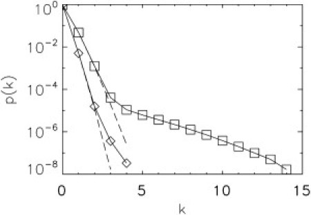
Modeled PCH curve at two sampling frequencies. The PCH for particles with a brightness of 1.5 × 10⁵ cps at 1 pM concentration (N = 8 × 10⁻⁵) in the presence of a Poissonian background of 1000 cps were modeled for two different sampling frequencies. The PCH (squares) for a sampling frequency of 20 kHz provides a clear separation of the sample from the Poissonian background (dashed line). However, a sampling frequency of 200 kHz results in a PCH (diamonds) that is almost indistinguishable from the Poissonian background (dashed line). Thus, successful separation between sample and background by PCH requires careful consideration of the sampling frequency (for details, see text).

Although the average intensity of the flowing sample is very low, the passage of a particle results in a spike of the intensity. These transient intensities are high enough that deadtime and afterpulsing artifacts of the detector need to be taken into account in PCH analysis (14). In addition, the peak intensities may be high enough to saturate the detector, which in our case occurs at ∼10⁷ cps. In fact, experimental conditions where the VLP and microspheres lead to saturation are easy to achieve, and we have encountered such cases in our work. Under saturating conditions, the PCH curve $p\left(k\right)$ exhibits a cutoff in k, which corresponds to the saturating intensity. In addition, the measured PCH deviates significantly from the model function. We avoid saturation by reducing the excitation power at the sample. In this article, we choose conditions where the maximum photon count, k_Max = F_LimitT, observed in the PCH function corresponds to intensities of no more than F_Limit = 2 × 10⁶ cps. Because the PCH correction algorithms for deadtime and afterpulsing have previously been tested up to intensities of 2 × 10⁶ cps (21), the PCH analysis of flowing particles is expected to be free of systematic artifacts. As an additional test, we measured a flowing sample as a function of excitation power and calculated its brightness and concentration by PCH analysis. For peak intensities up to 2 × 10⁶ cps, the brightness scaled with the square of the excitation power, whereas the concentration remained constant (data not shown). This result confirms that under our experimental conditions, PCH analysis is well behaved.

As mentioned earlier, flow together with fluorescence peak analysis has been used to detect bright particles at low concentrations and estimate their concentration. A distinct advantage of flow-FFS is the ability to not only measure the concentration, but also provide information about the protein copy number of rare but bright particles. Our earlier study of HIV-1 VLPs by stationary-FFS established that the Gag copy number of VLPs is heterogeneous and depends on the sample preparation conditions. The reason for this complex behavior of Gag stoichiometry is not currently understood and requires further investigation. In the past, every VLP sample had to be concentrated 10-fold to reduce the minimum acquisition time required for PCH analysis to 30 min. The time-consuming procedure of preparing and measuring VLPs severely limits our ability to systematically investigate the factors that influence Gag stoichiometry. We have shown that flow-FFS provides the same information regarding Gag stoichiometry as stationary-FFS, but in <5 min of measurement time and without concentrating the sample. Thus, flow-FFS presents an attractive alternative for the future characterization of VLP stoichiometry. The only disadvantage of flow-FFS compared to stationary-FFS is the lack of information regarding diffusion, which is useful for determining the size of VLPs.

The highest Gag copy number achieved in the previous study of HIV-1 VLPs is ∼2500, whereas theory predicts a maximum of 4000–5000 (11). In this article, we not only increased the statistical accuracy of the results, but also succeeded in measuring copy numbers that approach the theoretical limit. The variability in Gag copy number with sample preparation requires further study. Note that relating brightness and copy number assumes the absence of fluorescence quenching in the VLP particles. This has been confirmed by a series of experiments described in the original publication (11).

Although this article focused on viral particles, flow-FFS is suitable for the characterization of any bright fluorescent particle, provided it contains a sufficient number of fluorescent labels. With our current setup, ∼50 YFP-labeled proteins/particle are needed to separate signal from background at picomolar concentrations, but further technical improvements might increase the sensitivity of the technique. Particle size is another factor that needs to be considered. The VLPs are small enough that their finite size can be ignored in FFS analysis. However, particles that approach the size of the observation volume require analysis models that take size into account (17).

We have shown that flow-FFS accurately determines the brightness and concentration of particles at low concentrations. This study has successfully employed flow-FFS on concentrations as low as 10 fM. Furthermore, we have shown that measurement of rare but bright particles requires flow, which increases the event rate of particle detection, and PCH analysis, which separates the particle signal from background. This article contains detailed information on selecting experimental parameters and provides guidelines for conducting flow-FFS experiments. We emphasize that brightness is a unique parameter, because it identifies the copy number of labeled proteins within a particle. Specifically, we determine the HIV-1 Gag copy number of VLPs at picomolar concentration. This work demonstrates that flow-FFS is a promising method for extracting quantitative information about the composition of large supramolecular complexes.

References

- 1.Elliot L.E., Douglas M. Fluorescence correlation spectroscopy. I. Conceptual basis and theory. Biopolymers. 1974;13:1–27. [Google Scholar]
- 2.Thompson N.L., Lieto A.M., Allen N.W. Recent advances in fluorescence correlation spectroscopy. Curr. Opin. Struct. Biol. 2002;12:634–641. doi: 10.1016/s0959-440x(02)00368-8. [DOI] [PubMed] [Google Scholar]
- 3.Schwille P. Fluorescence correlation spectroscopy and its potential for intracellular applications. Cell Biochem. Biophys. 2001;34:383–408. doi: 10.1385/CBB:34:3:383. [DOI] [PubMed] [Google Scholar]
- 4.Chen Y., Müller J.D., Gratton E. The photon counting histogram in fluorescence fluctuation spectroscopy. Biophys. J. 1999;77:553–567. doi: 10.1016/S0006-3495(99)76912-2. [DOI] [PMC free article] [PubMed] [Google Scholar]
- 5.Kask P., Palo K., Gall K. Fluorescence-intensity distribution analysis and its application in biomolecular detection technology. Proc. Natl. Acad. Sci. USA. 1999;96:13756–13761. doi: 10.1073/pnas.96.24.13756. [DOI] [PMC free article] [PubMed] [Google Scholar]
- 6.Müller J.D. Cumulant analysis in fluorescence fluctuation spectroscopy. Biophys. J. 2004;86:3981–3992. doi: 10.1529/biophysj.103.037887. [DOI] [PMC free article] [PubMed] [Google Scholar]
- 7.Chen Y., Wei L.-N., Müller J.D. Probing protein oligomerization in living cells with fluorescence fluctuation spectroscopy. Proc. Natl. Acad. Sci. USA. 2003;100:15492–15497. doi: 10.1073/pnas.2533045100. [DOI] [PMC free article] [PubMed] [Google Scholar]
- 8.Chen Y., Müller J.D. Determining the stoichiometry of protein heterocomplexes in living cells with fluorescence fluctuation spectroscopy. Proc. Natl. Acad. Sci. USA. 2007;104:3147–3152. doi: 10.1073/pnas.0606557104. [DOI] [PMC free article] [PubMed] [Google Scholar]
- 9.Wu B., Chen Y., Müller J.D. Heterospecies partition analysis reveals binding curve and stoichiometry of protein interactions in living cells. Proc. Natl. Acad. Sci. USA. 2010;107:4117–4122. doi: 10.1073/pnas.0905670107. [DOI] [PMC free article] [PubMed] [Google Scholar]
- 10.Duckworth B.P., Chen Y., Distefano M.D. A universal method for the preparation of covalent protein-DNA conjugates for use in creating protein nanostructures. Angew. Chem. Int. Ed. 2007;46:8819–8822. doi: 10.1002/anie.200701942. [DOI] [PubMed] [Google Scholar]
- 11.Chen Y., Wu B., Mueller J.D. Fluorescence fluctuation spectroscopy on viral-like particles reveals variable gag stoichiometry. Biophys. J. 2009;96:1961–1969. doi: 10.1016/j.bpj.2008.10.067. [DOI] [PMC free article] [PubMed] [Google Scholar]
- 12.Bieschke J., Giese A., Kretzschmar H. Ultrasensitive detection of pathological prion protein aggregates by dual-color scanning for intensely fluorescent targets. Proc. Natl. Acad. Sci. USA. 2000;97:5468–5473. doi: 10.1073/pnas.97.10.5468. [DOI] [PMC free article] [PubMed] [Google Scholar]
- 13.Magde, D., W. Webb, and E. Elson, L. 1978. Fluorescence correlation spectroscopy. III. Uniform translation and laminar flow. Biopolymers. 17: 361–376 [DOI] [PubMed]
- 14.Hillesheim L.N., Müller J.D. The photon counting histogram in fluorescence fluctuation spectroscopy with non-ideal photodetectors. Biophys. J. 2003;85:1948–1958. doi: 10.1016/S0006-3495(03)74622-0. [DOI] [PMC free article] [PubMed] [Google Scholar]
- 15.Müller J.D., Chen Y., Gratton E. Resolving heterogeneity on the single molecular level with the photon-counting histogram. Biophys. J. 2000;78:474–486. doi: 10.1016/S0006-3495(00)76610-0. [DOI] [PMC free article] [PubMed] [Google Scholar]
- 16.Thompson N.L. Fluorescence correlation spectroscopy. In: Lakowicz J.R., editor. Topics in Fluorescence Spectroscopy. Plenum; New York: 1991. pp. 337–378. [Google Scholar]
- 17.Wu B., Chen Y., Müller J.D. Fluorescence correlation spectroscopy of finite-sized particles. Biophys. J. 2008;94:2800–2808. doi: 10.1529/biophysj.107.112789. [DOI] [PMC free article] [PubMed] [Google Scholar]
- 18.Chen Y., Müller J.D., Gratton E. Probing ligand protein binding equilibria with fluorescence fluctuation spectroscopy. Biophys. J. 2000;79:1074–1084. doi: 10.1016/S0006-3495(00)76361-2. [DOI] [PMC free article] [PubMed] [Google Scholar]
- 19.Perevoshchikova I.V., Zorov D.B., Antonenko Y.N. Peak intensity analysis as a method for estimation of fluorescent probe binding to artificial and natural nanoparticles: tetramethylrhodamine uptake by isolated mitochondria. Biochim. Biophys. Acta. 2008;1778:2182–2190. doi: 10.1016/j.bbamem.2008.04.008. [DOI] [PubMed] [Google Scholar]
- 20.Van Craenenbroeck E., Matthys G., Engelborghs Y. A statistical analysis of fluorescence correlation data. J. Fluoresc. 1999;9:325–331. [Google Scholar]
- 21.Sanchez-Andres A., Chen Y., Müller J.D. Molecular brightness determined from a generalized form of Mandel's Q-parameter. Biophys. J. 2005;89:3531–3547. doi: 10.1529/biophysj.105.067082. [DOI] [PMC free article] [PubMed] [Google Scholar]
Associated Data
This section collects any data citations, data availability statements, or supplementary materials included in this article.