An Adaptive Expectation-Maximization Algorithm with GPU Implementation for Electron Cryomicroscopy

Abstract

Maximum-likelihood (ML) estimation has very desirable properties for reconstructing 3D volumes from noisy cryo-EM images of single macromolecular particles. Current implementations of ML estimation make use of the Expectation-Maximization (EM) algorithm or its variants. However, the EM algorithm is notoriously computation-intensive, as it involves integrals over all orientations and positions for each particle image. We present a strategy to speed up the EM algorithm using domain reduction. Domain reduction uses a coarse grid to evaluate regions in the integration domain that contribute most to the integral. The integral is evaluated with a fine grid in these regions. In the simulations reported in this paper, domain reduction gives speedups which exceed a factor of 10 in early iterations and which exceed a factor of 60 in terminal iterations.

1 Introduction

Single-particle reconstruction is the process by which noisy two-dimensional images of individual, randomly-oriented macromolecular “particles” are used to determine one or more three-dimensional electron-scattering-density “maps” of the underlying macromolecules. All of the algorithms that perform such reconstructions are iterative. Each iteration begins with a guess of the particle structure, then aligns the cryo-EM images with the structure, and averages the aligned images to update the structure. The alignment step is especially critical in overcoming noise and improving resolution.

For the alignment step, traditional algorithms choose the best alignment to the current guess of the structure. This “best alignment” strategy is simple to implement, but can be troublesome when used with noisy images because noisy images can match at wrong alignments. The problem is that the “best alignment” strategy ignores alignments that are almost as good as – but are not – the best alignment.

One class of reconstruction algorithms which does not have this limitation is based on the maximum-likelihood (ML) principle. These algorithms do not use the best alignment for structure update, but instead use the Expectation-Maximization (EM) algorithm or variants thereof, which form a weighted average over all alignments for the structure update. The weighted averaging allows the non-best-match alignments to contribute. In cryo-EM, the ML principle was proposed for 2D image restoration [13] and subsequently generalized to the estimation of multiple image classes [11] and for the optimization of unit-cell alignment in images of crystals [17]. The ML principle has also been extended to the problem of 3D reconstruction from 2D cryo-EM images by [15, 16, 11, 5, 12, 10].

Even though it has appealing properties, the EM algorithm has a limitation: it is computationally slow. Calculating the expectation over all alignments (i.e. averaging over all alignments) is expensive and the EM algorithm can easily take CPU-months to converge. In this paper, we report two strategies for speeding up the EM algorithm for cryo-EM. The first strategy is based on the work of Sander et al. [8] and speeds up the EM algorithm by computing the expectation only over those alignments that contribute significantly to the weighted average. This is the “adaptive” part of our algorithm. Our experiments show that it significantly speeds up the EM algorithm without losing accuracy. The second strategy is the use of graphics processing units (GPUs) to accelerate the most computation-intensive parts of the calculations.

To put previous attempts to speed up the EM algorithm in context, we first explain the basic EM iteration. The EM iteration has two steps, in the the first step the latent data probability is calculated and in the second step this probability is used for calculating the weighted averages. Both calculations involve integration over all possible alignments and contribute equally to the computational complexity.

Previous attempts to speed up the EM algorithm can be classified into two groups. The first group of algorithms uses spherical harmonics as basis functions for the structure [15, 16, 5]. These algorithms have the computational advantage that integrations with respect to rotations can be calculated in closed form. However, integration with respect to translations still need to calculated numerically. The second group contains the algorithm of Scheres et. al. [11] and is similar in its approach to our algorithm. This algorithm decreases computational cost by calculating the EM integrals over a smaller integration domain. Scheres et al.’s strategy is quite complex: The first EM iteration is carried out in its entirety over alignments. For all subsequent iterations, every image is compared with every class mean using the most significant translations from the previous iteration for this pair. Using these translations, the latent probability that the image comes from that class is calculated for every rotation. All rotations for which the calculated probability exceeds a fraction of the maximum value of all calculated probabilities are retained. The EM integration is carried out over alignments formed by the surviving rotations and all translations.

One problem with this strategy is that it is not entirely clear whether thresholding the probability to reduce the domain gives good approximations to the integral. If the domain of integration is to be reduced, then the reduction strategy ought to be based on how changing the domain affects the integral rather than on thresholding a function. Our algorithm includes such a strategy, and is inspired by adaptive integration techniques in numerical analysis [1]. We first use a coarse grid to estimate the contribution to the integral at every alignment. Then, we retain the smallest set of alignments over which the integral contributes a fraction (e.g. 0.999) of the net integral.

2 The ML formulation

Suppose that μ is a projection of a structure along a specific direction. An observed cryo-EM image I is μ with additive noise and a random in-plane rotation and shift. Letting T_τ represent the in-plane image rotation and translation operator, where τ = (θ, t_x, t_y) is the rotation and translation, the observed image is I = T_τ (μ + n), or, T_−τ (I) = μ + n, where, n is additive white Gaussian noise. Thus the probability density function (pdf) of observing an image I is

$$p(I\mid \mu ,\sigma )={\int }_{\Omega }{p}_g\left(T_{-\tau }\right(I)\mid \mu ,\sigma )p\left(\tau \right)d\tau ,$$ (1)

where, p(τ) is the density of τ, Ω is the support of p(τ ), and

$$p_g\left(T_{-\tau }\right(I)\mid \mu ,\sigma )=\frac{1}{{\left(2\pi {\sigma }^2\right)}^{P∕2}}\times \exp (-\frac{{\Vert T_{-\tau }\left(I\right)-\mu \Vert }^2}{2{\sigma }^2}),$$ (2)

where, ∥ ∥ is the usual Euclidean norm, P is the number of pixels in the image, and σ² is the noise variance of each pixel. The support Ω = [0, 2π) × [−t_max, t_max] × [−t_max, t_max] for some maximum translation t_max.

A small aside to emphasize an important point – typically in equation (2) the value of ∥T_−τ (I)–μ∥² is several orders of magnitude larger than the value of σ² (the former is the pixel-wise squared difference summed over the entire image while the latter is the noise variance of a single pixel). Because small changes in ∥T_−τ (I) – μ∥² are vastly amplified by the exponentiation, small changes in ∥T_−τ (I) – μ∥² can cause large changes in the value of p_g.

Cryo-EM obtains images from unknown random projection directions. It is common to model this phenomenon as follows: Let μ_j, j = 1, … ,M be the projection of the particle along the jth direction. Then, assuming that images are random draws from one of the projections, the pdf of an image I is

$$p(I\mid {\mu }_1,\cdots ,{\mu }_M,\sigma ,{\alpha }_1,\cdots ,{\alpha }_M)=\sum _{j=1}^M{\alpha }_{j}p(I\mid {\mu }_j,\sigma ),$$ (3)

where, the coefficients α_j are non-negative and sum to 1, and the densities p(I ∣ μ_j, σ) are given by equation (1) with μ = μ_j. This probability density model is popularly called a mixture model. The densities p(I ∣ μ_j, σ) are called class densities and the coefficients α_j are called mixture coefficients. The means μ_j are called class means.

Suppose that N images I_k, k = 1, … ,N are obtained in this way. Then, the joint density of the images is

$$p(I_1,\dots ,I_N\mid {\mu }_1,\cdots ,{\mu }_M,\sigma ,{\alpha }_1,\cdots ,{\alpha }_M)=\prod _{k=1}^{N}p(I_k\mid {\mu }_1,\cdots ,{\mu }_M,\sigma ,{\alpha }_1,\cdots ,{\alpha }_M).$$ (4)

A maximum-likelihood estimate of μ₁, … , μ_M, σ, α₁, … , α_M is given by

$$\begin{array}{cc}\hfill & \{{\widehat{\mu }}_1,\cdots ,{\widehat{\mu }}_M,\widehat{\sigma },{\widehat{\alpha }}_1,\cdots ,{\widehat{\alpha }}_M\}\hfill \\ \hfill =& \arg \underset{{\mu }_1,\cdots ,{\mu }_M,\sigma ,{\alpha }_1,\cdots ,{\alpha }_M}{\max }\log p(I_1,\dots ,I_N\mid {\mu }_1,\cdots ,{\mu }_M,\sigma ,{\alpha }_1,\cdots ,{\alpha }_M).\hfill \end{array}$$ (5)

2.1 The EM algorithm

The EM algorithm iteratively converges to the maximum-likelihood estimate of equation (5). The EM algorithm and its application to cryo-EM is not new. But we present some its details in order to motivate the adaptive-EM algorithm. The EM algorithm works by introducing additional random variables, called latent variables. For the maximum-likelihood problem of equation (5) the EM algorithm introduces two latent variables per image. Together they denote the component of and the transformation for the k^th image. For the k^th image the latent random variables are denoted y_k and τ_k. The variable y_k is a discrete valued random variable taking values y_k ∈ {1, … ,M} . The event y_k = j indicates that the k^th image comes from the j^th component. The random variable τ_k = ( θ_k, t_x,k, t_y,k) takes values τ_k ∈ Ω.

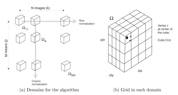
Because y_k takes values in y_k ∈ {1, … ,M} and τ_k in Ω, the joint random variable (y_k, τ_k) takes values in {1, … ,M} × Ω. In figure 1a, we show {1, … ,M} × Ω as a column of M × Ω domains. There are N such columns corresponding to N images. Below we will need to refer to the M × N copies of the domain Ω in figure 1a individually and collectively. We will refer to the domain in the j^th row and k^th column as Ω_jk. We will collectively refer to all domains as ʊ, i.e. ʊ = ∪_j,kΩ_jk.

Figure 1.

Structures for the EM algorithm.

The EM iterations proceed as given below. The superscripts [n – 1] and [n] refer to the values of the variables in the n – 1^st and n^th iteration:

The EM Algorithm

1. Initialize: Set n = 0 and initialize ${\alpha }_j^{\left[0\right]}$,${\mu }_j^{\left[0\right]}$ σ^[0] for j = 1, … ,M.

2. Start Iteration: Set n = n + 1.

3. Calculate Latent Probabilities: For all points in Ω_jk calculate

   $$p(y_k=j,{\tau }_k\mid I_k,{\theta }^{[n-1]})=\frac{{\alpha }_j^{[n-1]}{p}_g\left(T_{-{\tau }_k}\right(I_k)\mid {\mu }_j^{[n-1]},{\sigma }^{[n-1]})p\left({\tau }_k\right)}{\sum _{i=1}^M{\alpha }_i^{[n-1]}{\int }_{{\Omega }_{ik}}{p}_g\left(T_{-{\tau }_k}\right(I_k)\mid {\mu }_i^{[n-1]},{\sigma }^{[n-1]})p\left({\tau }_k\right)d{\tau }_k}.$$ (6)

   and

   $$\tilde{p}(y_k=j,{\tau }_k\mid I_k,{\theta }^{[n-1]})=\frac{p(y_k=j,{\tau }_k\mid I_k,{\theta }^{[n-1]})}{\sum _{i=1}^N{\int }_{{\Omega }_{ji}}p(y_i=j,{\tau }_i\mid I_i,{\theta }^{[n-1]})d{\tau }_i}.$$ (7)

   The variable i in the both denominators of the above formulae is a summation variable. In equation (6) the variable i sums over rows, and in equation (7) the variable i sums over columns.
4. Update Parameters: The parameter ${\alpha }_j^{\left[n\right]}$ is updated using the probability density p of equation (6)

   $${\alpha }_j^{\left[n\right]}=\frac{1}{N}\sum _{k=1}^N{\int }_{{\Omega }_{jk}}p(y_k=j,{\tau }_k\mid I_k,{\theta }^{[n-1]})d{\tau }_k.$$ (8)

   The parameters ${\mu }_j^{\left[n\right]}$, σ^[n] are updated using the density $\tilde{p}$ of equation (7):

   $${\mu }_j^{\left[n\right]}=\sum _{k=1}^N{\int }_{{\Omega }_{jk}}{T}_{-{\tau }_k}\left(I_k\right)\tilde{p}(y_k=j,{\tau }_k\mid I_k,{\theta }^{[n-1]})d{\tau }_k,$$ (9)

   and

   $${\left({\sigma }^2\right)}^{\left[n\right]}=\frac{1}{MP}\sum _{j=1}^M\sum _{k=1}^N{\int }_{{\Omega }_{jk}}{\Vert T_{-{\tau }_k}\left(I_k\right)-{\mu }_j^{[n-1]}\Vert }^2\tilde{p}(y_k=j,{\tau }_k\mid I_k,{\theta }^{[n-1]})d{\tau }_k.$$ (10)

   Note that the updates of μ and σ are weighted averages of T_−τk (I_k and ${\Vert T_{-{\tau }_k}\left(I_k\right)-{\mu }_j^{[n-1]}\Vert }^2$ with $\tilde{p}$ as the weight.

5. Loop: Stop if ${\alpha }_j^{\left[n\right]}$, ${\mu }_j^{\left[n\right]}$, σ^[n] have converged. Else go to step 2.

A useful visualization of the EM iterations is presented in figure 1a:

1. Begin by calculating ${\Vert T_{-{\tau }_k}\left(I_k\right)-{\mu }_j^{[n-1]}\Vert }^2$ in Ω_jk.

2. From this calculate ${\alpha }_k{p}_g\left(T_{-{\tau }_k}\right(I_k)\mid {\mu }_j^{[n-1]},{\sigma }^{[n-1]})p\left({\tau }_k\right)$ in every Ω_jk. Normalize this function column wise in ʊ so that the net integral of the function in each column is 1. This is illustrated in figure 1a and referred to as column normalization. The normalized function is the latent data probability of equation (6). The denominator in equation (6) achieves the normalization.

3. Next, normalize the function obtained in the above step so that its net integral in each row of ʊ is 1. This is also illustrated in figure 1a and called row normalization. The normalization is achieved by the denominator in equation (7). The result of row normalization is the function $\tilde{p}$.

4. Update μ_j and σ² according to equations (9-10) using weighted averages with $\tilde{p}$ as the weight.

3 Adaptive-EM

3.1 Speeding up the EM algorithm

The EM iteration described above is computationally expensive. Equations (6-10) require integration over the domains Ω_jk. These integrals are not available in closed form and have to be evaluated numerically. To do this, we introduce a grid in every Ω_jk (see fig. 1b) and approximate the integrals with a Riemann sum of the integrand over the vertices of the grid. The grid consists of cubes of size Δθ × Δt_x × Δt_y. The center of each cube is a vertex of the grid. We use v to refer to a vertex, and C(v) to refer to its cube.

The computationally expensive part of the algorithm is the calculation of the ${\Vert T_{-{\tau }_k}\left(I_k\right)-{\mu }_j^{[n-1]}\Vert }^2$ term at each vertex of the grid. We employ two strategies to speed up the EM iteration. Both strategies require various formulae in equations (6-10) to be approximated. The first strategy is called domain reduction and it replaces the integration over Ω_jk with integration over smaller subsets. The second strategy is called grid interpolation and uses two grids – a coarse grid for estimating the reduced domain, and a fine grid in the reduced domain for calculating the formulae. Analogous strategies have been used by Sander et al. [8] for angular search in a conventional reconstruction algorithm. The difference is that our strategy is for approximating an integral whereas Sander et. al.’s strategy is for approximating a maximum-seeking search.

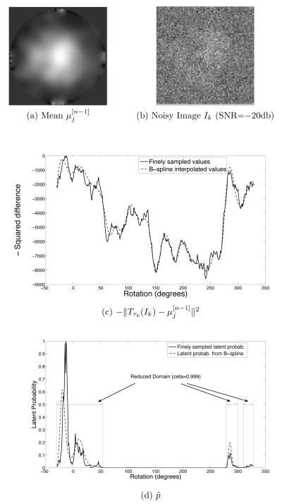
Both strategies are based on observations which are illustrated in figure 2. The (a) part of the figure shows an image which was obtained by projecting a ribosome structure in two different directions, summing the projections, adding noise, and blurring. This image is similar to an estimated class mean ${\mu }_j^{[n-1]}$ in the early iterations. The (b) part shows a single projection with white noise added to it. This image is similar to the observed images. The (c) part shows ${\Vert T_{-{\tau }_k}\left(I_k\right)-{\mu }_j^{[n-1]}\Vert }^2$ as a function of rotation (translations are held fixed for simplicity) with the image in part (a) as ${\mu }_j^{[n-1]}$ and the image in part (b) as I_k. The (d) part shows how $\tilde{p}$, which is calculated from ${\Vert T_{-{\tau }_k}\left(I_k\right)-{\mu }_j^{[n-1]}\Vert }^2$, behaves with rotation. The function $\tilde{p}$ has strong spikes.

Figure 2.

Domain Reduction and Grid Interpolation.

Figure 2 illustrates several effects:

1. The function $\tilde{p}$ has more than one peak. A peak-seeking alignment method would align I_k at the strongest of these peaks. But it is not clear that just using the strongest peak is the best alignment decision, especially since it is the best alignment to an unconverged mean ${\mu }_j^{[n-1]}$.

   On the other hand, recall from equations (9-10) that the EM algorithm works by using all values of $\tilde{p}$. Thus, all peaks contribute in the EM algorithm, and it avoids the premature decision of using a single peak. This shows why the EM algorithm is preferable to a peak-seeking alignment algorithm.

2. In spite of multiple peaks, figure 2d suggests that $\tilde{p}$ is essentially zero over a significant part of Ω_jk. If the numerical integration can be restricted to only that part of the domain where $\tilde{p}$ contributes significantly, then considerable computational gain can be made without losing too much accuracy. This is the motivation behind domain reduction.

3. Note that ${\Vert T_{-{\tau }_k}\left(I_k\right)-{\mu }_j^{[n-1]}\Vert }^2$ is a much smoother function than $\tilde{p}$, which is a spiky function. This suggests a way to estimate the reduced domains: introduce a coarse grid in the domains Ω_kj, calculate ${\Vert T_{-{\tau }_k}\left(I_k\right)-{\mu }_j^{[n-1]}\Vert }^2$ at the vertices of the coarse grid, interpolate using the vertex values and use interpolated function to estimate $\tilde{p}$ and the reduced domains. This is grid interpolation.

   The solid line in figure 2 c shows ${\Vert T_{-{\tau }_k}\left(I_k\right)-{\mu }_j^{[n-1]}\Vert }^2$ evaluated on a fine grid (spacing 1 degree). The dashed line in figure 2 c shows ${\Vert T_{-{\tau }_k}\left(I_k\right)-{\mu }_j^{[n-1]}\Vert }^2$ evaluated on a coarse grid (spacing 12 degrees) and interpolated by a B-spline. The resulting $\tilde{p}$’s are shown in figure 2 d. Note that the $\tilde{p}$ calculated from the B-spline gives an approximation of $\tilde{p}$ and the figure suggests that the reduced domain can be calculated from this approximation.

   The procedure that obtains the reduced domain is described below in detail. The result of using that procedure gives the reduced domain shown in figure 2 d (the parameter ζ is explained below).

We now describe both strategies in detail:

3.2 Domain Reduction

The idea in domain reduction is to replace integration over Ω_jk with integration over a smaller subset ${\Omega }_{jk}^{\ast }$. The ${\Omega }_{jk}^{\ast }$s are estimated to contain a significant fraction ζ of the probability mass of $\tilde{p}$. The fraction of the probability mass is equal to a parameter ζ is user-chosen but constrained to be 0 < ζ < 1. Because we want to retain the averaging properties of the EM-algorithm, we set the value of ζ close to 1, e.g. ζ = 0.999. Even though the ζ is very close to 1, the domain is reduced considerably because $\tilde{p}$ is spiky.

To describe more precisely how ${\Omega }_{jk}^{\ast }$ are found, recall that $\tilde{p}$ is obtained by column and row normalization as shown in figure 1. Thus the integral of $\tilde{p}$ sums to 1 in each row of ʊ. Let Ω_j = ∪_kΩ_jk be the union of all Ω_jk in a row, then row normalization implies that ${\int }_{{\Omega }_j}\tilde{p}d\tau =1$. Let O ⊂ Ω_j be any subset of Ω_j, then

$${\int }_O\tilde{p}d\tau$$

measures the probability “mass” of $\tilde{p}$ in O. Let O* be the subset of Ω_j with the smallest volume that has a probability mass of ζ:

$$O^{\ast }=\arg \underset{O}{\min }\mathrm{vol}\left(O\right)\text{subject to the constraints}O\subset {\Omega }_j,\text{and}{\int }_O\tilde{p}d\tau =\zeta .$$ (11)

Then, the reduced domain is ${\Omega }_{jk}^{\ast }=O^{\ast }\cap {\Omega }_{jk}$.

The reduced domain O* is easy to find: Let Τ be a threshold and ${\Omega }_j^{\tau }$ be the subset of Ω_j in which the values of $\tilde{p}$ are greater than or equal to Τ. Then ${\int }_{{\Omega }_j^{\tau }}\tilde{p}d\tau$ is a monotonically decreasing function of Τ and its range of values is [0, 1]. Thus there is a unique Τ for which ${\int }_{{\Omega }_j^{\tau }}\tilde{p}d\tau =\zeta$. It is straight forward to show that for this Τ the set ${\Omega }_j^{\tau }\tau$ equals the set O* of equation (11).

The algorithm for domain reduction is a binary-search algorithm for the appropriate Τ is :

The Domain Reduction Algorithm

1. Initialize: Set the upper and lower limit of Τ to 0 and 1 respectively.

2. Binary search: Carry out a binary search in within [0, 1] for the Τ that solves:

   $${\int }_{{\Omega }_j^{\tau }}\tilde{p}d\tau =\zeta .$$

3. Calculate the domains: Return the reduced domains ${\Omega }_{jk}^{\ast }={\Omega }_j^{\tau }\cap {\Omega }_{jk}$.

3.3 Grid Interpolation

Grid interpolation uses two grids, a coarse grid G_c and a fine grid G_f . The two grids are chosen such that any cube of the coarse grid contains an integer number of the cubes of the fine grid. The two grids are used to estimate the reduced domain as follows:

Domain Reduction with Grid Interpolation

1. Coarse Calculation: Calculate ${\Vert T_{-{\tau }_k}\left(I_k\right)-{\mu }_j^{[n-1]}\Vert }^2$ at the vertices of the coarse grid G_c.

2. Interpolate: Use a tensor product B-spline to interpolate the above values on to the fine grid G_f . B-spline interpolation is much faster than calculating ${\Vert T_{-{\tau }_k}\left(I_k\right)-{\mu }_j^{[n-1]}\Vert }^2$ at every node.

3. Estimate $\tilde{p}$: Use the interpolated values of ${\Vert T_{-{\tau }_k}\left(I_k\right)-{\mu }_j^{[n-1]}\Vert }^2$ to calculate $\tilde{p}$ using equations (6-7). Integrals are evaluated by Riemann sums over all vertices of the grid G_f .

4. Estimate reduced domain: For each row of ʊ, use binary search to find a threshold Τ such that the Riemann sum (integral) over all vertices of G_f for which $\tilde{p}\ge \tau$ is ζ. In the k^th row, let V = {v} denote all vertices in G_f for which $\tilde{p}\ge \tau$. Set $O_j^{\ast }={\cup }_{v\in V}C\left(v\right)$ where C(v) is the cube associated with vertex v, and the reduced domain to ${\Omega }_{jk}^{\ast }=O_j^{\ast }\cap {\Omega }_{jk}$.

3.4 Adaptive-EM

The adaptive-EM algorithm uses domain reduction with grid interpolation as an intermediate step in the calculations.

The Adaptive-EM Algorithm

1. Initialize: Set n = 0 and initialize ${\alpha }_j^{\left[0\right]}$, ${\mu }_j^{\left[0\right]}$, σ^[0] for j = 1, … ,M.

2. Start Iteration: Set n = n + 1.

3. Domain Reduction: For each row of ʊ use the domain reduction with grid interpolation to get the reduced domains ${\Omega }_{jk}^{\ast }$.

4. Calculate Latent Probabilities: For every vertex of the fine grid G_f , (re-)calculate the latent probabilities using equations (6-7). All integrals in these equations are calculated by a Riemann sum only over those vertices of the fine grid that lie in the reduced domains ${\Omega }_{jk}^{\ast }$.

5. Update Parameters: Update parameters ${\alpha }_j^{\left[n\right]}$, ${\mu }_j^{\left[n\right]}$, σ^[n] according to equations (8-10). Again all integrals in these equations are approximated by a Riemann sum over the vertices of the fine grid that lie in the reduced domains ${\Omega }_{jk}^{\ast }$.

6. Loop: Stop if ${\alpha }_j^{\left[n\right]}$, ${\mu }_j^{\left[n\right]}$, σ^[n] have converged. Else go to step 2.

Thus, the adaptive-EM algorithm is just the EM algorithm with the integrals replaced by Riemann sums over the vertices of the fine grid in the reduced domain.

4 Computational Complexity

The execution times of the EM and the adaptive-EM algorithm depend on factors that are implementation and machine dependent. For example, in a MATLAB implementation of the algorithm the computationally most expensive step is the calculation of the transformed image T_τk (I_k) at every vertex of the grid. On the other hand, in a CUDA implementation using graphics processors (GPUs, described in section 5), the image transformation is very fast and the computational speed is limited additionally by the norm calculation ${\Vert T_{-{\tau }_k}\left(I_k\right)-{\mu }_j^{[n-1]}\Vert }^2$. Furthermore, the actual execution time depends on the number of parallel GPU units available. All of these factors are implementation dependent.

However, the number of image transformations and the number of norm calculations are directly proportional to the number of vertices at which various integrands are evaluated. The number vertices processed per iteration depends only on the grid size and (for the adaptive-EM algorithm) the reduced domain. It is a relatively implementation independent performance measure. We use the ratio of the number of vertices processed per iteration for the EM algorithm to the number of vertices processed per iteration for the adaptive-EM algorithm as a measure of the speed up of the adaptive-EM algorithm.

Suppose that coarse and the fine grid have N_c and N_f vertices respectively in each domain Ω_kj and that the standard EM algorithm uses the fine grid while the adaptive EM algorithm uses the coarse and the fine grid.

The standard EM algorithm uses all vertices of the fine grid twice - once during the calculation in equation (6) and once during the parameter update in equations (9) and (10). Thus the total number of vertices per iteration is 2NMN_f , where N is the number of images and M is the number of class means.

The adaptive-EM algorithm uses vertices thrice - vertices of the coarse grid are used once in the domain reduction algorithm, and vertices of the fine grid in the reduced domain are used once in calculating latent probability and again in parameter update. Assuming that ρ percent of the vertices of the fine grid survive the domain reduction step, the net number of image transformations for calculating the latent probability plus the parameter update is 2NMρN_f . Thus, the net number of transformations is NMN_c + 2NMρN_f and the speedup factor s of the adaptive-EM algorithm is

$$s=\frac{2NM{N}_f}{NM{N}_c+2NM\rho N_f}=\frac{2\frac{N_f}{N_c}}{1+2\rho \frac{N_f}{N_c}}.$$ (12)

5 GPGPU programming

Modern off-the-shelf graphics cards for desktop computers have graphics processors with multiple processing units. These processors are capable of massive parallelism and are increasingly used for general purpose computing. We implemented the EM and adaptive-EM algorithms for parallel execution on NVIDIA graphics cards. We now briefly explain the programming environment and hardware model, and then describe our implementation of the algorithms.

The NVIDIA graphics architecture consists of an array of multiprocessors, each multiprocessor containing eight scalar processors, special function units, a multithread instruction unit, and local shared memory. The NVIDIA graphics processors are programmed by an extension of the C programming language called CUDA[7]. CUDA provides extended C functions (subroutines) called kernels. Multiple copies of a single kernel can be executed in parallel on graphics processors.

A part of the graphics memory can be configured as texture memory. When a two dimensional matrix, such as an image, is stored in texture memory, hardware support (fast interpolation) is available for addressing the matrix with real valued indices, i.e., if I is a N × N matrix stored in texture memory, then I can be indexed by a pair of real valued indices (x, y) ∈ [0, 1]×[0, 1]. The value at (x, y) is taken to be the interpolated value of I(x * (N − 1) + 1, y * (N − 1) + 1). The interpolation is linear and uses integer neighbors of this location. For the EM and adaptive-EM algorithms, the interpolation allows fast calculation of T_τ (I). Given, the transformation parameter τ = (θ, t_x, t_y), the transformed image T_−τ (I) is obtained by calculating T_−τ (I)(x, y) = I(x’, y’) where

$$\left[\begin{array}{c}\hfill x^{\prime }\hfill \\ \hfill y^{\prime }\hfill \end{array}\right]=\left[\begin{array}{cc}\hfill \cos \theta \hfill & \hfill \sin \theta \hfill \\ \hfill -\sin \theta \hfill & \hfill \cos \theta \hfill \end{array}\right]\left[\begin{array}{c}\hfill x-1∕2\hfill \\ \hfill y-1∕2\hfill \end{array}\right]-\left[\begin{array}{c}\hfill 1∕2\hfill \\ \hfill 1∕2\hfill \end{array}\right]\left[\begin{array}{c}\hfill t_x∕(N∕2)\hfill \\ \hfill t_y∕(N∕2)\hfill \end{array}\right],$$

and x, y is sampled on an N ×N grid in [0, 1]×[0, 1]. Furthermore, in the CUDA model, texture memory is persistent so that an image need be loaded only once into texture memory before the transformation is calculated for different values of τ .

A CUDA program runs on the host CPU as well as the graphics processors. Typically, only a small part of any algorithm is computationally expensive, and that part is parallelized as a kernel and executed on the graphics processors. The rest of the algorithm is executed on the host CPU serially. For further details of hardware, thread and block scheduling, and texture memory the reader is referred to the CUDA programming manual [4, 7].

5.1 CUDA implementation of the EM and adaptive-EM algorithm

There are two computationally expensive parts of the EM and adaptive-EM algorithm: the calculation of latent probabilities of equations (6-7) and the Riemann sums for the parameter updates needed for equations (9-10). Our CUDA implementation uses three kernels for these two tasks.

All of our kernels iterate over a set of transformations {τ}. The elements of this set depend on whether the kernel is used for the EM algorithm or the adaptive-EM algorithm. All kernels are run by first loading the set of transformations {τ}. The kernels are as follows:

• Kernel 1 (Transformation Kernel): This kernel calculates T_−τk (I_k). Before the kernel is executed the set of transformations {τ} is loaded into the graphics memory. Then, texture memory is allocated and I_k is loaded into it. The kernel rotates and translates I_k according to values of τ_k ∈ {τ} stored in the memory.

  Even faster methods for computing the integrals can be envisioned, based on the polar FFT approach of Penczek [14].

• Kernel 2 (Norm Kernel): Given T_−τk (I_k) and ${\mu }_j^{[n-1]}$ this kernel calculates ${\Vert T_{-{\tau }_k}\left(I_k\right)-{\mu }_j^{[n-1]}\Vert }^2$.

• Kernel 3 (Parameter Calculation Kernel): For every j = 1, … ,M the sum over k in equation (9) and the inner sum over k and the Riemann integral in the summand in equation (10) is carried out in parallel by this kernel.

6 Simulations

The EM and adaptive-EM algorithms were evaluated using simulations. The 3D ribosome structure of figure 3a was used in the simulations. The structure has a resolution of 2.82Å per side of a voxel. The structure was projected along the x-, y-, and z-axis to obtain the images shown in figures 3 b,c,d. All projections were 128 pixels × 128 pixels. The electron-microscope contrast transfer function (CTF) [3] of the form:

$$\mathit{ct}f\left(w\right)=a+(1-a)\sin \left(\alpha {\Vert \omega \Vert }^2\right),$$

was applied to the projections with a = 0.07 and α set to a value such that the first zero of the CTF occurred at 1.6nm.

Figure 3.

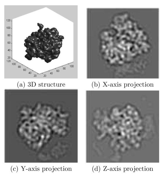
Ribosome structure and projections.

Each projection was randomly rotated between 0 and 360 degrees, randomly translated by ±2 pixels in the x- and y-directions, and contaminated with additive white noise to create one image. A total of 900 such images were created from the three projections (300 images per projection). Preliminary experimentation showed that, for 900 images, the EM algorithm failed at a signal-to-noise ratio (SNR) of −22db. We chose SNRs of −15db and −21db for simulations. These SNRs represent images at low and high noise respectively.

The CUDA implementation of the EM and adaptive-EM algorithms was used in the simulations. All simulations were carried out on a single desktop computer. All algorithms were initialized with class means set to random zero-mean noise.

Performance measures

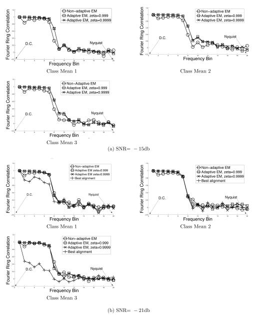
Because the adaptive algorithm uses a reduced domain, its estimates of the class means are different than those of the EM algorithm. The adaptive strategy is useful if this difference is small. To evaluate the difference, we compared the class means of the EM algorithm and the adaptive-EM algorithm with the non-noisy projections (which provide “ground truth”) using Fourier ring correlations. The Fourier ring correlations were measured by partitioning the Fourier space into 20 equally spaced radial shells from dc to the Nyquist frequency and calculating the correlation coefficient in each ring.

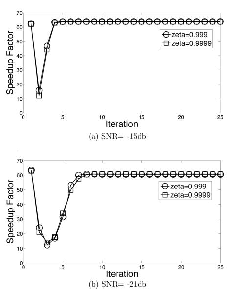
A second measure for comparing the adaptive-EM with EM is computational complexity. As discussed above, we do this by measuring the ratio of the number of vertices processed per iteration of the EM algorithm to the number of vertices processed per iteration of the adaptive-EM algorithm. This is the speedup factor s of equation (12) measured every iteration.

Algorithm Parameters

In all simulations the domain Ω was set to [0°, 360°]×[−2pix, 2pix]×[−2pix, 2pix]. The fine grid sampled this volume at a resolution of Δθ = 1°, and Δt_x =Δt_y = 1 pixels. The coarse grid resolution was Δθ = 12°, and Δt_x = Δt_y = 2 pixels.

Preliminary informal experimentation revealed that the adaptive-EM algorithm gave reasonable class means for ζ = 0.999 and 0.9999. These values were used for further investigation.

In all simulations, both algorithms converged by the 25th iteration.

6.1 EM and Adaptive-EM Algorithms

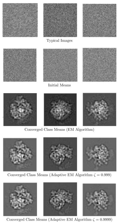
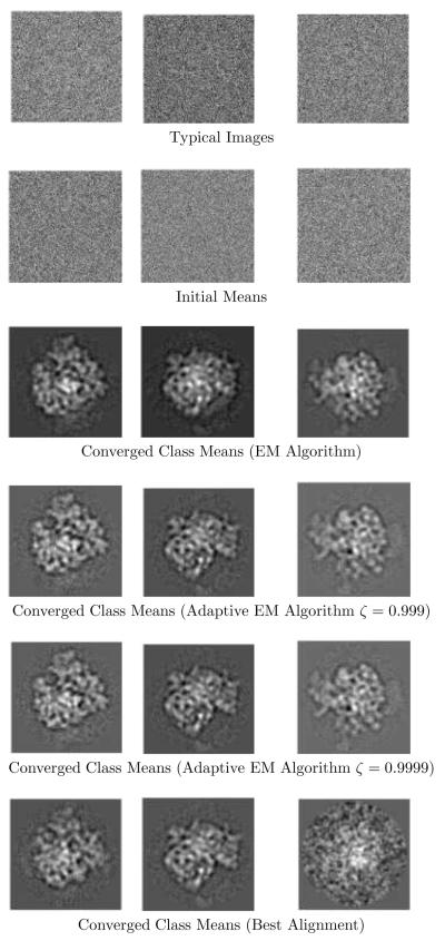
Figures 4-5 shows the results of using the EM algorithm and the adaptive-EM algorithm for image pixel S.N.R.’s of −15db and −21db respectively.

Figure 4.

EM and adaptive-EM reconstructions at SNR= −15db.

Figure 5.

EM and adaptive-EM reconstructions at SNR= −22db.

The top rows in both figures show sample noisy images from x-,y-, and z-axis projections. The next row shows the class means used to initialize the algorithms. Subsequent rows show the class means obtained by the EM algorithm, and by the adaptive-EM algorithm for ζ = 0.999 and ζ = 0.9999. For SNR=−21db, we also obtained the “best alignment” class means in order to compare them with the EM class means. These are shown in the bottom row of figure 5.

Figure 6 a-c shows the Fourier ring correlations between the class means and the corresponding “ground truth” class means of figure 3b-d.

Figure 6.

Fourier ring correlations of EM and adaptive-EM class means compared to ground truth.

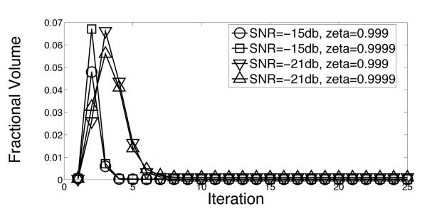
The speedup factors s (eq. (12)) of the adaptive-EM algorithm are shown as a function of iteration number in figure 7. At termination, the speedup factors are above 60.0 for SNR = −15 and −21db. Note that the speedup factors for all iterations, including the first iteration, is greater than 10. Recall from equation (12) that the speed up factor depends on ρ, which is the fraction of vertices surviving in the reduced domain. Using equation (12) to solve for ρ gives figure 8 for the data of figure 7.

Figure 7.

Speedup of the adaptive-EM algorithm.

Figure 8.

Ratio of number of vertices of the reduced domain to the number of vertices in Ω.

A final comment. Although the main goal of the simulations was to measure the speed-up of the adaptive-EM algorithm over the EM algorithm, we also attempted to measure and compare the execution speed of the GPGPU algorithm with the execution speed of a MATLAB implementation. Unfortunately, the MATLAB implementation was not fast enough to process 900 images in over 10 days. An informal comparison of speed with smaller number of images, and higher SNR (SNR=−15db) revealed that the GPGPU implementation was faster by factor of 80 or more than the MATLAB implementation.

6.2 Discussion

The data in figures 4-6 suggests that domain reduction and grid interpolation are effective strategies for reducing computation in the EM algorithm. A curious feature of adaptive-EM algorithm is that its Fourier ring correlations are marginally better than those of the EM algorithm. This can be attributed to the the fact that contributions from the reduced domain are better matched to the class mean (alternately, contributions from outside the reduced domain are ill-matched to the class mean). Nevertheless, the effective resolutions of the EM algorithm and the adaptive-EM algorithm are the practically identical, showing that there is little penalty for using the reduced domain.

The last row of figure 5 shows dramatically the failure of the “best alignment” strategy for noisy images. Notice especially the poor reconstruction of the last class mean. The EM algorithm, on the other hand, accurately recovered all three means, as did the adaptive EM algorithm in this challenging case with a very low SNR.

The data in figures 7-8 shows that the adaptive strategy is effective in reducing computation. The average speedups for all SNRs that we measured are above 10, suggesting that CPU-months worth of computation may be reduced to CPU-days worth of computation. Two other points are also worth noting. First, the adaptive strategy is very effective even in the first iteration. This is significantly different from the stategy of Scheres et. al. [9] where the first iteration is carried without any speedup. Second, figure 8 shows the part of the domain which contributes effectively to the calculation stabilizes after a variable number of iterations. For SNR= −21db, for example, the domain does not appear to stabilize till the 10th iteration. This suggests that a strategy which prematurely freezes the reduced domain, or which does not estimate the significance of all rotations and translations before adaptation, may not be optimal.

In the simulations shown here the coarse grid had the particularly large angular step of 12°. This had the advantage of a low number of vertices to be evaluated, but the disadvantage that the interpolated function deviated substantially from the true values on the fine grid, as shown in Figure 2. This in turn required that the parameter ζ be set to a conservative value (e.g. 0.999) to ensure that the reduced domain encompassed all of the important contributions to the latent probability. A smaller coarse-grid step would have the advantage that the interpolated function better approximates the true values, and in this case the value of the ζ parameter would more accurately reflect the fraction of the integrand that is preserved. In the end it is not only the coarse-grid step size, but also the fraction of fine-grid nodes that survive the domain reduction, that determine the speed-up of the algorithm (eqn. 12).

7 Conclusion

The EM algorithm for cryo-EM is computationally expensive because the E step requires numerical integration. However, the latent data probabilities for cryo-EM tend to be spiky and the computational complexity of the EM algorithm can be reduced by limiting the numerical integration to a reduced domain which contains most of the probability mass of the latent data. Furthermore, the reduced domain can be effectively estimated by a grid interpolation strategy. Using the reduced domain and grid interpolation gives an adaptive-EM algorithm. This algorithm adjusts its integration domain in each iteration. Simulations show that the adaptive-EM algorithm provides speedup of over a factor of 10 even in the first iteration. The speedup at termination is greater than a factor of 60. Simulations also show that the adaptive-EM algorithm gives class means that are practically identical to the EM class means.

References

- [1].Atkinson KE. An Introduction to Numerical Analysis. John Wiley and Sons; 1978. [Google Scholar]
- [2].Castano-Diez D, Moser D, Schoenegger A, Pruggnaller S, Frangakis AS. Performance evaluation of image processing algorithms on the GPU. J Struct Biol. 2008;164:153–60. doi: 10.1016/j.jsb.2008.07.006. [DOI] [PubMed] [Google Scholar]
- [3].Frank J. Three-dimensional Electron Microscopy of Macromolecular Assemblies. Oxford University Press; 2006. [Google Scholar]
- [4].Kirk D, Hwu WW. Programming Massively Parallel Processors. Morgan Kaufmann Publishers; 2010. [Google Scholar]
- [5].Lee J, Doerschuk PC, Johnson JE. Exact reduced-complexity maximum likelihood re-construction of multiple 3-D objects from unlabeled unoriented 2-D projections and electron microscopy of viruses. IEEE Trans Image Process. 2007;16:2865–78. doi: 10.1109/tip.2007.908298. [DOI] [PubMed] [Google Scholar]
- [6].McLachlan G, Peel D. Finite Mixture Models. Wiley-Interscience; 2000. [Google Scholar]
- [7].NVIDIA CUDA Compute Unified Device Architecture . Programming Guide. Version 2.0 nVIDIA Corporation; 2007-2008. [Google Scholar]
- [8].Sander B, Golas MM, Stark H. Corrim-based alignment for improved speed in single-particle image processing. J Struct Biol. 2003;143:219–28. doi: 10.1016/j.jsb.2003.08.001. [DOI] [PubMed] [Google Scholar]
- [9].Scheres SHW, Valle M, Carazo J-M. Fast Maximum-likelihood Refinement of Electron Microscopy Images. Bioinformatics. 2005;vol. 21(Suppl. 2):243–244. doi: 10.1093/bioinformatics/bti1140. [DOI] [PubMed] [Google Scholar]
- [10].Scheres SH, Nunez-Ramirez R, Gomez-Llorente Y, San Martin C, Eggermont PP, Carazo JM. Modeling experimental image formation for likelihood-based classification of electron microscopy data. Structure. 2007a;15:1167–77. doi: 10.1016/j.str.2007.09.003. [DOI] [PMC free article] [PubMed] [Google Scholar]
- [11].Scheres SH, Valle M, Nunez R, Sorzano CO, Marabini R, Herman GT, Carazo JM. Maximum-likelihood multi-reference refinement for electron microscopy images. J Mol Biol. 2005b;348:139–49. doi: 10.1016/j.jmb.2005.02.031. [DOI] [PubMed] [Google Scholar]
- [12].Scheres SH, Gao H, Valle M, Herman GT, Eggermont PP, Frank J, Carazo JM. Disentangling conformational states of macromolecules in 3D-EM through likelihood optimization. Nat Methods. 2007b;4:27–9. doi: 10.1038/nmeth992. [DOI] [PubMed] [Google Scholar]
- [13].Sigworth FJ. A maximum-likelihood approach to single-particle image refinement. J Struct Biol. 1998;122:328–39. doi: 10.1006/jsbi.1998.4014. [DOI] [PubMed] [Google Scholar]
- [14].Yang Z, Penczek Cryo-EM image alignment based on nonuniform fast Fourier Transform. Ultra-microscopy. 2008;108:959–969. doi: 10.1016/j.ultramic.2008.03.006. [DOI] [PMC free article] [PubMed] [Google Scholar]
- [15].Yin Z, Zheng Y, Doerschuk PC. An ab initio algorithm for low-resolution 3-D reconstructions from cryoelectron microscopy images. J Struct Biol. 2001;133:132–42. doi: 10.1006/jsbi.2001.4356. [DOI] [PubMed] [Google Scholar]
- [16].Yin Z, Zheng Y, Doerschuk PC, Natarajan P, Johnson JE. A statistical approach to computer processing of cryo-electron microscope images: virion classification and 3-D reconstruction. J Struct Biol. 2003;144:24–50. doi: 10.1016/j.jsb.2003.09.023. [DOI] [PubMed] [Google Scholar]
- [17].Zeng X, Stahlberg H, Grigorieff N. A maximum likelihood approach to two-dimensional crystals. J Struct Biol. 2007;160:362–74. doi: 10.1016/j.jsb.2007.09.013. [DOI] [PMC free article] [PubMed] [Google Scholar]