Methods for building an inexpensive computer-controlled olfactometer for temporally precise experiments

Abstract

Many human olfactory experiments call for fast and stable stimulus-rise times as well as exact and stable stimulus-onset times. Due to these temporal demands, an olfactometer is often needed. However, an olfactometer is a piece of equipment that either comes with a high price tag or requires a high degree of technical expertise to build and/or to run. Here, we detail the construction of an olfactometer that is constructed almost exclusively with “off-the-shelf” parts, requires little technical knowledge to build, has relatively low price tags, and is controlled by E-Prime, a turnkey-ready and easily-programmable software commonly used in psychological experiments. The olfactometer can present either solid or liquid odor sources, and it exhibits a fast stimulus-rise time and a fast and stable stimulus-onset time. We provide a detailed description of the olfactometer construction, a list of its individual parts and prices, as well as potential modifications to the design. In addition, we present odor onset and concentration curves as measured with a photoionization detector, together with corresponding GC/MS analyses of signal-intensity drop (5.9%) over a longer period of use. Finally, we present data from behavioral and psychophysiological recordings demonstrating that the olfactometer is suitable for use during event-related EEG experiments.

1. Introduction

Researchers of perception, independent of sensory modality, must have precise control of their stimuli. However, researchers studying the chemical senses face a unique problem: olfactory and gustatory stimuli are short-lived and difficult to present with inexpensive and commercially-available equipment. Whereas students of the visual and auditory senses are able to present stimuli repeatedly in a highly precise manner, both spatially and temporally, students of olfaction are faced with the challenge of delivering finite structural objects (molecules) whose percept changes over time.

The most common solution, and often the most inexpensive and preferable solution, is to present odors in bottles of various kinds. However, when any form of temporal control is needed, whether for measures of reaction time or event-related psychophysiological measures such as skin conductance response, an olfactometer is necessary. The few olfactometers that are currently commercially-available as a turnkey solution are expensive, and they often exceed either a researcher’s financial limits or the technical reach of a researcher whose lab is not dedicated solely to olfactory research. This often leaves the researcher with no other option than to build his or her own olfactometer. Several olfactometers meant to be used with both human and non-human animals have been described in the literature (Benignus & Prah, 1980; deWijk, Vaessen, Heidema, & Koster, 1996; Etcheto, 1980; Johnson & Sobel, 2007; Kobal, 1985; Lorig, Elmes, Zald, & Pardo, 1999; Lowen & Lukas, 2006; Morton, Castro, & Eichenbaum, 1982; Owen, Patterson, & Simpson, 2002; Saito, Iida, Sakaguchi, & Kodama, 1984; Slotnick & Nigrosh, 1974; Vigouroux, Viret, & Duchamp, 1988). However, most of these olfactometers demand a considerable amount of skilled labor for the construction of essential parts, knowledge about electronics and fluid mechanics for wiring and air connections, and programming knowledge to create the control program. Moreover, even if one were able to construct one of the aforementioned olfactometers, most allow for the use of only a limited number of odors (odor channels), often in the range of one to six odors. In short, the individual neuroscientist faces often insurmountable financial barriers in the acquisition of a commercially-available olfactometer and equally overwhelming skill, knowledge, and time requirements for the construction of an olfactometer. These obstacles necessitate a more primitive presentation of the odor stimulus, which is unsuitable for experimental designs demanding precise temporal control. With this manuscript, we aim to provide the neuroscience community with a detailed description of a computer-controlled olfactometer that requires no special talent to assemble or operate, yet is suitable for most behavioral and EEG studies with olfactory stimuli.

Stable and controlled stimulus presentation is required for good signal measurement. Delivered odor stimuli must display several characteristics, such as a square-shaped form (steep rise time; stable concentration; steep offset), a fast and consistent onset enabling synchronous delivery with other presented stimuli, and a presentation void of tactile cues (such as a change in airflow). The challenges described above have been met in various ways in previously-described olfactometer designs. For an olfactometer with good temporal control, two general design categories can be identified in the literature: continuous flow olfactometers (Kobal, 1985) and so-called “Lorig design” olfactometers (Lorig et al., 1999). Both designs offer unique advantages and problems.

Continuous flow olfactometers enable very fast onset and offset timing, thereby creating a nice, square-shaped stimulus presentation. In these designs, air flows continuously through or over the odor source and is then transported via tubing to the subject. Vacuum pressure plays an important role in a continuous flow olfactometer, where it is utilized both to switch between odorized air flow and control flow and to evacuate odors, often just below the subject’s nose. The vacuum pressure that controls the stimulus onset and offset, however, must be carefully calibrated using expensive mass flow control meters. Too much vacuum pressure will suck back all odors, and too little vacuum pressure will allow for contamination by residual odors. Moreover, this design is most commonly used to present odors in liquid form. In brief, continuous flow olfactometers provide optimal stimulus control, but the necessity of using mass flow control meters and two separate air systems (pressure and vacuum) add significant expense and complexity, complexity associated primarily with programming control software.

The so-called “Lorig design” (Lorig et al., 1999) is based on a simple principle that the odor sources are contained in small reservoirs near the subject, and the individual solenoid valves that effectively turn the odors on and off by opening and closing air access to each odor channel are located at a distance from the odor source. In addition, the flow through each odor channel is independently regulated by an individual flowmeter. Due to the simpler design, few individual parts, and minimal labor requirements, this design has the benefit of a reduced total cost relative to other designs mentioned in the literature. However, due to the distance between the valves and odor reservoir, and due to the low airflow that results in a slow perfusion of air through tubing leading to the subject’s nose, the exact time of odor onset is hard to determine accurately.

The olfactometer described here resolves the complexity issues and timing issues for these two most common olfactometer designs by utilizing newly-developed check valves and by controlling the solenoid valves via commercially-available valve control units, which – in turn – can be triggered by all of the most commonly used stimulus presentation/response recording programs such as E-Prime, Presentation, SuperLab, PowerLab, etc. This olfactometer presents stable concentrations of volatile compounds to the subject with precise delivery onset and offset, and it eliminates any need for vacuum to achieve the steep rise times mandated by event-related stimulation designs.

When we set out to construct this olfactometer, we had the following major goals: First, all parts should be “off-the-shelf” and require minimal customization. Second, required regular maintenance should be minimal, and changing odorants between experiments should involve the replacement/cleaning of as few parts as possible. Third, the olfactometer should be controlled by an “off-the-shelf” control software program with no required customization. Fourth, the financial and time costs associated with building the olfactometer should be minimal and should allow for easy modification of the design. Fifth, the olfactometer should be capable of delivering a large number of odorants. Sixth, the olfactometer should present odors with a stable onset time and concentration, as well as a rise time fast enough to be suitable for event-related stimulation designs. Seventh, the olfactometer should be compatible with liquid, solid, and gaseous odor sources, including odor pads (commonly used to present body odors) and sources of “real odor” (mashed banana, sliced apple, etc.). Eighth, the olfactometer should be transportable and compact enough to store easily in the minimal space available in most academic settings.

We describe, in detail, an olfactometer suitable for behavioral experiments demanding a level of precise temporal control near, or at, the temporal precision of visual stimuli. It is our hope that the description is specific enough to be used as a template, à la an IKEA manual. Some details of the olfactometer require manual construction beyond screwing two parts together. These items are identified in the enclosed Table 1, and suggested off-the-shelf replacements are suggested. However, we argue that an adult with enough technical knowledge to put up a shelf using both screws and plugs is capable of building the olfactometer described here. In addition to technical descriptions, we provide data describing the temporal performance of the olfactometer, and we detail the expected stimulus-concentration drop during a normal experimental session by means of Gas Chromatography/Mass Spectroscopy (GC/MS). Finally, proof of principle is provided via recordings of evoked skin conductance responses (SCR) and cortical chemosensory event-related potentials (ERP) derived from an ongoing EEG recording.

Identifying #	Item	Item#	Vendor / Manufacturer	Price (USD)	Qt	Summed Price
	Olfactometer cabinet	LUNDSTROM-BHV-3	Rankin Automation	$1,000	1	$1,000
1	Air compressor	2685PE40 (MFR#)	Ralph A. Hiller	$496	1	$496
2	Laboratory Gas Drying Unit	26840	Hammond Drierite	$79	1	$79
3	Pressure Regulator, Type 41	68825-26	Cole-Parmer	$62	1	$62
4	Flowmeter System, Direct-reading Flowtube (5.0 L/m)	32047-13	Cole-Parmer	$42	8	$336
4	Multitube Flowmeter System, Multitibe Frame (4 tube)	03214-50	Cole-Parmer	$209	1	$209
4	Flowmeter System, Multitibe Frame (5 tube)	03214-64	Cole-Parmer	$255	1	$255
4	Flowmeter System, Valve Cartridges	03217-92	Cole-Parmer	$40	9	$360
5	Nylon manifold (2-outlet)	31522-31	Cole-Parmer	$23	1	$23
6	Flowmeter System, Direct-reading Flowtube (1.15 L/m)	32047-10	Cole-Parmer	$42	1	$42
7	Monell Valve Manifold (3-way valves)	(SPECIALTY ITEM)	Automate Scientific	$1,000	1	$1,000
8	NPT Check Valves (Series 200) (on polycarbonate odorant reservoir)	214214PB-0007S000- 2959	Smart Products, Inc.	$5	16	$82
8	NPT Check Valves (Series 200) (on glass odorant reservoir)	204204PB-0011S000- 2959	Smart Products, Inc.	$5	16	$82
9	ODOR RESERVOIRS (PLEASE SEE BELOW)
10	LF3000® Multi-connector, Male screw body	3320-53-00-12	Rankin Automation	$94	1	$94
10	LF3000® Multi-connector, Female screw body	3321-53-00-12	Rankin Automation	$94	1	$94
10	LF3000® Multi-connector, Screw cap	3329-00-03	Rankin Automation	$28	1	$28
10	Through-wall Coupling, Push-to-Connect Tube Fitting	5779K675	McMaster-Carr	$4	1	$4
11	ValveLink 8.2 Digital/Manual Controller	01–18	AutoMate Scientific	$995	1	$995
Odor Reservoirs	Item	Item#	Vendor	Price/PK	Qt	Summed Price
3A	Small polycarbonate reservoir, liquid odorants	2116-0060 (MFR#)	Fisher Scientific	$23.00	2	$46
3B	Large polycarbonate reservoir, solid odorants	2116-0125 (MFR#)	Fisher Scientific	$40.07	2	$80
3C	Glass reservoir, liquid odorants	(SPECIALTY ITEM)
				Total Price:		$5,284

2. Material and methods

Specific parts are referenced by manufacturers’ product names rather than by more generic terms, and each part is listed with its specific item number. In addition, a list of all the key components and their estimated costs can be found in Table 1.

Please note that the price listed for each item is the cost at the time of purchase (October 2009) and is not guaranteed by the manufacturer. Moreover, please note that we do not specifically endorse the vendors listed in this manuscript. Although we have been satisfied with the purchased materials, other suppliers, unbeknownst to us, may provide both cheaper and better products; we recommend that those interested in replicating the construction of this olfactometer query local distributors for price comparisons. We merely provide the following information as a service to the reader should they wish to replicate our work.

2.1 Olfactometer construction

2.1.1 Cabinet

Portability and easy storage were essential requirements for the olfactometer design. With these factors in mind, we constructed the olfactometer cabinet from lightweight, durable T-slotted 80/20 aluminum profiles (Rankin Automation, #LUNDSTROM-BHV-3; http://www.rankinautomation.com). The cabinet is mounted on large, lockable, 360° caster wheels to ensure ease of transport, and its external dimensions facilitate easy storage (H64cm × W50cm × D50cm). The cabinet consists of three sub-compartments (Figure 1), with shelves and sides composed of 5mm thick clear polycarbonate. Polycarbonate was chosen for its light weight, transparency, compatibility with other materials, and low cost.

Figure 1.

Olfactometer cabinet, compartments, and major components. Letters and numbers are outlined within the text.

The individual components within the cabinet will be described in detail below. However, as an overview: compartment [A] houses the air-supply unit [A1] (not seen in picture), the air-filtration unit [A2], and the pressure regulator and master flowmeter [not seen here]; compartment [B] houses the solenoid valves [B1], the odor reservoirs [B2], and the individual flow regulators [B3]; compartment [C] houses the valve controller [C1], the electronic connections [C2], and the outgoing air connections [C3]. The system is controlled by a standard laptop [D] or desktop computer with a DB-25 LPT port (commonly known as parallel or printer port).

2.1.2 Tubing and tube fittings – General overview

Regular tubing changes are essential to keep any olfactometer in optimal operating condition. In this design, only two tubing types require occasional changing. Before entering the valves, air is routed through 1/8” ID (inner diameter) polyurethane tubing, which was chosen for its low price, excellent durability, and compatibility with barbed and push-to-connect fittings. Although barbed fittings are commonly used and less expensive, push-to-connect fittings are more convenient, especially for temporary connections. After exiting the odor reservoirs, the air is odorized, and the primary factor in tubing selection is then limiting the risk of contamination. To carry the odorized air from the odor reservoirs to the subject’s nose, we chose 1/16” ID fluoropolymer tubing (PTFE, PFA, FEP, also sold under the brand name Teflon) for its high chemical resistance and non-reactivity to carry the odorized air from the odor reservoirs to the subject’s nose. This more rigid tubing is compatible with both push-to-connect and compression fittings. Throughout the olfactometer, four types of tube fittings are in use: push-to-connect fittings, quick-disconnect fittings, compression fittings, and barbed fittings. PTFE thread sealer tape (Cole-Parmer, #08752-27) was used with all threaded connections to limit leakage, a primary concern with any olfactometer.

2.1.3 Air supply

A detailed schematic of the olfactometer is provided in Figure 2, and, for clarity, we recommend consulting Figure 2 while reading this section. Air to operate the olfactometer can be supplied by either one of two systems: an external, high-pressure air supply (central air system) or an air compressor. Currently, we operate our olfactometer with air diverted from the central air system, which enters the olfactometer via polyurethane tubing and a quick-disconnect fitting. This arrangement is simpler and quieter than the alternative air compressor [Item 1, Figure 2] but dependent on access to a central air supply. In a setting without central air supply access, the olfactometer requires an air compressor capable of delivering large quantities of air (30 L/m) at a mid-range pressure (around 30 PSI or 2 bar). For several reasons, we use WOB-L piston compressors in our olfactometers despite the fact that they generate a considerable amount of noise (40–50 dB). Piston compressors deliver large quantities of air at decent pressures, and they are relatively small in size, durable, low-maintenance, and affordable. We have used Thomas pumps with good success (Gardner Denver-Thomas, #2685PE40; http://www.gd-thomas.com). The air supplied by the air compressor [1] is fed through large bore tubing (½” ID) to a pressure regulator [3] (Cole-Parmer, Marsh Bellofram, #68825-26), which regulates system pressure upstream of the channel-specific flowmeters. The cause for a pressure regulator and flowmeter combination is twofold. First, the pressure regulator itself maintains a steady pressure in the system. Unchecked, the compressor would pump air into the system continuously, and pressure would build up at the channel-specific flowmeters [4] downstream. Pressure differentials would increase over time, creating instability in the system and changes in airflow rate. Second, the pressure regulator can be calibrated to deliver a minimally sufficient flow, as measured by the accompanying flowmeter, for the desired number of channels, and excess air delivered from the compressor is vented from the regulator’s built-in bleed valves.

Figure 2.

Schematic drawing of the olfactometer. Numbers are outlined within the text.

2.1.4 Air filtration

Most sources of air have some level of detectable odor. Even air supplied from the central air systems in hospitals and other medical facilities often contains odorous impurities. In a worst-case scenario, this purportedly odor-free air would render an experiment’s baseline recording useless. To avoid this problem, all air supplied to the olfactometer from either an external central air supply or an internal compressor is cleaned of residual odors. We opted to modify a commercially-available drying unit [2] (W. A. Hammond Drierite, #26840; http://www.drierite.com) for use as a drying and filtering unit by adding active carbon, a well-established air filtration choice. Off-the-shelf, the Laboratory Gas Drying Unit contains only Indicating Drierite, a color-changing desiccant. Because the unit is designed to dry larger amounts of air than used in this application, we exchanged half of the Indicating Drierite for active carbon. In this olfactometer, incoming air flows through the air filtration unit before any other component, which ensures that the olfactometer’s air supply is dry and free of contaminants. In our experience, air supplied by the central air systems in hospitals or research institutes contains more than a negligible amount of moisture; however, if an air source is completely free of moisture, residual contaminants are the only remaining concern, and a less expensive option becomes viable. In that case, we recommend using the Drying Tube for Air (W. A. Hammond Drierite, #26930) and replacing all Indicating Drierite with active carbon.

2.1.5 Flow regulation

The dry filtered air is lead to a two-outlet manifold [5] (Cole-Parmer, #31522-31), which divides air into two streams. Once separated, these two airstreams flow into two Multitube Flowmeter frames mounted side-by-side on the cabinet door (Cole-Parmer, #03214-50, #03214-64). Each frame is constructed with a common inlet and parallel outlets, and – together – the frames further split the two air streams into 9 independent channels. The flowmeter frames are loaded with eight 5.0 L/m direct-reading flowtubes [4] (Cole-Parmer, #32047-13) and one 1.15 L/m direct-reading flowtube [6] (Cole-Parmer, #32047-10), and airflow through all is regulated by individual valve cartridges (Cole-Parmer, #03217-92). The advantage of utilizing the Multitube Flowmeter System is two-fold. First, the ability to independently regulate the airflow through each odor channel gives the experimenter great flexibility; multiple independent flowtubes allow for the use of as many or as few channels as necessary (the others can be closed to reduce airflow demand) and the use of different flows during a single experiment without having to re-calibrate the system. Second, by using flowmeter frames and exchangeable flowtubes, the experimenter can optimize the design of his/her olfactometer by choosing flowtubes appropriate for the airflow desired in each channel and/or experiment. The eight 5.0 L/m flowtubes regulate the airflow through the eight odor channels [4], and the 1.15 L/m flowtube regulates the airflow through the continuous flow (CF) line [6]. This CF line bypasses the solenoid valves and is directly connected to the nosepiece (described below in detail).

Now divided into nine separate channels, the air is directed away from the individual flowmeters to the channel-specific three-way solenoid valves [7]. An olfactometer should be able to deliver odors without any auditory, visual, or tactile cues. Two important factors in achieving this goal are the relative speed and silence of valve actuation; the valves must have a fast actuating time, and, to prevent auditory cues, the valves should produce as little noise as possible when actuated. Often, an olfactometer is located in the same room as the subject to limit the distance of odorized air transportation. If the valves produce a discernable sound, the subjects learn quickly to associate the sound with odor delivery, and they may even learn to discriminate odors based solely on the sounds of individual valves. In our experience, most solenoid valves on the market demonstrate a decent actuating time, but many also produce a loud noise when actuated. We use miniature, manifold-mounted, three-way solenoid valves (AutoMate Scientific Inc., Berkeley, CA, USA; http://www.autom8.com), which have an activation lag-time ranging from 1.5 – 4.0 ms and produce a nearly inaudible click when actuated. Because the valves are mounted on the inside of the olfactometer (Figure 2) with rubber gaskets between the screws and polycarbonate panel to reduce vibrations, valve actuation is inaudible even to subjects sitting nearby. Though unorthodox, the use of three-way regulatory valves eliminates the effects of pressure changes in the system as a result of valve actuation because – in contrast to two-way valves – three-way valves only switch the direction of a continuous airflow. In systems using two-way valves, there is a buildup of air pressure behind a closed valve that is released upon actuation; this sudden release of pressure creates a sharp airflow increase that travels downstream and is felt by the subject as an air-puff. In this system of three-way valves, continuous airflow is directed either into the olfactometer’s main compartment or to the odor reservoir, and no shift in system pressure occurs when a valve is actuated. An added benefit of this design is the flushing action of air exhausted from unactuated three-way valves, which prevents the accumulation of residual odors and contamination of the olfactometer.

2.1.6 Odor reservoirs

When a three-way valve is actuated and air is diverted through, the air passes a check valve before entering the odor reservoir [9]. The purpose of the check valve [8, Figure 2; B1, Figure 3A] (Smart Products Inc, #214214PB, #204204PB; http://www.smartproducts.com) is to prevent odorized air from flowing back towards the solenoid valve and contaminating the system. The odor reservoir is the only olfactometer component that must be custom-made, and this is due to the fact that, to the best of our knowledge, there are no pre-fabricated reservoirs that can be incorporated directly into this design. We currently use three alternative odor reservoirs: one small polycarbonate reservoir for liquid odorants [Figure 3A] (Fisher Scientific, Nalgene, #2116-0060), one large polycarbonate reservoir for non-liquid odor sources (such as odor pads and food objects) [Figure 3B] (Fisher Scientific, Nalgene, #2116-0125), and one glass reservoir custom-designed for liquid odorants [Figure 3C]. The small and large polycarbonate reservoirs require the addition of a PTFE block to the underside of the reservoir lid, which creates enough solid material for use of threaded fittings. Two holes are then drilled and threaded for the following fittings: for incoming air, the external aforementioned check valve [8] and an internal barbed fitting; for outgoing air, a push-to-connect fitting. The barbed fitting directs incoming air deep into the reservoir to prevent air from entering and exiting without being odorized. Thus modified, Nalgene reservoirs remain leak-free up to a maximum pressure of 25 PSI. However, caution is advised for use of an internal barbed fitting with a liquid odorant; if the tip of a barbed fitting is too close to the surface of a liquid odorant, the incoming air will cause bubbling and the formation of aerosol droplets. If too much aerosol is created over a long enough period of time, this may contaminate the downstream system and, in a worst-case scenario, reach the subject’s nose. We recommend using 8 to 10 mL of odorant and allowing air to skim the liquid surface without causing it to bubble.

Figure 3.

(A) Modified small polycarbonate reservoir, (B) Modified large polycarbonate reservoir, (C) Custom-made glass reservoir exclusively for liquid odorants.

2.1.7 Odor transportation and delivery system

Individual lines of tubing carrying the odor channels and control air, separately, join one another and the continuous flow line at the PTFE nosepiece (Figure 4). Immediately after leaving an odor reservoir, odorized air passes through a check valve (Smart Products Inc, #204204PB), which serves to keep the odor channel pressurized after each odor presentation. The odor channels are individually transported to the nosepiece via through-wall connectors inserted in the cabinet wall [10] (for odor channels and control air: Rankin Automation, #3320-53-00–12, #3321-53-00–12, #3329-00–03; for CF: McMaster-Carr, #5779K675; http://www.mcmaster.com).

Figure 4.

Schematic drawing of the nosepiece. Letters and numbers are outlined within the text.

Before entering the nosepiece, air from each line passes through a check valve (Smart Products Inc, #214214PB). These check valves, positioned at each entrance to the nosepiece, prevent odors from flowing back into neighboring channels, block air in unactuated channels from being sucked into the manifold by capillary action, and, notably, maintain pressure within the odor line. The use of check valves immediately before and after the odor reservoir, as well as before entering the nosepiece, maintains the pressure within the system and ensures that the next air pulse does not have to re-pressurize the channel it is delivered through. If air pressure within the channel remains steady, the arrival of a new, incoming air pulse pushes an equal volume of already-odorized air forward. This configuration lowers the stimulus-onset time.

We designed and constructed the nosepiece ourselves to achieve optimal separation of flow between nostrils (Figure 4). However, to minimize labor, an “off-the-shelf manifold can be substituted; a 4-outlet manifold (Cole Parmer, #06473-04) with one inlet plugged is suitable for birhinal presentation and leads to limited loss in performance. The specific nosepiece depicted in Figure 4 has five ports. Port [E1] receives a line carrying odorized air to be presented, an odor line. Port [E2] receives a line carrying non-odorized control air with an airflow rate equal to that of the odor line, the control line. Port [E3] receives the continuous flow line, a low-flow line (normally between 0.5 – 1 L/m) used to conceal the tactile sensations – or “puffs” – caused by rapid switching between stimulus conditions or between odor and control channels. By embedding all flows into a continuous air stream, these sudden shifts in flow become imperceptible. The addition of continuous flow must be taken into consideration both when selecting the concentration of an odorant and when setting the flow rate of individual odor channels. The nosepiece depicted in Figure 4 can be extended to accommodate many more odor lines; we are currently operating an olfactometer with 8 individual odor channels. The practical limit on odor channels is set only by the size of the olfactometer cabinet, available space for odor reservoirs and valves, and the costs of additional ValveLinks (the largest individual cost).

The primary aim of this design was the construction of a temporally-precise, yet inexpensive, olfactometer, and heating and humidity were not added to the design. Although adding these features would be mechanically feasible using methods suggested by Johnson and colleagues (2007), the total cost and required maintenance, as well as the level of technical complexity, would rise significantly. High flow of dry and cold air stimulates the trigeminal system in the nose, and, over time, will elicit pain reactions (Lotsch, Ahne, Kunder, Kobal, & Hummel, 1998). To eliminate any possibility of subject discomfort, it is important that the total flow per nostril is kept below 5 L/m. As shown below, the use of this olfactometer with 3 L/m total flow (1.5 L/m per nostril) yields excellent temporal resolution. Furthermore, the use of a 1.5 L/m per nostril flow rate allows for a session of at least 40 minutes without any noticeable buildup in nasal irritation (see Figure 10 below). This is additionally supported by Lotsch and colleagues’ (1998) quantification of irritation ratings over time, which demonstrate that a dry, room temperature airflow of 5 L/m within one nostril did not evoke any measurable pain response. In our experience, if a higher flow is needed, the use of a mask rather than nasal inserts permits a flow of up to 8 L/m before discomfort is reported.

Figure 10.

Blue line denotes averaged tonic pain ratings over a 40 minute session using a birhinal flow of 3L/m clean, dry, room temperature air from the Lundstrom OM. Red line denotes averaged tonic pain ratings over a 5 minute session using a birhinal flow of 8L/m clean, humidified and heated air from the Burghart OM6b olfactometer. A rating of ‘1’ indicates ‘no pain’, whereas a rating of ‘100’ indicates ‘maximum pain’. Error bars denote standard deviation. Blow-up box in graph indicates averaged ratings for the first five minutes of each condition.

A steady flow of odorized air exits the nosepiece via the top two ports (Figure 4). The use of two separate outlets assures that an equal amount of odorized air is directed to each nostril in a birhinal presentation. The lines emerging from the nosepiece at the exit ports are connected to the nostrils via either anatomically-shaped PTFE pieces that rest inside the nostrils or via a nasal mask. From experience, we would advise against using nasal cannulae to deliver odorized air, particularly cannulae constructed to deliver oxygen. Although very convenient and inexpensive, the tubing used in nasal cannulae is designed to capture odors. As a result, a cannula and tubing must be primed before an odor can be delivered, and any subsequent odor delivery will be heavily contaminated by residual odors in the cannula tubing. Of the three nasal delivery methods mentioned above, we have found, based on our own anecdotal observations, that using PTFE nasal inserts provide the best olfactory percept.

2.1.8 Olfactometer control

The solenoid valves [7] are regulated by a ValveLink 8.2 valve control unit [11] (AutoMate Scientific, http://www.autom8.com). Multiple ValveLink units can be linked together via a USB connection and subsequently operated as one unit. The control unit receives TTL signals from a standard desktop or laptop computer [12] and converts the digital TTL signals into 12V analog signals compatible with the valves. The only computer requirement is at least one operational DB25 connection (frequently referred to as a parallel port, printer port, or LPT port). Foremost among the many advantages of using a valve control unit as the interface between the computer and the solenoid valves is the resulting elimination of any need for complicated DAQ boards, as well as the laborious coding needed to control them. The valve control unit also allows for the use of automatic settings; for example, one valve can be designated as the master, “normally open” valve to be actuated when all other valves are closed. This design feature is particularly useful and limits the amount of programming in an experimental paradigm that calls for the use of a control condition (such as clean air) following each odor presentation. While the valve control unit does allow for hassle-free computer-controlled valve actuation, no computer program is necessary – the ValveLink 8.2 can be controlled manually as well. The use of multiple ValveLinks with a standard desktop computer allows for a theoretical maximum of 64 solenoid valves, leaving only space requirements and costs as important limitations to the number of possible odor channels. If four DB25 ports can be mounted on a computer, a pair of ValveLinks can each be connected in serial, meaning that each of the four DB25 port can control 16 solenoid valves.

The use of a valve control unit allows for the use of a standard, “off-the-shelf” stimulus presentation program as a stimulus trigger. We are currently using the stimulus presentation program E-Prime (E-Prime2 Professional, Psychology Software Tools, Inc. Pittsburgh, PA; http://www.pstnet.com), or the psychophysiological recording equipment PowerLab (AD Instruments, Colorado Springs, CO, http://www.adinstruments.com) to control the olfactometer, though other software packages with good temporal control, such as Presentation (Neurobehavioral Systems, Albany, CA, http://www.neurobs.com), can also be used. Controlling the olfactometer with a standard software interface enables synchronization of odor stimuli with both visual and auditory stimuli, as well as the easy collection of subject responses. The valves are controlled by simply sending a binary-coded TTL pulse to the DB25 pin corresponding to the appropriate valve (i.e. sending a TTL pulse on ‘pin 1’ activates ‘valve 1’) when it should be activated (opened) and another TTL pulse on the same pin when it should be deactivated (closed). The time between TTL signals corresponds to the odor stimulus duration.

2.2 Olfactometer characterization

2.2.1 Measurement of temporal resolution

We used a photo-ionization detector (PID) (miniPID 200A, Aurora Scientific Inc, Aurora, Ontario, Canada) to measure the temporal resolution of this olfactometer design. PID measurement is based on a simple principle: when a gas or vapor sample is exposed to high-intensity ultraviolet light, the molecules of this substance and the number of ions can be detected and measured by the sensor. Ionization energy is the minimum energy needed to create a charged ion from a neutral molecule, which varies by gas. Fortunately, most elements found naturally in the gaseous state (such as oxygen) cannot be ionized by commercially-available PIDs, which allows for the use of a PID to measure the concentration of gases in an airstream. The PID device used has an update time of 0.6ms and a detection limit of 100ppm for gases with an ionization potential below 10.6eV in air. The low ionization coefficient renders a fast temporal resolution but means that not all odorants will be detected. To ensure accurate readings, we opted to use the odorant isoamyl acetate (Sigma Aldrich; CAS 123-92-2), which has an ionization potential of 9.90eV. PID responses were recorded from the odorized airstream coming from PTFE tubing (10” long, ⅛” ID) attached to the nosepiece; in other words, responses were recorded where the subjects nose would be located. A tubing distance of 2.5 meters was used between the nosepiece and the olfactometer to mimic a natural distance. However, due to the stable pressurization created by the many check valves in this system, variations in tubing length below 20 meters have little impact on measures. The ionization lamp was allowed a 30 minute heat-stabilization time before recordings began.

Ionization level, as well as TTL signal onset and offset, was sampled continuously at 2kHz using a 16/30 PowerLab Pro system (ADInstruments, Colorado Springs, CO) while the olfactometer delivered a continuous string of 20 stimuli, of either 1s or 3s duration, in separate recordings, with a 20s inter-trial interval of an equal clean air flow (control flow) flushing the system between stimuli. The first stimulus of each string “primes” the odor line, i.e. builds up pressure, and is therefore removed from the analyses meaning that each analysis consists of a total of 19 stimuli. From this continuous recording, we measured ‘stimulus-onset time’ and ‘rise time’ for each flow rate and stimulus time. Stimulus-onset time was measured as the time (ms) from TTL trigger-onset to stimulus detection at the measuring location. Stimulus detection was characterized by a 10 % C/Cmax increase in ionization level, followed by a sharp rise. Rise time was measured as the time elapsed from 10% to 90% C/Cmax of the recorded increase in ionization level. These measures were obtained for two airflows, 3.0L/m and 5.0L/m total flow, including a continuous flow of 0.5L/m in each. Only recordings for 3L/m are shown in the manuscript as this is the recommended airflow for the most common experimental designs. However, temporal performance information about 5L/m total flow is available as supplementary material for investigators interested in shorter recording sessions, where a higher flow is permissible.

2.2.2 Measurement of concentration

The stability of the delivered odor and mass-loss were measured in two ways. Stability over time was assessed using a PID recording of ionization levels continuously sampled throughout a 10 minute odor presentation using the same odorant and settings described above. To maximize chances of detecting a potential drift in the signal, a total flow of 5L/m was used. Concentration stability was measured as the percentage change in mean ionization level between the first and last minutes of continuous odor presentation.

Although PID is often used to measure gas concentrations, a more precise method is gas chromatography/mass spectrometry (GC/MS). We used GC/MS to assess the total mass-loss over the length of a normal experimental paradigm. Towards this end, to mimic a typical behavioral experiment, we presented a total of 60 individual 3s–long odor trials at 3L/m with a 20s inter-trial interval. Gases eluting from the olfactometer during the first seven (1–7) and last seven (54–60) stimulus presentations were collected in two separate 1L Tedlar bags. Five microliters (µL) of headspace was taken from the Tedlar bag using a 10 µL gas-tight syringe (Hamilton Co., Reno, NV) and injected into the port of a Thermo-Finnigan Trace gas chromatograph/mass spectrometer (Thermo Electron, San Jose, CA). The GC/MS was equipped with a Stabilwax column (30m × 0.32mm with 1.0µm coating; Restek, Bellefonte, PA). The following chromatographic protocol for separation before MS analyses was employed: 60°C for 4min then programmed at 6°C/min to 230°C with a 40min hold at this final temperature. Column flow was constant at 2.5mL/min. The injection port was held at 230°C. Operating parameters for the mass spectrometer were as follows: ion source temperature, 200°C, ionizing energy at 70eV; scanning frequency was 2/s from m/z 41 to m/z 400.

In order to quantify the concentrations taken from each Tedlar bag and analyzed by GC/MS, a series of standard solutions (0.01mg/mL, 0.05mg/mL, 0.1mg/mL and 0.5mg/mL in hexane) were injected into the GC/MS and a standard curve was created. Then, concentration areas taken from each Tedlar bag were quantified using the standard curve.

2.3 Behavioral testing

2.3.1 Chemosensory event-related potentials

Chemosensory event-related potentials (ERP) for two odorants, coffee oil (100% v/v) and a mixture of fish oils (100% v/v), were recorded from a 31 year-old woman using a 32-channel active electrode EEG system (BioSemi, Amsterdam, NL). Complex odor mixtures were chosen as odor stimuli to limit potential odorant–dependent effects. In addition, to control for potential tactile ERPs caused by a theoretical air-puff that might be created by the actuation of the valves during odor presentation, we recorded ERPs for a blank odorless air stimulus. We created this event by switching from the control flow to a channel consisting of odorless 1,2-propanediol.

A total of 40 odor stimuli and 40 clean air stimuli were presented. Each stimulus was delivered for a total of 250ms in a random fashion with an average inter-stimulus interval of 28.4s (SD ±2.5s) between odors. A PID recording using these settings for four 250ms-long stimulus presentations with an ISI of 10 seconds can be seen in Figure 5. Clean air stimuli were presented between the odor stimuli with an average of 14.2s (SD ±2.1s) after the last presented odor stimuli. A total flow of 3 L/m (2.5 L/m odor/control flow and 0.5 L/m constant flow) was used. Possible movement artifacts during recordings were monitored through a video camera. White noise was delivered via headphones to mask potential clicks from the switching valves of the olfactometer. In order to keep the participants in an awake and vigilant state during ERP recordings, they were instructed to perform a tracking task on a video monitor during stimulation (Lundstrom & Hummel, 2006; Lundstrom, Seven, Olsson, Schaal, & Hummel, 2006). EEG data was filtered (band pass 0.01 – 40Hz), and time-locked evoked responses were derived for both the odor stimuli and clean air, separately, by extracting a 2000ms-long segment for each trail, including a 500ms-long pre-trigger period. Eye blink-contaminated recordings were excluded from future averaging (two rejected for odor trials; four rejected for clean air trials), and stimulus-dependent averaged ERP responses were created for the four central electrodes (Fz, Cz, Pz, and Oz) using the EMSE analyses program (Source Signal, San Diego, CA; http://www.sourcesignal.com).

Figure 5.

Recorded PID values of four consecutive 250ms long presentations with corresponding TTL pulses triggering odor delivery outlined in red. Please note that TTL pulses are not shown to scale.

Chemosensory ERPs are often time-locked to the trigger signal sent to the olfactometer from the stimulus computer due to the often unknown trigger time, the time between the moment a trigger is sent to the olfactometer and the moment when a chemosensory stimulus reaches the nose. Because the trigger and rise time for this olfactometer are well characterized, we opted to average ERP responses on the exact time it takes for the odor to reach a 50% concentration, a strong enough concentration to be consciously detectable. Based on this calculation, an additional trigger was sent to the EEG system 230 ms after the trigger was sent to the olfactometer to initiate stimulus delivery; this trigger was then used offline to time-lock ERP responses. This means that the ERPs depicted below can be directly compared with visual ERPs, where trigger time is minimal (often equal to the monitor refresh rate). However, if comparisons should be made with previous chemosensory ERP recordings, an additional 230 ms should be added to the latency values presented below.

2.3.2 Evoked skin conductance responses

Evoked skin conductance responses (SCR) to two odorants, menthol (71.4% v/v) and phenylethyl alcohol (PEA; 90% v/v), diluted in 1,2-propanediol were recorded in 23 subjects (14 women; mean age 25y). Each odorant was randomly delivered 15 times with a stimulus presentation time of 3s and an inter-trial interval of 27s to prevent sensory habituation. Each odor and the control air were delivered with a total birhinal flow of 3L/m, including 0.5L/m continuous flow. Sixteen seconds after each stimulation, subjects were asked to evaluate the intensity and irritation of the odor delivered during this task on a verbal, 10-grade scale (0 indicating very weak odor/no irritation, 10 indicating very strong odor/very high irritation). The lag time before each response allowed the SCR to develop fully without interference from auditory cues from the experimenter or the subject’s own speech. SCR was measured from the palmar surface of the medial phalanges on the fore and middle fingers of a subject’s non-dominant hand using 10 mm Ag/AgCl round electrodes with a sampling rate of 100 Hz.

Time-locked responses were extracted separately for each odorant. For each stimulus, the average 10s post-stimulus SCR level was subtracted from the average 1s pre-stimulus SCR level. Responses larger than 2.5 standard deviations away from the mean were excluded, and the average evoked SCR was calculated for each individual and odorant.

2.3.3 Tonic pain ratings

Lotsch and colleagues (1998) convincingly demonstrated that a dry, room temperature airflow of 5L/m within one nostril did not evoke any measurable reaction over a 20 minute-long recording session. However, behavioral and psychophysiological experiments often demand that participants experience olfactometer stimulation sessions longer than 20 minutes. To ascertain that the present design, which presents dehumidified, room temperature air, does not provoke any aversive reactions over a longer testing session, 7 naïve and healthy participants (4 women, average age 25.3y, age range 22–32y) rated perceived pain intensity every 2 minutes over a 40 minute-long time period during which they experienced continuous stimulation by the olfactometer described in this paper at a total air flow of 3-L/m (2.5 L/m from an odor control channel containing 10mL of 1,2-propanediol and 0.5 L/m constant flow).

We attempted to replicate the experimental design reported by Lotsch and colleagues (1998) in order to facilitate a direct comparison. Therefore, pain ratings were performed on a computerized 99-point visual analogue scale ranging from ‘no pain’ (1 rating unit) to ‘maximum pain’ (100 rating units). At the beginning of the experiment, participants received an intranasal pain stimulus produced by a pulse of 60%v/v gaseous CO₂ delivered to the nasal mucosa embedded in an airstream of 8L/m, 36.5 8^C temperature, and 80% relative humidity. This pulse of CO₂ was delivered by means of an OM6b Burghart olfactometer (Heinrich Burghart Elektro-und Feinmechanik GmbH, Wedel, Germany) and served as a perceptual experience of intranasal pain similar across participants. After participants received and rated the painful CO₂ stimulus, they were presented with the 3 L/m flow of room temperature, dehumidified, olfactometer-delivered air, as described above. In the end, as a comparison, participants were exposed to a 5 minute-long stimulation of continuous flow from the Burghart OM6b olfactometer, using an airstream of 8L/m, 36.5 8C temperature, and 80% relative humidity During stimulation, subjects were asked to rate the pain intensity every 2 minutes over the 5 minute-long stimulation, starting after the first minute.

3. Results and discussion

3.1 Temporal resolution and rise time

The temporal resolution of an olfactometer is dependent on the switching time of the valves, the airflow rate, and the total air volume that needs to be odorized and transported to the nose. For optimal presentation, assuming the temporal resolution is known and stable, stimulus delivery can be triggered at a known interval prior to the intended time of odor arrival at the nose. We measured the temporal resolution of the olfactometer, defined as the time from software trigger to odor delivery, by means of PID, as described above.

The stimulus-onset time is dependent on the airflow rate. Using a flow rate of 3L/m with a diluted odorant and airstream, the onset time, as measured from the occurrence of a 10% deflection from baseline followed by a rapid increase of the signal, was 160.8ms (SD 2.0). This means that a significant amount of odorant reaches the nostrils 160ms±2ms after the trigger has been sent from the computer to the olfactometer. However, it might be considered of a greater value to know when the subject starts perceiving the odor stimulus; this can be estimated by timing variables across the stimulus curve. In this case, we used a stimulus-concentration double that of the detection concentration. By determining average time to percentage PID values, we obtained the timing of 215.8 ms, 270.2 ms, and 327.9ms to reach 50%, 75%, and 95% C/Cmax, respectively. However, please note that these timing variables are heavily-dependent on flow rate, and a higher flow rate leads to a faster onset time. This timing is important when the experimenter wishes to synchronize the delivery of the odor with an additional stimulus, such as an image, or when a time-locked response is needed. Values obtained for various airflows using the small polycarbonate odor reservoirs described above can be found in the supplementary material.

More important even than the stimulus-onset time is the variation in that onset time. Regardless of the stimulus-onset time, if that time is known and the variation is minimal, the experimenter may simply adjust the timing of the odor trigger (TTL pulse) accordingly and achieve the same perceptual onset as that generated by a top-of-the-line olfactometer, one which is approximately 40 times more expensive than the one presented here. With this olfactometer design and a flow rate of 3L/m, the standard deviations for time to 50%, 75%, and 95% C/Cmax were 2.2ms, 3.8ms, and 10.5ms, respectively. In practice, this means that to synchronize the delivery of an odor presented by this olfactometer with a visual or auditory stimulus, a trigger should be sent to the olfactometer 160ms before the much faster visual or auditory signal is sent. This will ensure synchronous onset with a variation of 2.3ms, which is roughly equal to the timing capacity of normal desktop computers.

In most behavioral recording settings, what matters most is the time at which an odor is consciously perceived. However, recordings of event-related signals, such as an electro olfactogram (EOG) or a chemosensory ERP, often demand a square-shaped signal. For this, the odor stimulus needs to display several characteristics. The odor should have a decent rise time with little variation, minimal variation in odor concentration throughout the presentation, and a marked stimulus offset. As most recorded odor signals display large onset variation and a poorly defined maximum strength, a common way of characterizing rise time is to measure the time it takes for the signal to go from 10% to 90% of maximum strength, commonly referred to as the 10/90 value. The 10/90 value is dependent on flow rate, and at a flow rate of 3L/m the average rise time of this olfactometer is 160 ms (SD 2.0ms), which means that full odor strength is reached 160ms after odor onset. Rise time values obtained for various airflows using the small polycarbonate odor reservoirs described above can be found in the supplementary material.

3.2 Odor concentration and stability over time

The percept of an odor is closely linked to its concentration. Therefore, it is essential that an olfactometer emits a stable concentration of odor over the course of an experiment. As described above, we tested this stability in two ways. First, we measured the absolute odorant concentration (mg/s) by means of GC/MS during the first seven of 60 odor presentations and compared it to the odorant concentration delivered during the last seven presentations. This difference represents the absolute difference between the concentration of delivered stimulus at the beginning and end of a common experimental design. Second, to account for the variation in concentrations that might occur during the experiment due to saturation of the odor lines, we also tested signal stability by means of PID. The PID reading does not provide absolute measures of odorant concentration (mg/s), as GC/MS does; instead, the PID provides arbitrary values that can be used to obtain dependent differences within a recording session. The PID is, however, better equipped to display sudden variation in odorant concentration and is known to display a smaller degree of signal error than GC/MS. Therefore, the PID was used to sample odorant concentrations during a 10 minute-long continuous odor presentation and to detect either sudden fluctuations or subtle drift.

Both the PID recordings and the GC/MS measures indicate a slight decrease in concentration over time, as expected. The GC/MS analyses demonstrated that the Tedlar bag sampled in the beginning of the experiment contained 28.6mg/L of the odorant, whereas the Tedlar bag sampled at the end of the experiment contained 26.9mg/L of the odorant. At a flow rate of 3L/m, these values correspond to 1.43mg/s and 1.35mg/s, respectively, which represent a 5.9% decrease over the time course of a normal olfactory experimental paradigm. As shown in Figure 6, there are no sudden peaks or large variations in the odor stimulus over the 10 minute-long odor pulse, as measured by PID. The mean PID output value was 3.5 (SD ± .048) over the first minute and 3.48 (SD ± .046) over the last minute, comprising a 0.5% decrease in concentration between the first and last minute of the 10 minute odor presentation. This means that the PID and GC/MS recordings are aligned in that, as expected, a slight decrease in concentration occurs over time. We are unable to determine which of these two techniques is a better indicator of signal stability because they measure slightly different variables. However, independent of technique, the clear picture is that over the length of a normal experiment, there is little depletion of the odor signal. Moreover, the largest difference, as demonstrated by the GC/MS, amounts to only a 5.9% decrease. Psychophysical testing clearly indicates that humans have difficulty detecting changes in odor concentration below a 10% shift (Cain, 1977). Therefore, the 5.9% decrease measured by GC/MS is likely of undetectable magnitude to the human olfactory system, at least when it comes to conscious recognition.

Figure 6.

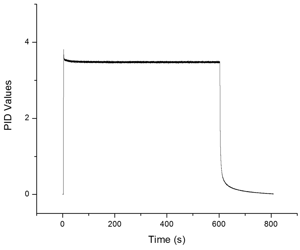
Recorded PID values from a single 10 minute-long odor stimulation session.

To explore whether there was any significant variation between individual odor pulses, seen over the whole odor stimulus, we calculated an average of all odor pulses for both 1 and 3 second-long odor pulses using a total flow of 3L/m. Figure 7A depicts a subsample of the raw PID values for four consecutive odor pulses. The raw PID responses were then realigned by trigger-onset and averaged. As seen in Figures 7B and 7C, concentration values are stable over the whole presentation for both 1 and a 3 second-long odor pulses using identical paradigms. In contrast to the many olfactometers that use a continuous flow system (described above in detail), in which air flows constantly over the odor source and is evacuated by vacuum until delivery, this system samples from the odor source and odorizes the airstream only when necessary. This style of delivery ensures that the odor source is not severely depleted over the course of a stimulation session.

Figure 7.

(A) Raw PID values for four consecutive presentations and the corresponding TTL pulse triggering odor delivery. (B) Averaged PID signal over 1s odor stimulus. (C) Averaged PID signal over 3s odor stimulus. Shaded area in graphs represents standard deviation.

3.3 Chemosensory ERP results

Clear ERP responses to the chemosensory stimuli were obtained in all the analyzed midline electrodes (Figure 8A). Amplitudes for the N1 and P2 components at the Cz electrode were −4.33 µV and 4.10µV, respectively. Moreover, detected latencies of the N1 and P2 components at the Cz electrode were 387ms and 475ms, respectively. If we add the stimulus onset time of 230ms to the latencies, a mechanical delay that we have factored out but that is included in most chemosensory ERPs in the literature, we obtain values that correspond closely with previously published data (Lorig et al., 1999; Lundstrom & Hummel, 2006; Morgan, Geisler, Covington, Polich, & Murphy, 1999). As can be seen in Figure 8B, the ERP response was not mediated by eye blink artifacts, and there was no corresponding signal for the time-locked analyses of the clean air stimuli. The latter result indicates an absence of a perceived shift in airflow when changing odor channels.

Figure 8.

(A) ERP responses to the chemosensory stimuli from midline electrodes, averaged over 38 stimuli, as well as recorded eye blinks. B) ERP to the odorless control averaged over 36 stimuli. C) ERP response for chemosensory stimuli from the Cz electrode with N1 and P2 deflections marked. In all graphs, vertical dotted blue line indicates stimulus onset. Stimuli were presented via an intranasal nose piece at a flow rate of 1.5l/m per nostril. Please note the difference in scaling between upper and lower graphs.

Taken together, these results demonstrate that the olfactometer can be used to acquire chemosensory ERPs. The temporal resolution, temporal precision, and stimulus stability of this olfactometer exceed the requirements for ERP experiments and other such experiments that demand careful timing parameters.

3.4 SCR results

In the skin conductance response (SCR) experiment, both odorants were rated as fairly intense. Subjects rated menthol as more intense (5.66; SEM ± .31; t(22) = 4.5, p < .01) than PEA (4.86; SEM ± .29). This demonstrates that the olfactometer can deliver a clear odor percept, regardless of odorant-volatility. Moreover, both odorants elicited clear evoked SCR (Figure 9). Average, baseline-corrected SCR amplitudes 10s post-stimulus were 0.14µS (SEM ± .026) for menthol and 0.10µS (SEM ± .021) for PEA.

Figure 9.

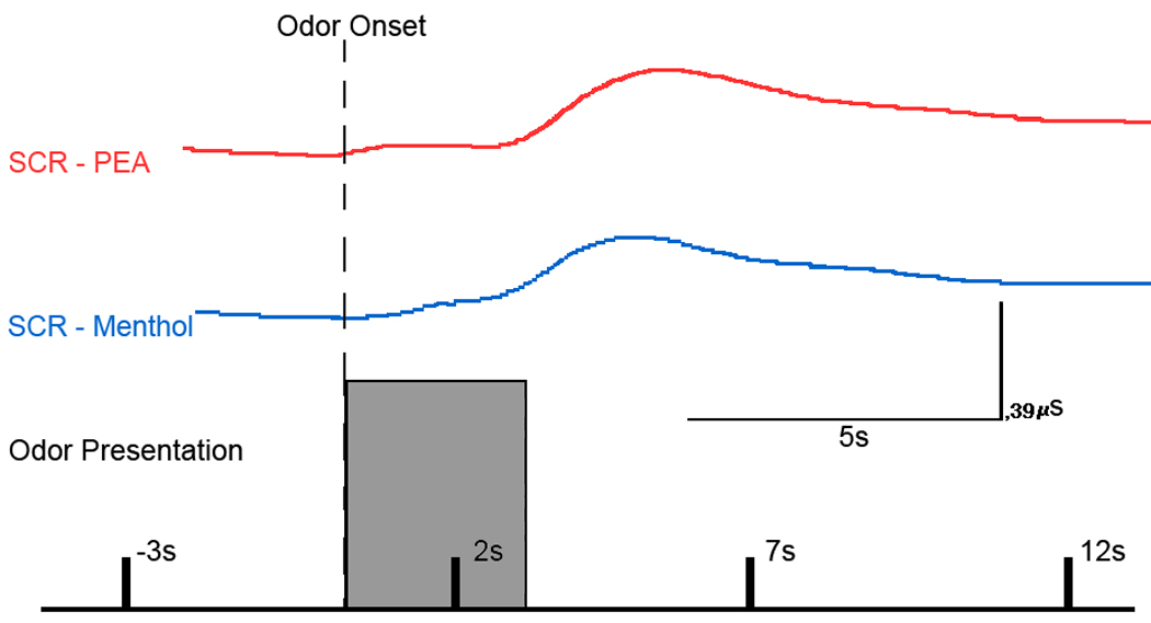
Sniff-adjusted SCR responses to the 3s odor presentation (grey block) for the two odorants. Responses were selected randomly but originate from the same subject. SCR for PEA is depicted in red, whereas SCR for menthol is depicted in blue. The dotted vertical line marks odor onset.

To assess changes in perceived stimulus intensity over time, we examined whether sensory ratings obtained during the first half of the recordings were significantly different from those obtained during the second half. Given the large time gap between odor presentations, sensory adaptation should be nominal, and any differences in sensory ratings might indicate a change in odor percept over the course of the experiment due to potential variation in odor delivery and – in turn – a design flaw. However, there was no significant difference between the first and second half of the stimulation with respect to intensity and irritation ratings, as judged with Student’s t-tests (all t < 1.12, all p > .27). Moreover, there was no significant correlation between time and ratings, as judged by Pearson correlation analyses (all r < .14, all p > .33). In other words, just as the GC/MS and the PID recordings indicated stable odor concentration over time, these data indicate that the perceived odor signal is stable throughout a behavioral experiment and that clear psychophysiological responses can be recorded.

3.5 Tonic pain ratings

As can be seen in Figure 10, participants rated the pain experience as negligent even after a 40 minute-long exposure session. The average pain rating (in rating units) for the first 10 minutes was 1.69, and the average for the last 10 minutes was 1.95. The minor increase of 0.26% pain rating units demonstrates that there was no increase over time in pain ratings. Figure 10 also demonstrates that in a comparison of pain ratings generated by airflow from this olfactometer and from the Burghart OM6b, there is no visual difference in levels perceived pain generated by room temperature air and heated, humidified air. Together with the previous finding of Lotsch and colleagues (1998), who demonstrated that a 5L/m airflow did not produce significant pain experiences, these data clearly demonstrate that a flow of 3L/m from this olfactometer does not induce any pain sensations, even in sessions as long as 40 minutes.

3.6 Potential design alterations

It is desirable in some experimental designs to use high to very high airflow for stimulus presentation. However, using airflow above 5 L/m is known to produce an increase in irritation and pain caused by desiccation of the nasal mucosa (Lotsch et al., 1998). When a higher airflow is needed, the solution is to either add heat and humidity to the airflow or to deliver the stimulus using a mask. Because this present design does not include heating and humidification of the air, we recommend a maximum flow rate of 3 L/m (1.5 L/m per nostril) with this olfactometer. While the addition of heat and humidity is relatively easy from a mechanical perspective, the total cost would rise. A simple mechanical solution would be adding a water heater, a water pump, a thermostat, and an outer layer of insulating tubing. The pump would circulate warm water within this second layer of larger diameter tubing, which would surround the smaller diameter tubing containing odorized and control air. Warmed water would be pumped from the olfactometer to the subject’s nosepiece and back, thereby providing heat to the air inside. In addition, the continuous flow would be passing through the warm water, picking up humidity and in turn humidifying the air delivered to the subject at the nosepiece. A similar simple system is described by Johnson and Sobel (2007), and this general design is currently used in the Burghart olfactometers. However, it should be noted that the addition of heating and humidification leads to a significant increase in required maintenance. The level of heat and humidity needed to mimic the intranasal environment is the perfect bacterial incubator. Therefore, distilled water is needed, and regular cleaning is required to avoid a dangerous buildup of bacteria.

If air were supplied via a compressor rather than via a central air system, the compressor would run continuously in order to provide a constant stream of air. Therefore, to reduce compressor activity, we have added a compression tank to another olfactometer constructed in our lab. This has an added benefit in that the compressor only runs intermittently when the pressure in the tank is near depletion and, depending on the size of the tank and air-outtake, the compressor might only run a few times per experiment. However, in addition to the compressor and the pressure tank, a pressure switch is needed to control the onset and offset pressure of the compressor, and a pressure regulator is needed to bring the pressure back down to breathable airflow levels.

3.7 Conclusion

In conclusion, we hope that the description of this olfactometer is detailed enough to function as a manual for those interested in building a similar device. We would like to stress that we are not claiming to have revolutionionized the field of olfactometry. Our sole claim is that the olfactometer described within this article provides interested olfactory researchers with the means to present temporally-precise odor stimuli originating from a large variety of sources in an automated fashion at a comparably low price using mainly “off-the-shelf”parts.

References

- Benignus VA, Prah JD. A computer-controlled vapor-dilution olfactometer. Behavior Research Methods & Instrumentation. 1980;12(5):535–540. [Google Scholar]
- Cain WS. Odor Magnitude - Coarse vs Fine-Grain. Perception & Psychophysics. 1977;22(6):545–549. [Google Scholar]
- deWijk RA, Vaessen W, Heidema J, Koster EP. An injection olfactometer for humans and a new method for the measurement of the shape of the olfactory pulse. Behavior Research Methods Instruments & Computers. 1996;28(3):383–391. [Google Scholar]
- Etcheto M. A constant flow-rate olfactometer with seven calibrated concentrations. Chemical Senses. 1980;5(1):1–9. [Google Scholar]
- Johnson BN, Sobel N. Methods for building an olfactometer with known concentration outcomes. J Neurosci Methods. 2007;160(2):231–245. doi: 10.1016/j.jneumeth.2006.09.008. [DOI] [PubMed] [Google Scholar]
- Kobal G. Pain-related electrical potentials of the human nasal mucosa elicited by chemical stimulation. Pain. 1985;22(2):151–163. doi: 10.1016/0304-3959(85)90175-7. [DOI] [PubMed] [Google Scholar]
- Lorig TS, Elmes DG, Zald DH, Pardo JV. A computer-controlled olfactometer for fMRI and electrophysiological studies of olfaction. Behav Res Methods Instrum Comput. 1999;31(2):370–375. doi: 10.3758/bf03207734. [DOI] [PubMed] [Google Scholar]
- Lotsch J, Ahne G, Kunder J, Kobal G, Hummel T. Factors affecting pain intensity in a pain model based upon tonic intranasal stimulation in humans. Inflamm Res. 1998;47(11):446–450. doi: 10.1007/s000110050359. [DOI] [PubMed] [Google Scholar]
- Lowen SB, Lukas SE. A low-cost, MR-compatible olfactometer. Behavior Research Methods. 2006;38(2):307–313. doi: 10.3758/bf03192782. [DOI] [PMC free article] [PubMed] [Google Scholar]
- Lundstrom JN, Hummel T. Sex-specific hemispheric differences in cortical activation to a bimodal odor. Behavioural Brain Research. 2006;166(2):197–203. doi: 10.1016/j.bbr.2005.07.015. [DOI] [PubMed] [Google Scholar]
- Lundstrom JN, Seven S, Olsson MJ, Schaal B, Hummel T. Olfactory event-related potentials reflect individual differences in odor valence perception. Chem Senses. 2006;31(8):705–711. doi: 10.1093/chemse/bjl012. [DOI] [PubMed] [Google Scholar]
- Morgan CD, Geisler MW, Covington JW, Polich J, Murphy C. Olfactory P3 in young and older adults. Psychophysiology. 1999;36(3):281–287. doi: 10.1017/s0048577299980265. [DOI] [PubMed] [Google Scholar]
- Morton TH, Castro MP, Eichenbaum H. A computer-controlled olfactometer for behavioral assays of the sense of smell. Abstracts of Papers of the American Chemical Society. 1982;183:17–18. [Google Scholar]
- Owen CM, Patterson J, Simpson DG. Development of a continuous respiration olfactometer for odorant delivery synchronous with natural respiration during recordings of brain electrical activity. Ieee Transactions on Biomedical Engineering. 2002;49(8):852–858. doi: 10.1109/TBME.2002.800765. [DOI] [PubMed] [Google Scholar]
- Saito S, Iida T, Sakaguchi H, Kodama H. The pleasantness of odorants measured with the pressure controlled olfactometer. Chemical Senses. 1984;9(1):82–83. [Google Scholar]
- Slotnick BM, Nigrosh BJ. Olfactory stimulus-control evaluated in a small animal olfactometer. Perceptual and Motor Skills. 1974;39(1):583–597. doi: 10.2466/pms.1974.39.1.583. [DOI] [PubMed] [Google Scholar]
- Vigouroux M, Viret P, Duchamp A. A wide concentration range olfactometer for delivery of short reproducible odor pulses. Journal of Neuroscience Methods. 1988;24(1):57–63. doi: 10.1016/0165-0270(88)90033-7. [DOI] [PubMed] [Google Scholar]
Associated Data
This section collects any data citations, data availability statements, or supplementary materials included in this article.